From real data to remaining useful life estimation : an approach combining neuro-fuzzy predictions and evidential Markovian classifications.

(1)

HAL Id: hal-00494988

https://hal.archives-ouvertes.fr/hal-00494988

Submitted on 24 Jun 2010

HAL is a multi-disciplinary open access

archive for the deposit and dissemination of sci-entific research documents, whether they are pub-lished or not. The documents may come from teaching and research institutions in France or abroad, or from public or private research centers.

L’archive ouverte pluridisciplinaire HAL, est destinée au dépôt et à la diffusion de documents scientifiques de niveau recherche, publiés ou non, émanant des établissements d’enseignement et de recherche français ou étrangers, des laboratoires publics ou privés.

approach combining neuro-fuzzy predictions and

evidential Markovian classifications.

Rafael Gouriveau, Emmanuel Ramasso

To cite this version:

Rafael Gouriveau, Emmanuel Ramasso. From real data to remaining useful life estimation : an ap-proach combining neuro-fuzzy predictions and evidential Markovian classifications.. 38th ESReDA Seminar Advanced Maintenance Modelling., May 2010, Pecs, Hungary. 13 p. �hal-00494988�

(2)

From real data to Remaining Useful Life estimation: an

approach combining neuro-fuzzy predictions and evidential

Markovian classifications

Rafael GOURIVEAU and Emmanuel RAMASSO

FEMTO-ST Institute, UMR CNRS 6174 - UFC / ENSMM / UTBM Automatic Control and Micro-Mechatronic Systems Department 24, rue Alain Savary, 25000 Besançon, France

Abstract

This paper deals with the proposition of a prognostic approach that enables to face up to the problem of lack of information and missing prior knowledge. Developments rely on the assumption that real data can be gathered from the system (online). The approach consists in three phases. An information theory-based criterion is first used to isolate the most useful observations with regards to the functioning modes of the system (feature selection step). An evolving neuro-fuzzy system is then used for on-line prediction of observations at any horizons (prediction step). The predicted observations are classified into the possible functioning modes using an evidential Markovian classifier based on Dempster-Shafer theory (classification step). The whole is illustrated on a problem concerning the prediction of an engine health. The approach appears to be very efficient since it enables to early but accurately estimate the failure instant, even with few learning data.

Keywords: Prognostic, Choquet Integral, Neuro-Fuzzy Systems, Evidential Theory.

1. Introduction

Prognostic is now recognized as a key process in maintenance strategies as the estimation of the remaining useful life (RUL) of an equipment allows avoiding critical damages and spending. Industrial and academics show a growing interest in this thematic, and various prognostics approaches have now been developed. They used to be classified into three categories: model-based, data-driven, and experience-based approaches [1, 2, 3]. Assuming that it can be very difficult even impossible to provide a model of the system under study, and that it is prohibitively long to store experiences, data-driven approaches are been increasingly applied to prognostics (mainly techniques from artificial intelligence AI). However, these approaches are highly-dependent on the quantity and quality of operational data that can be gathered from the system. Thus, the purpose of this paper is to propose a method to face up this problem of lack of information and missing prior knowledge in prognostics application. The method consists in three phases. An information theory-based criterion is first used to isolate the most useful observations with regards to the functioning modes of the system (feature selection step). An evolving neuro-fuzzy

(3)

system is then used for on-line multi-step ahead prediction of observations (prediction step). The predicted observations are classified into the functioning modes using an evidential markovian classifier based on Dempster-Shafer theory (classification step). The paper is organized in three main parts. The global prognostics approach is first presented. Then, the main theoretical backgrounds of each one of the three steps are given. The whole proposition is finally illustrated in a real-world prognostics problem concerning the prediction of an engine health.

2. A data-driven prognostics approach

2.1 The approach as a specific case of condition-based maintenance

According to ISO 13381-1:2004 standard, prognostics is the "estimation of time to failure and risk for one or more existing and future failure modes" [4]. It is thereby a process whose objective is to predict the remaining useful life (RUL) before a failure occurs. However, prognostic can not be seen as a single maintenance task since the whole aspects of failure analysis and prediction must be seen as a set of activities that all must be performed. This aspect is highlighted within CBM concept (Condition-Based Maintenance). Usually, a CBM system is decomposed into seven layers, one of them being that of "prognostics" [5]. The main purpose of each layer is the following:

1. Sensor module. It provides the system with digitized sensor or transducer data. 2. Processing module. It performs signal transformations and feature extractions. 3. Condition monitoring module. It compares on-line data with expected values. 4. Health assessment module. It determines if the system has degraded.

5. Prognostics module. It predicts the future condition of the monitored system. 6. Decision support module. It provides recommended actions to fulfil the mission. 7. Presentation module. It can be built into a regular machine interface.

In this paper, only layers from 2 to 5 are considered.

2.2 Proposition of a data-driven approach

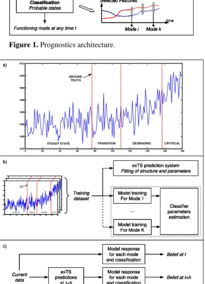
Consider a monitored system that can switch within various functioning modes. The proposed approach enables to go from multidimensional data through the remaining useful life of the system. The procedure consists in three phases (Figure 1). Data are first processed (feature extraction, selection and cleaning). It enables to feed a prediction engine which forecasts observations in time. These predictions are then analyzed by a classifier which provides the most probable state of the system. The RUL is finally deduced thanks to the estimated time to reach the failure mode. The processing, prediction and classification steps are supported by three different tools that are respectively based on information theory, evolving neuro-fuzzy systems and Dempster-Shafer theory. This is more widely explained in section 3.

Data have to be segmented into functioning modes. In Figure 2a for example, data concern the evolution of a health performance index and are segmented into four functioning modes: "steady state", "degrading state", "transition state", and "critical state". The set comprising the data and the ground truth concerning the modes is

(4)

called the training dataset. Given this dataset, an algorithm proposed in [6] is applied in order to select the most relevant set of features for each mode. This method relies on Kullback-Leibler divergence and on Choquet Integral. The training dataset is also used by both the neuro-fuzzy predictor and the classification module (Figure 2b). The NF predictor is based on the evolving extended Takagi-Sugeno system (exTS) introduced by [7]. At classification step, "modelling algorithms" are used to provide a confidence value that reflects how likely each functioning mode is at each instant. These values are then used in an Evidential Markovian Classifier (EMC) relying on the Transferable Belief Model framework [8]. When the prediction and classification modules are trained and after observing a new data at time t, the global prognostics architecture provides a belief concerning states at instant t and t+h (Figure 2c).

Processing

Extract, select, clean

Prediction

From t+1 to t+h

Classification

Probable states Multidimensional data

Functioning mode at any time t

time Mode i Selected Features Mode k time Selected Features time Selected Features time Raw data Processing

Prediction

From t+1 to t+h

Classification

Processing

Prediction

From t+1 to t+h

Classification

time Mode i Selected Features Mode k time Selected Features time Selected Features time Raw data time Mode i Selected Features Mode k time Mode i Selected Features Mode k time Selected Features time Selected Features time Selected Features time Selected Features time Raw data time Selected Features time Raw data time Selected Features time Selected Features time Raw data time Raw data

Figure 1. Prognostics architecture.

0 20 40 60 80 100 120 140 160 180 1575 1580 1585 1590 1595 1600 1605 1610

TRANSITION DEGRADING CRTITICAL STEADY STATE GROUND TRUTH 0 20 40 60 80 100 120 140 160 180 1575 1580 1585 1590 1595 1600 1605 1610

TRANSITION DEGRADING CRTITICAL STEADY STATE

GROUND TRUTH

Training dataset

exTS prediction system

Fitting of structure and parameters

Classifier parameters estimation Model training For Mode 1 Model training For Mode K … Current data exTS predictions at t+h Belief at t Belief at t+h Model response for each mode and classification

Model response for each mode and classification a) c) 0 20 40 60 80 100 120 140 160 180 1575 1580 1585 1590 1595 1600 1605 1610

TRANSITION DEGRADING CRTITICAL

STEADY STATE GROUND TRUTH b) 0 20 40 60 80 100 120 140 160 180 1575 1580 1585 1590 1595 1600 1605 1610

Classifier parameters estimation Model training For Mode 1 Model training For Mode K … 0 20 40 60 80 100 120 140 160 180 1575 1580 1585 1590 1595 1600 1605 1610

Classifier parameters estimation Model training For Mode 1 Model training For Mode K … Current data exTS predictions at t+h Belief at t Belief at t+h Model response for each mode and classification

Model response for each mode and classification Current data exTS predictions at t+h Belief at t Belief at t+h Model response for each mode and classification

Model response for each mode and classification a) c) 0 20 40 60 80 100 120 140 160 180 1575 1580 1585 1590 1595 1600 1605 1610

TRANSITION DEGRADING CRTITICAL

STEADY STATE GROUND

TRUTH

b)

Figure 2. Procedure: a) segmentation into functioning modes, b)

(5)

3. Select, predict and classify – main theoretical backgrounds

3.1 Feature selection

The aim of this step is to identify the best set of features for each mode. The applied method was initially developed in [6].

Let adopt the following notations. A data (measured or computed at t) is denoted by

Xt = [xt,1 xt,2 … xt,F], where F is the dimension of the feature space. A dataset is the

set of all data and is denoted by X = {X1, X2, …, XT} while the set of modes is denoted

by ȍ = {M1, M2, …, XK}. Li is the set of data for which the ground truth is the

functioning mode Mi. The other data are gathered in the dataset denoted Ri and the

corresponding ground truth is denoted Zi (it represents all modes except Mi). Li and Ri

are both of dimension F. Given the mode Mi, the goal is to select the dimensions of Li

which brings the most important part of the information contained in the features. The

resulting dataset will be denoted Li' with dimension Fi' F.

The method works as follows. All possible combinations of features are considered.

Given a particular combination Y

⊆

X, two probability distributions based on the data

in Li and Zi can be estimated: these two probability distributions, denoted P(Y| Mi)

and P(Y| Zi), with Y

⊆

X, are actually defined conditionally to Mi and Zi and are both

expressed on the joint space of the considered set of features. The divergence between these distributions reflects how discriminative the current set of features for the considered mode is. The chosen divergence is the Kullback-Leibler one:

(

)

( ) ( ) log ( ) ( )

i i i i

Y

KL Y =

¦

P Y M P Y M P Y Z (1)

One set of 2F divergence measures is thus computed for each mode. Given a mode

Mi, the subset of features Li' with the highest value of KLi(Li') (and the lowest

cardinality Fi') is chosen. The subsets Li' will then be used in classification.

The method described in [6] also enables to build weights reflecting importance, redundancies and complementarities of each subset of features. Let consider one

subset Y

∈

2F in the set of divergence measures for a given mode Mi. The weight of

each feature f

∈

Y in the considered subset Y is given by:

(

)

₍

_{{ }}

₎

-- -1 ! ! ( ) - ( ) ! f A Y f n A A v A f A n

µ

⊆ =

¦

× ∪ (2)

and the interaction coefficient between two features f

∈

Y and g

∈

Y is given by:

(

)

{ }

, - , - - 2 ! ! ( , ) ( ) ( ) ( ) ( -1)! f g AÍY f g n A A I A f g A f A g A n

µ

=

¦

×ª_¬ ∪ º_¼− ∪ − ∪ + (3)

where the importance coefficient

µ

(S) of a subset S is given by the value of the

(6)

( )S KL S_i( ) KL X_i( )

µ

= (4)

Given a mode Mi, the coefficients

ν

and I represent the 2-additive Choquet Integral

parameters while coefficient

µ

represents the generalized Choquet Integral

parameters. If the interaction coefficient If,g > 0, the features f and g are said

complementary while they are said redundant when the coefficient is negative. When

all interactions are nil, coefficients

ν

represent the weights of a weighted average [6].

This method has shown to be powerful in [6]. The main disadvantage is the necessity to compute a potentially high number of divergences that grows exponentially with the dimension F (until F = 15, usual PC technologies and softwares are sufficient).

3.2 Temporal predictions

Assuming that data are defined in an multidimensional space (at any time t,

Xt = [xt,1 xt,2 … xt,F], where F is the dimension of the feature space), the aims of the

prediction module is to forecast in time the evolution of the data values:

t t,1 t,2 t,F t+h t+p,1 t+p,2 t+p,F

X = [x x … x ] → X = [x x … x ] (5) with p = [1 , h], h being the maximum horizon of prediction.

In practice, this global prediction can be performed by building a prediction system for each one of the sub-signals. According to previous works [9], recent works focus on the interest of using hybrid systems for prediction purpose. In this paper, the evolving extended Takagi Sugeno system (exTS) introduced by [7] is used.

3.2.1 First order Takagi-Sugeno systems

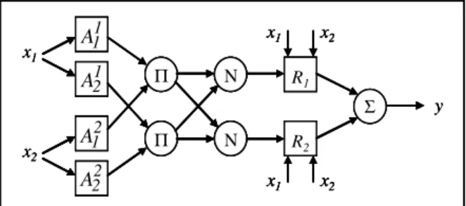
A first order TS model can be seen as a multi-model structure consisting of linear models that are not necessarily independent. It is based on the fuzzy decomposition of the input space. For each part of the state space, a fuzzy rule can be constructed to make a linear approximation of the input. The global output is a combination of the whole rules. Consider Figure 3 to explain the first order TS model. This model has two inputs variables. Two membership functions (antecedent fuzzy sets) are assigned to each one of them. The TS model is finally composed of two fuzzy rules. (That can be generalized to the case of n inputs and N rules). The rules perform a linear approximation of inputs:

1 n

i 1 i n i i i0 i1 1 in n

R : IF x is A and ... and x is A THEN y =a +a .x +...+a .x (6)

where Ri is the ith fuzzy rule, N is the number of rules, Xt = [xt,1 xt,2 … xt,F]T is the

input vector, Aij the antecedent fuzzy sets, j=[1,n], yi is the output of the ith linear

subsystem, and aiq are its parameters, q=[1,n]. Gaussian antecedent of fuzzy sets are

used to define the regions of fuzzy rules in which the local sub-models are valid:

(

)

i i* i 2

j j

j

(7)

where

σ

ij is the spread of the membership function, and xi* is the focal point (center)

of the ith rule antecedent. The firing level (

τ

i) and the normalized firing level (

λ

i) of

each rule are obtained as follows:

i i1 1 in n

Ĳ =ȝ (x )×...×ȝ (x ) , N

j=1

i i j

Ȝ = Ĳ ¦ Ĳ (8)

The model output is the weighted averaging of individual rules' contributions. With

notations

π

i = [ai0, ai1, …, ain] the vector parameter of the ith sub-model, and

xe = [1 XT]T the expanded data vector, the output is defined as:

T

N N

i i i e i

i=1 i=1

y=¦ Ȝ y =¦ Ȝ x ʌ (9)

A TS model has two types of parameters. The non-linear parameters are those of the membership functions (a Gaussian membership has two parameters: its center and its spread deviation). These kinds of parameter are referred to as premise or antecedent parameters. The second types of parameters are the linear ones that form the

consequent part of each rule (aiq). All this parameters must be tuned to fit to the

studied problem. This is the aim of the learning procedure.

Π Π Ν Ν Σ y x1 x2 R1 R2 x1 x2 x1 x2 1 1 A 1 2 A 2 2 A 2 1 A _Π Π Ν Ν Σ y x1 x2 R1 R2 x1 x2 x1 x2 1 1 A 1 2 A 2 2 A 2 1 A _Π Π Π Π Ν Ν Ν Ν Σ y x1 x2 R1 R2 R1 R2 x1 x2 x1 x2 x1 x2 x1 x2 1 1 A 1 2 A 2 2 A 2 1 A

Figure 3. A First-order TS model with 2 inputs.

3.2.2 Learning procedure of the exTS

The learning procedure of exTS is composed of two phases: (1) an unsupervised data clustering technique is used to adjust the antecedent parameters, (2) the supervised recursive least squares learning method is used to update the consequent ones. These algorithms can not be fully detailed in this paper but are well described in [7, 10]. The exTS clustering phase processes on the global input-output data space:

z = [xT ; yT]T, z

∈

Rn+m, where n+m defines the dimensionality of the input/output data space. Each one of the sub-model of exTS operates in a sub-area of z. This clustering algorithm is based on the calculus of a potential which is the capability of a data to form a cluster (antecedent of a rule). The procedure starts from scratch and, as more data are available, the model evolves by replacement or upgrade of rules. This enables the adjustment of the antecedent parameters (the non-linear ones).

Note that the main advantages of the exTS system result from the clustering phase since any assumption on the structure and parameters initialization is necessary. Indeed, an exTS is able to update the parameters without the intervention of an expert and has a flexible structure that evolves as data are gathered (new rules are formed or the existing ones are modified).

(8)

3.2.3 Using an exTS for prediction

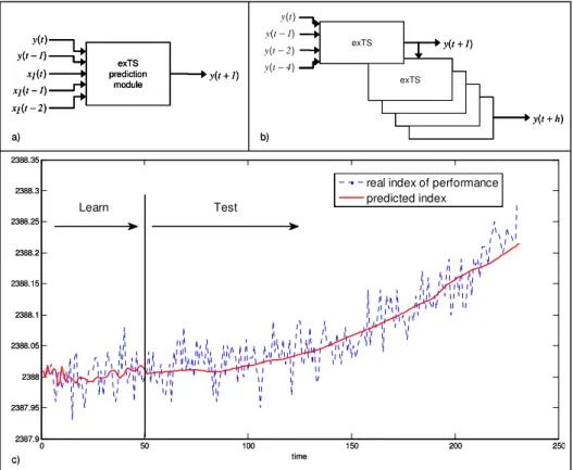
In forecasting applications, models are usually built by considering some past values of each input and output variables. Consider Figure 4a as for an example. In this figure, the NF system is composed of 2 input variables, predictions are made at one step ahead (t+1), one regressor is used for variable y and two for variable x1. In the case of a mono-variable predictor (and assuming that future is for essence unknown), previous predictions can be used as for the inputs for next predictions (Figure 4b). This type of architecture, named "cascade models" enables to perform multi-step ahead predictions (at t+h) without building various predictors (and thereby with a single learning phase).

Figure 4c shows the evolution of a performance index of an engine and the prediction that can be obtained thanks to an exTS. Note that in this figure, all predictions (from 51 to 231) where made at time t = 50.

0 50 100 150 200 250 2387.9 2387.95 2388 2388.05 2388.1 2388.15 2388.2 2388.25 2388.3 2388.35 time

real index of performance predicted index Test Learn exTS prediction module y t(+1) y t( ) y t( −1) x t1( ) x t₁(−1) x t1( −2) exTS exTS exTS exTS exTS y t(+1) y t( ) y t(−1) y t(−2) y t(−4) y t(+h) a) b) c) 0 50 100 150 200 250 2387.9 2387.95 2388 2388.05 2388.1 2388.15 2388.2 2388.25 2388.3 2388.35 time

real index of performance predicted index Test Learn exTS prediction module y t(+1) y t( ) y t( −1) x t1( ) x t₁(−1) x t1( −2) exTS prediction module y t(+1) y t( ) y t( −1) x t1( ) x t₁(−1) x t1( −2) exTS exTS exTS exTS exTS y t(+1) y t( ) y t(−1) y t(−2) y t(−4) y t(+h) exTS exTS exTS exTS exTS y t(+1) y t( ) y t(−1) y t(−2) y t(−4) y t( ) y t(−1) y t(−2) y t(−4) y t(+h) a) b) c)

Figure 4. Using an exTS for prediction: a) forecasting model with regressors,

b) cascade structure for multi-step ahead prediction, c) example of predictions result. 3.3 Classification of temporal predictions

Given observations that can be measured at t or computed by exTS at t+h, the aim of this module is to provide a reliable classification into one of the functioning modes. The proposed classification method relies on one model of data for each functioning mode. Given these models and new observations, a decision-making process is used to choose the best functioning mode. This process is temporal i.e. it embeds past and current knowledge on the functioning modes thanks to a state sequence recognition algorithm. The main idea is that the sequence of modes leads to a more reliable

(9)

conclusion concerning the real functioning mode than a decision based on modes only. Most of methods implementing this idea were based on probability theory. We propose here to exploit the framework of "Transferable Belief Model" (TBM) proposed by Ph. Smets [8]. It is based on belief functions (instead of probabilities) extending the work on Evidence Theory of Dempster and Shafer [11, 12]. On this basis, we propose to use an efficient method for state sequence recognition based on noisy observations in the TBM, that we introduced in [13].

3.3.1 Belief functions in the Transferable Belief Model

We first recall the basics on belief functions. Let ȍ = {M1, M2, … MK} be the frame of

discernment (FoD) gathering all possible and exclusive hypotheses. The number of

hypotheses is called cardinal and denoted |ȍ|. The distributions of masses, also called

Basic Belief Assigment (BBA), is defined on all possible subsets of the FoD which is

2ȍ ={{M1}, {M2}, {M1, M2}, {M3}, {M1, M2, M3}, … {ȍ}}. A subset is denoted for

example S

⊆

2ȍ or equivalently Y

∈

2ȍ. The BBA is then defined as follows:

: 2 [0,1]

m Ω a , S mΩ( )S with ( ) 1

S

mΩ S =

¦ (10)

Several functions can be computed which allow to interpret the BBA content and also to simplify combinations of BBA. The main functions are the plausibility function

(plȍ), the credibility function also called belief function (belȍ), the commonality

function (qȍ), and the weights of the canonical conjunctive decomposition (wȍ):

( 1) 1 ( ) ( ) , ( ) ( ) ( ) ( ) , ( ) ( ) C S C S C S A S A S pl S m C bel S m C q S m C w S q A Ω Ω Ω Ω ∩ ≠∅ ∅≠ ⊆ Ω Ω Ω − ⊇ ⊇ − + = ¦ = ¦ = ¦ = ∏ (11)

Mathematical backgrounds of belief functions can not be largely discussed here. Refer to [8, 14] for a deeper understanding. Let however note that the framework enables to provide decision-making processes, notably for classification problems. 3.3.2 Evidential Hidden Markov Models (EvHMM)

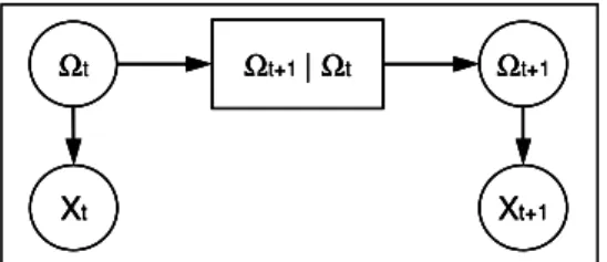
An extension of probabilistic Hidden Markov Models (HMM) to the TBM is proposed in [13]. To represent EvHMM, we use an extension of Directed Evidential Network to the temporal domain that we call Temporal DEVN (TDEVN). A TDEVN is depicted in Figure 5. The advantages of this framework are listed here after:

− it enables to represent lack of knowledge on states, e.g. at the first instant the prior on states can be vacuous,

− the estimation of the network parameters is improved by using a training set annotated by belief functions [13, 15],

− the inference of the state sequence based on noisy observations is improved by using the evidential Viterbi-like decoder proposed in [13],

− possibly non-distinct (not independent) observations can be considered using particular combinations rules [16].

− It enables to combine several types of formalisms for uncertainty management in a common framework.

(10)

Ωt+1 | Ωt Ωt Xt Ωt+1 Xt+1 Ωt+1 | Ωt Ωt Xt Ωt+1 Xt+1 Ωt+1 | Ωt Ωt+1 | Ωt Ωt Ωt Xt Xt Ωt+1 Ωt+1 Xt+1 Xt+1

Figure 5. TDEVN representing EvHMM.

Classification of sequence of observations in EvHMM

Given a set of T observations X1:T (with dimension F), it is possible to recursively

compute the likelihood of the sequence by using the forward belief function. For a

particular EvHMM

λ

, the forward variable is given by eq. (12). In order to represent

missing prior at the first instant, one can use a vacuous BBA: Ω1(Ω₁)=1

α

m . If

observations are distinct, one may use the commonalities instead of weights.

At each instant, the conflict value m_αΩt(∅) represents the amount of mass which is

allocated to subsets not in _{2 and therefore, the total amount of conflict in the whole}Ωt

sequence quantifies how unlikely are the observations given the model [13]. The

conflict value is linked to the plausibility by m (Æ)=1-pl_Įȍt _Įȍt(ȍ ). Thus, it is possible _t

to compute the sequence plausibility for a particular EvHMM

λ

like in eq. (13). and

then the best model is given by maximizing L(

λ

) over all models

λ

.

1 1 ( ) T log ( _t) t t L pl T α λ Ω = = ¦ Ω (13)

State sequence recognition in EvHMM

Given a sequence of noisy observations, one may be interested in knowing which state is the best one at a given instant. This can be made thanks to an evidential Viterbi-like decoder that allows propagating the decision at t over the states at subsequent instants [13]. An evidential Viterbi-like decoder is based on the propagation of the following metric:

1 1 1 ( ) ( ) _a [ ]( ) _b [ _t]( ) B t t t t t t w_δΩ S m_δΩ B wΩ Ω B S wΩ ℜ X S ⊆ℑ − − − ª º =_« ¦ × _»⊗ ¬ ¼ (14)

The difference with the forward variable is the computation of the sum which is now

done over subsets of ℑ_t₋₁ that is actually a subset of Ωt₋₁. The hypotheses composing

1 −

ℑt are selected at each instant. First, the set of weights

t j wδΩ, are computed: , 1 1 1 ( ) ( ) _a [ _j]( ) [ _t]( ) j b B t t t t t t w_δΩ S m_δΩ B wΩ Ω B M S wΩ ℜ X S ⊆Ω − − − ª º =_« ¦ × ∩ _»⊗ ¬ ¼ (15)

(11)

This equation is simply a forward propagation but conditioned on each mode Mj∈ȍt-1.

One obtains a set of weights for each mode. These weights are then transformed into

BBA _,t( )

j

m_δΩ S and then into pignistic probability distributions. We thus obtain a set of

|ȍt-1| pignistic distributions defined on ȍt conditionally to each mode. The best

predecessor of a mode Mi∈ is thus found and stored and the set Ωt ℑt−1 is composed

by the union of predecessors:

{ }

, 1 1 1 ( ) arg max ( ) , ( ) t i j i t t i i M t t t j t M BetP m_δ M M ψ Ω Ω Ω ψ − ∈Ω − − = ℑ = (16)

At instant t, it is possible to compute the state sequence from t0. For that, the best

mode t

M_* at t must be computed in order to use the backtracking process until t0:

{ }

* , 1 arg max ( ) t i j M t t j t M BetPΩ m_δΩ M ∈Ω₋ = , M_*t−1=

ψ

_t(M_*t) (17)

Parameter learning in EvHMM

In this paper, the training set is composed of observations for which the ground truth (real modes) is known. In this case, each mode can be modeled using an EM clustering assuming Gaussian mixtures. Given trained models, a new observation generates a set of likelihoods (one for each mode) which are then used in the Generalized Bayesian Theorem in order to compute the posterior BBA on the set of modes given observations. These posterior BBA are then used to estimate automatically the evidential transition matrix. The method consists in computing the

expected joint belief mass defined on the product space ȍt× ȍt-1 over all time

instants. This can not be fully described in this paper.

4. Experiments and results

4.1 Experimental dataset and prognostics procedure

The proposed data-driven procedure is illustrated by using the challenge dataset of diagnostic and prognostics of machine faults from the first International Conference on Prognostics and Health Management (2008) [18]. The dataset consisted of multiple multivariate time series (26 variables) with sensor noise (like in Figure 2a). Each time series was from a different engine of the same fleet and each engine started with different degrees of initial wear and manufacturing variation unknown to the user and considered normal. The engine was operating normally at the start and developed a fault at some point. The fault grew in magnitude until system failure. Given a new observation sequence, the goal was to diagnose its current and future mode by the proposed procedure in order to determine the remaining time before failure, assuming that a fault has occurred when a sequence of four modes has been

detected (steady ĺ transition ĺ degrading ĺ faulty). For tests, 40 multivariate time

(12)

From the 26 features, we first aimed at selecting only 8 of them. We first built all groups of 8 features and applied the feature selection method. For each mode, the group with the maximum value of the Kullback-Leibler divergence has been selected. Then, we applied again the feature selection process considering all combinations of features among the group of eight. Note that the group of features for each mode was generally different. Following that, one detector has been built for each mode. For that, an EM has been run on the training set using mixture of Gaussians with adaptive number of components. For the prediction step, each feature has been estimated with an exTS model for multi-step ahead prediction (a NF cascade model as explained before). Table I resumes the set of inputs variables used for that purpose. All predictions were made until time t = 50, so that, for each data test set, the prediction module provided the expected values of the considered performance index from time

t = 51 to the end of the test series. For the classification step, a four states EvHMM

has been built where the evidential transition matrix was estimated as proposed in this paper (using the training set).

Table I: Feature prediction with exTS.

Feature Inputs Feature Inputs

F 1 t, x1(t), x1(t-1), x1(t-2) F 5 t, x5(t)

F 2 t, x2(t), x2(t-1), x2(t-2) F 6 t, x6(t)

F 3 t, x3(t), x3(t-1), x3(t-2) F 7 t, x7(t), x7(t-1)

F 4 t, x4(t), x4(t-1) F 8 t, x8(t), x8(t-1)

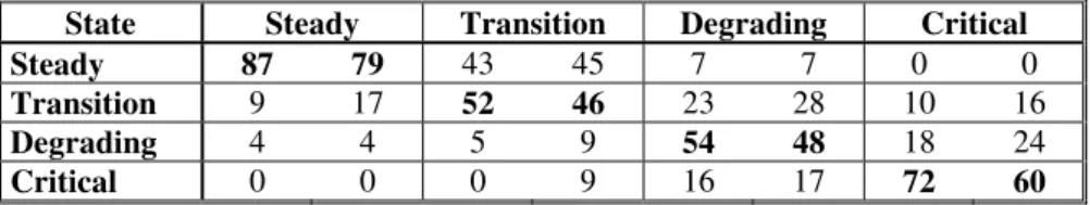
4.2 Results and discussion

Simulation results are reported in Table II (left side of boxes) that is a confusion matrix. As for an example of how to interpret it, consider the box {Transition ,

Steady}: in 9% of test for which the right classification of the functioning mode

would have been "steady state", the procedure classified it into a "transition mode". In order to extract more solid conclusions on the proposed approach, a comparison has been made with the use of probabilistic HMM for classification (Table II, right side).

Table I: Confusion matrix for state detection using: a) EvHMM (left side), b) HMM (right side). State Steady Transition Degrading Critical

Steady 87 79 43 45 7 7 0 0

Transition 9 17 52 46 23 28 10 16

Degrading 4 4 5 9 54 48 18 24

Critical 0 0 0 9 16 17 72 60

Results show good performance in detecting states with the EvHMM, in particular the critical and the steady states. The main problems appear in detecting both the transition and degrading states: the former is of short duration and thus difficult to detect while the latter is highly evolving. The overall detection is slightly more stable with the evidential version than with the probabilistic HMM (an example is given in Figure 6), in particular the detection of the "transition" and "degrading" states. This is mainly due to the Viterbi-like decoder which postpones the decision until the last instants thanks to the conditioned forward propagation. The RUL of the engine can finally be estimated as the difference in between the instant in which the engine is supposed to be in a critical state and the current time (Figure 6).

(13)

0 50 100 150 200 250 300 0 0.5 1 1.5 2 2.5 3 3.5 4 EvHMM HMM Features

Estimated Remaining Useful Life (RUL)

0 50 100 150 200 250 300 0 0.5 1 1.5 2 2.5 3 3.5 4 EvHMM HMM Features

Estimated Remaining Useful Life (RUL)

Figure 6. Example of result. Green dots: data normalized in [0,4] for

visualization. State detection: blue dashed line for HMM, red line for EvHMM.

7. Conclusion

In this paper, a data-driven approach to prognostic the system health of an equipment is proposed. The method enables to face up this problem of lack of information and missing prior knowledge in real applications, that reduces the applicability of conventional artificial techniques. The approach is based on the integration of three modules and aims at predicting the failure mode early while the system can switch between several functioning modes. The three modules are: an information theory-based feature selection process, an exTS for reliable multi-step ahead predictions and an evidence theory-based Markovian classifier for state detection. The efficiency of the proposed architecture is showed on a real data set concerning an engine health. In particular, the average horizon for predictions used in experiments is close to t+130 time units and despite this challenging condition, the overall performance of the evidential classification of states is around 70%. Comparisons with probabilistic HMM for state classification also clearly show the efficiency of the approach.

References

[1] Byington, C., Roemer, M., Kacprzynski, G. Galie, T. (2002). Prognostic enhancements to diagnostic systems for improved condition-based maintenance, In: Proc. IEEE Int. Conf. on Aerospace, vol. 6, pp. 2815-2824. [2] Vachtsevanos, G. et al. (2006). Intelligent Fault Diagnostic and Prognosis for

Engineering Systems, John Wiley & Sons.

[3] Heng, A., Zhang, S., Tan, A. and Matwew, J. (2009). Rotating machinery prognostic: State of the art, challenges and opportunities, Mechanical Systems

and Signal Processing, vol. 23, pp. 724-739.

[4] ISO (2004). Condition monitoring and diagnostics of machines, prognostics -

(14)

[5] Lebold, M. and Thurston, M. (2001) Open standards for condition-based maintenance and prognostics systems, In: Proc. of 5th Annual Maintenance and

Reliability Conference.

[6] Jullien, S., Valet, L., Mauris, G., Bolon, Ph. and Teyssier, S. (2008). An attribute fusion system based on the Choquet Integral to evaluate the quality of composite parts, IEEE Trans. on Instrum. & Measur., vol. 57, pp. 755-762. [7] Angelov, P. and Filev, D. (2004). An approach to online identification of

takagi-sugeno fuzzy models, IEEE Trans. Syst. Man Cybern. - Part B:

Cybernetics, vol. 34, pp. 484-498.

[8] Smets, Ph. and Kennes, R. (1994). The Transferable Belief Model, Artificial

intelligence, vol. 66:2, pp. 191-234.

[9] El-Koujok, M., Gouriveau, R. and Zerhouni N. (2009). Error estimation of a neuro-fuzzy predictor for prognostic purpose, In: Proc. 7th Int. Symp. on Fault

Detection, Supervision and Safety of Technical Processes, SAFE PROCESS'09.

[10] Angelov, P. and Zhou, X. (2006). Evolving fuzzy systems from data streams in real-time, In: Proc. Int. Symp. On Evolving Fuzzy Systems, pp. 26-32.

[11] Dempster, A.P. (1967). Upper and lower probabilities induced by a multivalued mapping, Annals of Mathematical Statistics, vol. 38, pp. 325-339.

[12] Shafer, G. (1976). A mathematical theory of evidence, Princeton University Press, Princeton N.J.

[13] Ramasso, E. (2009). Contribution of belief functions to Hidden Markov Models with an application to fault diagnosis, In: Proc. IEEE Int. Workshop on

Machine Learning and Signal Processing.

[14] Smets, Ph. (1993). Belief functions: the disjunctive rule of combination and the generalized Bayesian theorem, Int. Jour. of Approx. Reasoning, vol. 9, pp. 1-35. [15] Côme, E., Oukhellou, L., Denoeux, T. and Aknin, P. (2009). Learning from

partially supervised data using mixture models and belief functions, Pattern

Recognition, vol. 42, pp. 334-348.

[16] Denoeux, T. (2008). Conjunctive and Disjunctive Combination of Belief Functions Induced by Non Distinct Bodies of Evidence, Artificial Intelligence, vol. 172, pp. 234-264.

[17] Saxena, A., Goebel, K., Simon, D. and Eklund, N. (2008). Damage Propagation Modeling for Aircraft Engine Run-to-Failure Simulation, In: Proc. IEEE