HAL Id: hal-00871750
https://hal.archives-ouvertes.fr/hal-00871750
Submitted on 15 Oct 2013
HAL is a multi-disciplinary open access
archive for the deposit and dissemination of
sci-entific research documents, whether they are
pub-lished or not. The documents may come from
teaching and research institutions in France or
abroad, or from public or private research centers.
L’archive ouverte pluridisciplinaire HAL, est
destinée au dépôt et à la diffusion de documents
scientifiques de niveau recherche, publiés ou non,
émanant des établissements d’enseignement et de
recherche français ou étrangers, des laboratoires
publics ou privés.
Three Generalizations of the FOCUS Constraint
Nina Narodytska, Thierry Petit, Mohamed Siala, Toby Walsh
To cite this version:
Nina Narodytska, Thierry Petit, Mohamed Siala, Toby Walsh. Three Generalizations of the FOCUS
Constraint. 23rd International Joint Conference on Artificial Intelligence (IJCAI 2013), Aug 2013,
Beijing, China. p.630 ; ISBN 978-1-57735-633-2. �hal-00871750�
Three Generalizations of the FOCUS Constraint
Nina Narodytska
NICTA and UNSW
Sydney, Australia
[email protected]
Thierry Petit
LINA-CNRS
Mines-Nantes, INRIA
Nantes, France
[email protected]
Mohamed Siala
LAAS-CNRS
Univ de Toulouse, INSA
Toulouse, France
[email protected]
Toby Walsh
NICTA and UNSW
Sydney, Australia
[email protected]
Abstract
The FOCUSconstraint expresses the notion that so-lutions are concentrated. In practice, this constraint suffers from the rigidity of its semantics. To tackle this issue, we propose three generalizations of the FOCUSconstraint. We provide for each one a com-plete filtering algorithm as well as discussing de-compositions.
1
Introduction
Many discrete optimization problems have constraints on the objective function. Being able to represent such constraints is fundamental to deal with many real world industrial prob-lems. Constraint programming is a promising approach to express and filter such constraints. In particular, several constraints have been proposed for obtaining well-balanced solutions [Pesant and R´egin, 2005; Schaus et al., 2007; Petit and R´egin, 2011]. Recently, the FOCUSconstraint [Pe-tit, 2012] was introduced to express the opposite notion. It captures the concept of concentrating the high values in a se-quence of variables to a small number of intervals. We recall its definition. Throughout this paper, X = [x0, x1, . . . , xn−1]
is a sequence of variables and si,jis a sequence of indices of
consecutive variables in X, such that si,j = [i, i + 1, . . . , j],
0 ≤ i ≤ j < n. We let |E| be the size of a collection E. Definition 1 ([Petit, 2012]). Let ycbe a variable. Letk and
len be two integers, 1 ≤ len ≤ |X|. An instantiation of X ∪ {yc} satisfies FOCUS(X, yc, len, k ) iff there exists a set SX
ofdisjoint sequences of indices si,jsuch that three conditions
are all satisfied: (1) |SX| ≤ yc (2) ∀xl ∈ X, xl > k ⇔
∃si,j ∈ SXsuch thatl ∈ si,j(3) ∀si,j∈ SX,j − i + 1 ≤ len
FOCUS can be used in various contexts including cumu-lative scheduling problems where some excesses of capac-ity can be tolerated to obtain a solution [Petit, 2012]. In a cumulative scheduling problem, we are scheduling activi-ties, and each activity consumes a certain amount of some re-source. The total quantity of the resource available is limited by a capacity. Excesses can be represented by variables [De Clercq et al., 2011]. In practice, excesses might be toler-ated by, for example, renting a new machine to produce more resource. Suppose the rental price decreases proportionally
to its duration: it is cheaper to rent a machine during a sin-gle interval than to make several rentals. On the other hand, rental intervals have generally a maximum possible duration. FOCUS can be set to concentrate (non null) excesses in a small number of intervals, each of length at most len.
Unfortunately, the usefulness of FOCUSis hindered by the rigidity of its semantics. For example, we might be able to rent a machine from Monday to Sunday but not use it on Fri-day. It is a pity to miss such a solution with a smaller number of rental intervals because FOCUSimposes that all the vari-ables within each rental interval take a high value. Moreover, a solution with one rental interval of two days is better than a solution with a rental interval of four days. Unfortunately, FOCUSonly considers the number of disjoint sequences, and does not consider their length.
We tackle those issues here by means of three generaliza-tions of FOCUS. SPRINGYFOCUS tolerates within each se-quence in si,j ∈ SX some values v ≤ k . To keep the
se-mantics of grouping high values, their number is limited in each si,jby an integer argument. WEIGHTEDFOCUSadds a
variable to count the length of sequences, equal to the num-ber of variables taking a value v > k . The most generic
one, WEIGHTEDSPRINGYFOCUS, combines the semantics
of SPRINGYFOCUSand WEIGHTEDFOCUS. Propagation of constraints like these complementary to an objective func-tion is well-known to be important [Petit and Poder, 2008; Schaus et al., 2009]. We present and experiment with filtering algorithms and decompositions therefore for each constraint.
2
Springy FOCUS
In Definition 1, each sequence in SXcontains exclusively
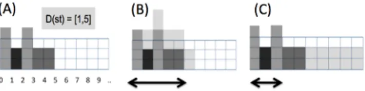
val-ues v > k. In many practical cases, this property is too strong. Consider one simple instance of the problem in the introduc-tion, in Figure 1, where one variable xi ∈ X is defined per
point in time i (e.g., one day), to represent excesses of capac-ity. Inintialy, 4 activities are fixed and one activity a remains to be scheduled (drawing A), of duration 5 and that can start from day 1 to day 5. If FOCUS(X, yc = 1, 5, 0) is imposed
then a must start at day 1 (solution B). We have one 5 day rental interval. Assume now that the new machine may not be used every day. Solution (C) gives one rental of 3 days instead of 5. Furthermore, if len = 4 the problem will have no solution using FOCUS, while this latter solution still ex-ists in practice. This is paradoxical, as relaxing the condition
Figure 1: (A) Problem with 4 fixed activities and one activity of length 5 that can start from time 1 to 5. (B) Solution satisfying FOCUS(X, [1, 1], 5, 0), with a new machine rented for 5 days. (C) Practical solution violating FOCUS(X, [1, 1], 5, 0), with a new ma-chine rented for 3 days but not used on the second day.
that sequences in the set SXof Definition 1 take only values
v > k deteriorates the concentration power of the constraint. Therefore, we propose a soft relaxation of FOCUS, where at mosth values less than k are tolerated within each sequence in SX.
Definition 2. Let yc be a variable and k , len, h be three
integers,1 ≤ len ≤ |X|, 0 ≤ h < len −1. An instantiation of X ∪ {yc} satisfies SPRINGYFOCUS(X, yc, len, h, k ) iff there
exists a setSXof disjoint sequences of indices si,jsuch that
four conditions are all satisfied:(1) |SX| ≤ yc(2) ∀xl∈ X,
xl > k ⇒ ∃si,j ∈ SX such thatl ∈ si,j (3) ∀si,j ∈ SX,
j − i + 1 ≤ len, xi > k and xj > k. (4) ∀si,j ∈ SX,
|{l ∈ si,j,xl≤ k }| ≤ h
Bounds consistency (BC) on SPRINGYFOCUS is equiva-lent to domain consistency: any solution can be turned into a solution that only uses the lower bound min(xl) or the
up-per bound max(xl) of the domain D(xl) of each xl ∈ X
(this observation was made for FOCUS[Petit, 2012]). Thus, we propose a BC algorithm. The first step is to traverse X from x0to xn−1, to compute the minimum possible number
of disjoint sequences in SX (a lower bound for yc), the
fo-cus cardinality, denoted fc(X). We use the same notation for subsequences of X. fc(X) depends on k , len and h.
Definition 3. Given xl ∈ X, we consider three quantities.
(1)p(xl, v≤) is the focus cardinality of [x0, x1, . . . , xl],
as-suming xl ≤ k , and ∀si,j ∈ S[x0,x1,...,xl], j 6= l. (2) pS(xl, v≤) is the focus cardinality of [x0, x1, . . . , xl],
assum-ingxl ≤ k and ∃i, si,l ∈ S[x0,x1,...,xl]. (3)p(xl, v>) is the focus cardinality of[x0, x1, . . . , xl] assuming xl> k .
Any quantity is equal ton + 1 if the domain D(xl) of xl
makes not possible the considered assumption.
Property 1. pS(x0, v≤) = pS(xn−1, v≤) = n + 1, and
fc(X) = min(p(xn−1, v≤), p(xn−1, v>)).
Proof. By construction from Definitions 2 and 3.
To compute the quantities of Definition 3 for xl∈X we use
plen(xl), the minimum length of a sequence in S[x0,x1,...,xl] containing xlamong instantiations of [x0, x1, . . . , xl] where
the number of sequences is fc([x0, x1, . . . , xl]). plen(xl)=0
if ∀si,j∈ S[x0,x1,...,xl], j 6= l. card (xl) is the minimum num-ber of values v ≤ k in the current sequence in S[x0,x1,...,xl], equal to 0 if ∀si,j ∈ S[x0,x1,...,xl], j 6= l. card (xl) assumes that xl > k. It has to be decreased it by one if xl ≤ k. For
sake of space, the proofs of the next four lemmas are given in a technical report [Narodytska et al., 2013].
Algorithm 1:MINCARDS(X, len, k , h): Integer matrix
1 pre := new Integer[|X|][4][] ;
2 for l ∈ 0..n − 1 do
3 pre[l][0] := new Integer[2];
4 for j ∈ 1..3 do pre[l][j] := new Integer[1];
5 Initialization Lemma 1,;
6 for l ∈ 1..n − 1 do Lemmas 2, 3, 4 and Propositions 1 and 2.;
7 return pre;
Lemma 1 (initialization). p(x0, v≤) = 0 if min(x0) ≤ k,
and n + 1 otherwise; pS(x0, v≤) = n + 1; p(x0, v>) =
1 if max(x0) > k and n + 1 otherwise; plen(x0) = 1 if
max(x0) > k and 0 otherwise; card (x0) = 0.
Lemma 2 (p(xl, v≤)). If min(xl) ≤ k then p(xl, v≤) =
min(p(xl−1, v≤), p(xl−1, v>)), else p(xl, v≤) = n + 1.
Lemma 3 (pS(xl, v≤)). If min(xi)>k, pS(xi, v≤)=n + 1.
Otherwise, ifplen(xi−1) ∈ {0, len − 1, len} ∨ card (xi−1)
= h then pS(xi, v≤) = n + 1, else pS(xi, v≤) =
min(pS(xi−1, v≤), p(xi−1, v>)).
Lemma 4 (p(xl, v>)). If max(xl) ≤ k then p(xl, v>)=n+1.
Otherwise, If plen(xl−1) ∈ {0, len}, p(xl, v>) =
min(p(xl−1, v>) + 1, p(xl−1, v≤) + 1), else p(xl, v>)
= min(p(xl−1, v>), pS(xl−1, v≤), p(xl−1, v≤) + 1).
Proposition 1 (plen(xl)). (by construction) If min
(pS(xl−1, v≤),p(xl−1, v>))<p(xl−1,v≤)+1∧plen(xl−1)<
len then plen(xl) = plen(xl−1) + 1. Otherwise, if
p(xl, v>)) < n + 1 then plen(xl) = 1, else plen(xl) = 0.
Proposition 2 (card (xl)). (by construction) If plen(xl) = 1
thencard (xl) = 0. Otherwise, if p(xl, v>) = n + 1 then
card (xl) = card (xl−1) + 1, else card (xl) = card (xl−1).
Algorithm 1 implements the lemmas with pre[l][0][0] = p(xl, v≤), pre[l][0][1] = pS(xl, v≤), pre[l][1] = p(xl, v>),
pre[l][2] = plen(xl), pre[l][3] = card (xl).
The principle of Algorithm 2 is the following. First, lb = f c(X) is computed with xn−1. We execute Algorithm 1 from
x0 to xn−1 and conversely (arrays pre and suf ). We thus
have for each quantity two values for each variable xl. To
ag-gregate them, we implement regret mechanisms directly de-rived from Propositions 2 and 1, according to the parameters
len and h. Line 4 is optional but it avoids some work
when the variable yc is fixed, thanks to the same property
as FOCUS (see [Petit, 2012]). Algorithm 2 performs a con-stant number of traversals of the set X. Its time complexity is O(n), which is optimal.
3
Weighted FOCUS
We present WEIGHTEDFOCUS, that extends FOCUS with a variable zclimiting the the sum of lengths of all the sequences
in SX, i.e., the number of variables covered by a sequence in
SX. It distinguishes between solutions that are equivalent
with respect to the number of sequences in SX but not with
respect to their length, as Figure 2 shows.
Definition 4. Let yc and zc be two integer variables
Algorithm 2:FILTERING(X, yc, len, k , h): Set of variables
1 pre := MINCARDS(X, len, k, h) ;
2 Integer lb := min(pre[n − 1][0][0], pre[n − 1][1]);
3 if min(yc) < lb then D(yc) := D(yc) \ [min(yc), lb[;
4 if min(yc) = max(yc) then
5 suf := MINCARDS([xn−1, xn−2, . . . , x0], len, k, h) ;
6 for l ∈ 0..n − 1 do
7 if pre[l][0][0] + suf [n − 1 − l][0][0] > max(yc) then
8 Integer regret := 0; Integer add := 0;
9 if pre[l][1] ≤ pre[l][0][1] then add := add + 1;
10 if suf [n − 1 − l][1] ≤ suf [n − 1 − l][0][1] then add:=add+1;
11 if pre[l][2] + suf [n − 1 − l][2] − 1 ≤ len ∧
pre[l][3] + suf [n − 1 − l][3] + add − 1 ≤ h then regret := 1;
12 if
pre[l][0][1] + suf [n − 1 − l][0][1] − regret > max(yc)
then D(xi) := D(xi)\ [min(xi), k];
13 Integer regret := 0;
14 if pre[l][2] + suf [n − 1 − l][2] − 1 ≤ len ∧
pre[l][3] + suf [n − 1 − l][3] − 1 ≤ h then regret := 1;
15 if pre[l][1] + suf [n − 1 − l][1] − regret > max(yc) then
16 D(xi) := D(xi)\ ]k, max(xi)];
17 return X ∪ {yc};
|X|. An instantiation of X ∪ {yc} ∪ {zc} satisfies
WEIGHTEDFOCUS(X, yc, len, k , zc) iff there exists a setSX
ofdisjoint sequences of indices si,jsuch that four conditions
are all satisfied: (1) |SX| ≤ yc (2) ∀xl ∈ X, xl > k ⇔
∃si,j ∈ SXsuch thatl ∈ si,j(3) ∀si,j∈ SX,j − i + 1 ≤ len
(4)P
si,j∈SX|si,j| ≤ zc.
Definition 5 ([Petit, 2012]). Given an integer k , a variable xl ∈ X is: Penalizing, (Pk), iff min(xl) > k. Neutral,
(Nk), iff max(xl) ≤ k. Undetermined, (Uk), otherwise. We
sayxl∈ Pkiffxlis labeledPk, and similarly forUkandNk.
Figure 2: (A) Problem with 4 fixed activities and one activity of length 5 that can start from time 3 to 5. We assume D(yc) = {2},
len = 3 and k = 0. (B) Solution satisfying WEIGHTEDFOCUSwith zc= 4. (C) Solution satisfying WEIGHTEDFOCUSwith zc= 2.
Dynamic Programming (DP) Principle Given a partial
in-stantiation IX of X and a set of sequences SX that
cov-ers all penalizing variables in IX, we consider two terms:
the number of variables in Pk and the number of
undeter-minedvariables, in Uk, covered by SX. We want to find a
set SX that minimizes the second term. Given a sequence
of variables si,j, the cost cst(si,j) is defined as cst(si,j) =
{p|xp ∈ Uk, xp ∈ si,j}. We denote cost of SX, cst(SX),
the sum cst(SX) = Psi,j∈SXcst(si,j). Given IX we con-sider |Pk| = |{xi ∈ Pk}|. We have: Psi,j∈S|si,j| = P
si,j∈Scst(si,j) + |Pk|.
We start with explaining the main difficulty in building a propagator for WEIGHTEDFOCUS. The constraint has two
optimization variables in its scope and we might not have a solution that optimizes both variables simultaneously. Example 1. Consider the set X = [x0, x1, . . . , x5]
with domains [1, {0, 1}, 1, 1, {0, 1}, 1] and
WEIGHTEDFOCUS(X, [2, 3], 3, 0, [0, 6]), solution SX = {s0,2, s3,5}, zc = 6, minimizes yc = 2, while
solutionSX= {s0,1, s2,3, s5,5}, yc = 3, minimizes zc= 4.
Example 1 suggests that we need to fix one of the two opti-mization variables and only optimize the other one. Our algo-rithm is based on a dynamic program [Dasgupta et al., 2006]. For each prefix of variables [x0, x1, . . . , xj] and given a cost
value c, it computes a cover of focus cardinality, denoted Sc,j, which covers all penalized variables in [x0, x1, . . . , xj]
and has cost exactly c. If Sc,j does not exist we assume that
Sc,j= ∞. Sc,jis not unique as Example 2 demonstrates.
Example 2. Consider X = [x0, x1, . . . , x7] and
WEIGHTEDFOCUS(X, [2, 2], 5, 0, [7, 7]), with D(xi) = {1},
i ∈ I, I = {0, 2, 3, 5, 7} and D(xi) = {0, 1},
i ∈ {0, 1, . . . 7} \ I. Consider the subsequence of
variables[x0, . . . , x5] and S1,5. There are several sets of
minimum cardinality that cover all penalized variables in the prefix[x0, . . . , x5] and has cost 2, e.g. S1,51 = {s0,2, s3,5}
orS2
1,5 = {s0,4, s5,5}. Assume we sort sequences by their
starting points in each set. We note that the second set is better if we want to extend the last sequence in this set as the length of the last sequences5,5 is shorter compared to the
length of the last sequence inS1
1,5, which iss3,5.
Example 2 suggests that we need to put additional condi-tions on Sc,jto take into account that some sets are better than
others. We can safely assume that none of the sequences in Sc,jstarts at undetermined variables as we can always set it
to zero. Hence, we introduce a notion of an ordering between sets Sc,jand define conditions that this set has to satisfy.
Ordering of sequences in Sc,j. We introduce an order
over sequences in Sc,j. Given a set of sequences in Sc,j we
sort them by their starting points. We denote last(Sc,j) the
last sequence in Sc,j in this order. If xj ∈ last(Sc,j) then
|last(Sc,j)| is, naturally, the length of last(Sc,j), otherwise
|last(Sc,j)| = ∞.
Ordering of setsSc,j,c ∈ [0, max(zc)], j ∈ {0, 1, . . . , n −
1}. We define a comparison operation between two sets Sc,j
and Sc0,j0. Sc,j ≤ Sc0,j0 iff |Sc,j| < |Sc0,j0| or |Sc,j| = |Sc0,j0| and last(Sc,j) ≤ last(Sc0,j0). Note that we do not take account of cost in the comparison as the current defini-tion is sufficient for us. Using this operadefini-tion, we can compare all sets Sc,jand Sc,j0 of the same cost for a prefix [x0, . . . , xj].
We say that Sc,jis optimal iff satisfies the following 4
condi-tions.
Proposition 3 (Conditions on Sc,j).
1. Sc,jcovers allPkvariables in[x0, x1, . . . , xj],
2. cst(Sc,j) = c,
3. ∀sh,g∈ Sc,j, xh∈ U/ k,
4. Sc,jis the first set in the order among all sets that satisfy
conditions 1–3.
As can be seen from definitions above, given a subse-quence of variables x0, . . . , xj, Sc,j is not unique and might
fc-1,j-1 xj-1 fc,j-1 xjin Pk fc,j xj-1 xjin Uk fc,j es fc-1,j-1 fc,j-1 xj-1 xjin Nk fc,j fc,j-1 fc-1,j-1
es - extend or start new e - extend i - interrupt (a) (b) (c) i es i e
Figure 3: Representation of one step of Algorithm 3. not exist. However, if |Sc,j| = |Sc0,j0|, c = c0 and j = j0, then last(Sc,j) = last(Sc0,j0).
Example 3. Consider WEIGHTEDFOCUS from Example 2.
Consider the subsequence[x0, x1]. S0,1 = {s0,0}, S1,1 =
{s0,1}. Note that S2,1 does not exist. Consider the
sub-sequence [x0, . . . , x5]. We have S0,5 = {s0,0, s2,3, s5,5},
S1,5 = {s0,4, s5,5} and S2,5 = {s0,3, s5,5}. By definition,
last(S0,5) = s5,5,last(S1,5) = s5,5 andlast(S2,5) = s5,5.
Consider the set S1,5. Note that there exists another set
S0
1,5 = {s0,0, s2,5} that satisfies conditions 1–3. Hence, it
has the same cardinality asS1,5and the same cost. However,
S1,5 < S1,50 as|last(S1,5)| = 1 < |last(S1,50 )| = 3.
Bounds disentailment Each cell in the dynamic
program-ming table fc,j, c ∈ [0, zcU], j ∈ {0, 1, . . . , n − 1}, where
zU
c = max(zc) − |Pk|, is a pair of values qc,j and lc,j,
fc,j = {qc,j, lc,j}, stores information about Sc,j. Namely,
qc,j = |Sc,j|, lc,j = |last(Sc,j)| if last(Sc,j) 6= ∞ and ∞
otherwise. We say that fc,j/qc,j/lc,j is a dummy (takes a
dummy value) iff fc,j = {∞, ∞}/qc,j = ∞/lc,j = ∞. If
y1= ∞ and y2= ∞ then we assume that they are equal. We
introduce a dummy variable x−1, D(x−1) = {0} and a row
f−1,j, j = −1, . . . , n − 1 to keep uniform notations.
Algorithm 3: Weighted FOCUS(x0, . . . , xn−1)
1 for c ∈ −1..zU c do 2 for j ∈ −1..n − 1 do 3 fc,j← {∞, ∞}; 4 f0,−1← {0, 0} ; 5 for j ∈ 0..n − 1 do 6 for c ∈ 0..j do 7 if xj∈ Pkthen /* penalizing */ 8 if (lc,j−1∈ [1, len)) ∨ (qc,j−1= ∞) then 9 fc,j← {qc,j−1, lc,j−1+ 1}; 10 else fc,j← {qc,j−1+ 1, 1}; 11 if xj∈ Ukthen /* undetermined */ 12 if (lc−1,j−1∈ [1, len) ∧ qc−1,j−1= qc,j−1) ∨ (qc,j−1= ∞) then fc,j← {qc−1,j−1, lc−1,j−1+ 1} else fc,j← {qc,j−1, ∞} 13 if xj∈ Nkthen /* neutral */ 14 fc,j← {qc,j−1, ∞} 15 return f ;
Algorithm 3 gives pseudocode for the propagator. The in-tuition behind the algorithm is as follows. Again, by cost we mean the number of covered variables in Uk.
If xj ∈ Pk then we do not increase the cost of Sc,j
com-pared to Sc,j−1as the cost only depends on xj∈ Uk. Hence,
the best move for us is to extend last(Sc,j−1) or start a new
sequence if it is possible. This is encoded in lines 9 and 10 of the algorithm. Figure 3(a) gives a schematic representation of these arguments. D(x0) D(x1) D(x2) D(x3) D(x4) D(x5) D(x6) D(x7) c [1, 1] [0, 1] [1, 1] [1, 1] [0, 1] [1, 1] [0, 1] [1, 1] 0 {1, 1} {1, ∞} {2, 1} {2, 2} {2, ∞} {3, 1} {3, ∞} {4, 1} 1 {1, 2} {1, 3} {1, 4} {1, ∞} {2, 1} {2, ∞} {3, 1} zU c = 2 {1, 5} {2, 1} {2, 2} {2, 3} Table 1: An execution of Algorithm 3 on WEIGHTEDFOCUS from Example 2. Dummy values fc,jare removed.
If xj ∈ Uk then we have two options. We can obtain
Sc,jfrom Sc−1,j−1by increasing cst(Sc−1,j−1) by one. This
means that xi will be covered by last(Sc,j). Alternatively,
from Sc,j−1by interrupting last(Sc,j−1). This is encoded in
line 12 of the algorithm (Figure 3(b)).
If xj ∈ Nk then we do not increase the cost of Sc,j
com-pared to Sc,j−1. Moreover, we must interrupt last(Sc,j−1),
line 14 (Figure 3(c), ignore the gray arc).
First we prove a property of the dynamic programming table. We define a comparison operation between fc,j and
fc0,j0 induced by a comparison operation between Sc,j and Sc0,j0: fc,j ≤ fc0,j0 if (qc,j < qc0,j0) or (qc,j = qc0,j0 and lc,j ≤ lc0,j0). In other words, as in a comparison operation between sets, we compare by the cardinality of sequences, |Sc,j| and |Sc0,j0|, and, then by the length of the last sequence in each set, last(Sc,j) and last(Sc0,j0). See [Narodytska et al., 2013] for the proofs of the next two lemmas.
Lemma 5. Consider WEIGHTEDFOCUS(X, yc, len, k , zc).
Let f be dynamic programming table returned by
Algo-rithm 3. Non-dummy elementsfc,j are monotonically
non-increasing in each column, so thatfc0,j ≤ fc,j,0 ≤ c < c0≤ zcU,j = [0, . . . , n − 1].
Lemma 6. Consider WEIGHTEDFOCUS(X, yc, len, k , zc).
The dynamic programming table fc,j = {qc,j, lc,j} c ∈
[0, zU
c ], j = 0, . . . , n − 1, is correct in the sense that if fc,j
exists and it is non-dummy then a corresponding set of se-quences Sc,j exists and satisfies conditions 1–4. The time
complexity of Algorithm 3 isO(n max(zc)).
Example 4. Table 1 shows an execution of Algorithm 3 on WEIGHTEDFOCUS from Example 2. Note that |P0| = 5.
Hence,zU
c = max(zc) − |P0| = 2. As can be seen from
the table, the constraint has a solution as there exists a set S2,7= {s0,3, s5,7} such that |S2,7| = 2.
Bounds consistency To enforce BC on variables x, we
compute an additional DP table b, bc,j, c ∈ [0, zcU], j ∈
[−1, n − 1] on the reverse sequence of variables x.
Lemma 7. Consider WEIGHTEDFOCUS(X, yc, len, k , zc).
Bounds consistency can be enforced inO(n max(zc)) time.
Proof. (Sketch) We build dynamic programming tables f and b. We will show that to check if xi = v has a support it
is sufficient to examine O(zU
c ) pairs of values fc1,i−1 and bc2,n−i−2, c1, c2∈ [0, z
U
c ] which are neighbor columns to the
ith column. It is easy to show that if we consider all possible pairs of elements in fc1,i−1and bc2,n−i−2then we determine if there exists a support for xi = v. There are O(zcU × zcU)
such pairs. The main part of the proof shows that it sufficient to consider O(zU
c ) such pairs. In particular, to check a
it is sufficient to consider only one element bc2,n−i−2 such that bc2,n−i−2 is non-dummy and c2 is the maximum value that satisfies inequality c1+ c2+ 1 ≤ zcU. To check a support
for a variable-value pair xi = v, v ≤ k, for each fc1,i−1it is sufficient to consider only one element bc2,n−i−2such that bc2,n−i−2is non-dummy and c2 is the maximum value that satisfies inequality c1+ c2≤ zcU.
We observe a useful property of the constraint. If there exists fc,n−1such that c < max(zc) and qc,n−1< max(yc)
then the constraint is BC. This follows from the observation that given a solution of the constraint SX, changing a variable
value can increase cst(SX) and |SX| by at most one.
Alternatively we can decompose WEIGHTEDFOCUSusing O(n) additional variables and constraints.
Proposition 4. Given FOCUS(X, yc, len, k ), let zcbe a
vari-able andB=[b0, b1, . . . , bn−1] be a set of variables such that
∀bl∈B, D(bl)={0, 1}. WEIGHTEDFOCUS(X, yc, len, k , zc)
⇔ FOCUS(X, yc, len, k ) ∧ [∀l, 0 ≤ l < n, [(xl≤ k ) ∧ (bl=
0)] ∨ [(xl> k ) ∧ (bl= 1)]] ∧Pl∈{0,1,...,n−1}bl≤ zc.
Enforcing BC on each constraint of the decomposition is
weaker than BC on WEIGHTEDFOCUS. Given xl ∈ X, a
value may have a unique support for FOCUSwhich violates P
l∈{0,1,...,n−1}bl ≤ zc, and conversely. Consider n=5,
x0=x2=1, x3=0, and D(x1)=D(x4)={0, 1}, yc=2, zc=3,
k =0 and len=3. Value 1 for x4corresponds to this case.
4
Weighted Springy FOCUS
We consider a further generalization of the FOCUSconstraint
that combines SPRINGYFOCUSand WEIGHTEDFOCUS. We
prove that we can propagate this constraint in O(n max(zc))
time, which is same as enforcing BC on WEIGHTEDFOCUS. Definition 6. Let yc and zc be two variables and k , len,
h be three integers, such that 1 ≤ len ≤ |X| and 0 < h < len − 1. An instantiation of X ∪ {yc} ∪ zc satisfies
WEIGHTEDSPRINGYFOCUS(X, yc, len, h, k , zc) iff there
ex-ists a setSX of disjoint sequences of indices si,j such that
five conditions are all satisfied:(1) |SX| ≤ yc(2) ∀xl∈ X,
xl > k ⇒ ∃si,j ∈ SX such thatl ∈ si,j (3) ∀si,j ∈ SX,
|{l ∈ si,j,xl ≤ k }| ≤ h (4) ∀si,j ∈ SX,j − i + 1 ≤ len,
xi> k and xj > k. (5)Psi,j∈SX|si,j| ≤ zc.
We can again partition cost of S into two terms. P
si,j∈S|si,j| = P
si,j∈Scst(si,j) + |Pk|. However, cst(si,j) is the number of undetermined and neutral variables
covered si,j, cst(si,j) = {p|xp∈ Uk∪ Nk, xp∈ si,j} as we
allow to cover up to h neutral variables.
The propagator is again based on a dynamic program that for each prefix of variables [x0, x1, . . . , xj] and given cost
c computes a cover Sc,j of minimum cardinality that covers
all penalized variables in the prefix [x0, x1, . . . , xj] and has
cost exactly c. We face the same problem of how to com-pare two sets Sc,j1 and Sc,j2 of minimum cardinality. The
is-sue here is how to compare last(S1
c,j) and last(Sc,j2 ) if they
cover a different number of neutral variables. Luckily, we can avoid this problem due to the following monotonicity property. If last(S1
c,j) and last(Sc,j2 ) are not equal to
in-finity then they both end at the same position j. Hence, if
last(S1c,j) ≤ last(S2c,j) then the number of neutral variables covered by last(S1
c,j) is no larger than the number of neutral
variables covered by last(Sc,j2 ). Therefore, we can define or-der on sets Sc,jas we did in Section 3 for WEIGHTEDFOCUS.
Our bounds disentailment detection algorithm for
WEIGHTEDSPRINGYFOCUSmimics Algorithm 3. We omit the pseudocode due to space limitations but highlight two not-trivial differences between this algorithm and Algo-rithm 3. The first difference is that each cell in the dynamic programming table fc,j, c ∈ [0, zcU], j ∈ {0, 1, . . . , n − 1},
where zU
c = max(zc) − |Pk|, is a triple of values qc,j,
lc,j and hc,j, fc,j = {qc,j, lc,j, hc,j}. The new parameter
hc,j stores the number of neutral variables covered by
last(Sc,j). The second difference is in the way we deal with
neutral variables. If xj ∈ Nk then we have two options
now. We can obtain Sc,j from Sc−1,j−1 by increasing
cst(Sc−1,j−1) by one and increasing the number of covered
neutral variables by last(Sc,j−1) (Figure 3(c), the gray arc).
Alternatively, we can obtain Sc,jfrom Sc,j−1by interrupting
last(Sc,j−1) (Figure 3(c), the black arc). BC can enforced
using two modifications of the corresponding algorithm for WEIGHTEDFOCUS (a proof is given in [Narodytska et al., 2013]).
Lemma 8. Consider WEIGHTEDSPRINGYFOCUS(X, yc,
len, h, k , zc). BC can be enforced in O(n max(zc)) time.
WEIGHTEDSPRINGYFOCUS can be encoded using the
cost-REGULAR constraint. The automaton needse 3
coun-ters to compute len, ycand h. Hence, the time complexity of
this encoding is O(n4). This automaton is non-deterministic as on seeing v ≤ k , it either covers the variable or interrupts the last sequence. Unfortunately the non-deterministic cost-REGULARis not implemented in any constraint solver to our knowledge. In contrast, our algorithm takes just O(n2) time. WEIGHTEDSPRINGYFOCUScan also be decomposed using the GCCconstraint [R´egin, 1996]. We define the following variables for all i ∈ [0, max(yc)−1] and j ∈ [0, n−1]: Sithe
start of the ith sub-sequence. D(Si) = {0, .., n + max(yc)};
Ei the end of the ith sub-sequence. D(Ei) = {0, .., n +
max(yc)}; Tj the index of the subsequence in SX
contain-ing xj. D(Tj) = {0, .., max(yc)}; Zjthe index of the
sub-sequence in SX containing xj s.t. the value of xj is less
than or equal to k. D(Zj) = {0, .., max(yc)}; lastc the
cardinality of SX. D(lastc) = {0, .., max(yc)}; Card, a
vector of max(yc) variables having {0, .., h} as domains. WEIGHTEDSPRINGYFOCUS(X, yc, len, h, k , zc) ⇔
(xj≤ k ) ∨ Zj= 0; (xj≤ k ) ∨ Tj> 0;
(xj> k ) ∨ (Tj= Zj); (Tj≤ lastc);
(Tj6= i) ∨ (j ≥ Si−1); (Tj6= i) ∨ (j ≤ Ei−1);
(i > lastc) ∨ (Tj= i)∨(j < Si−1) ∨ (j > Ei−1);
∀q ∈ [1, max(yc) − 1], q ≥ lastc∨ Sq> Eq−1;
∀q ∈ [0, max(yc) − 1] q ≥ lastc∨ Eq ≥ Sq;
∀q ∈ [0, max(yc) − 1] q ≥ lastc∨ len > (Eq− Sq);
lastc≤ yc; Gcc([T0, .., Tn−1], {0}, [n − zc]);
Gcc([Z0, .., Zn−1], {1, .., max(yc)}, Card);
5
Experiments
We used the Choco-2.1.5 solver on an IntelXeon 2.27GHz for the first benchmarks and IntelXeon 3.20GHz for last ones,
Table 2: SLS with WEIGHTEDFOCUSand its decomposition. 16 1 16 2 16 3 #n #b T #n #b T #n #b T F 50 0.9K 0 50 4.1K 2 47 18.1K 7 D1 50 3.4K 1 49 8.1K 3 44 21.8K 8 20 1 20 2 20 3 #n #b T #n #b T #n #b T F 49 11.8K 7 45 24.9K 14 39 36.5K 23 D1 43 30.8K 13 35 27.2K 12 29 29.6K 17
both under Linux. We compared the propagators (denoted by
F) of WEIGHTEDFOCUS and WEIGHTEDSPRINGYFOCUS
against two decompositions (denoted by D1 and D2), using
the same search strategies, on three different benchmarks. The first decomposition, restricted to WEIGHTEDFOCUS, is shown in proposition 4, while the second one is shown in Sec-tion 4. In the tables, we report for each set the total number of solved instances (#n), then we average both the number of backtracks (#b) and the resolution time (T) in seconds. 2 Sports league scheduling (SLS). We extend a single round-robin problem with n = 2p teams. Each week each team plays a game either at home or away. Each team plays ex-actly once all the other teams during a season. We minimize the number of breaks (a break for one team is two consecutive home or two consecutive away games), while fixed weights in {0, 1} are assigned to all games: games with weight 1 are im-portant for TV channels. The goal is to group consecutive weeks where at least one game is important (sum of weights > 0), to increase the price of TV broadcast packages. Pack-ages are limited to 5 weeks and should be as short as possible. Table 2 shows results with 16 and 20 teams, on sets of 50 in-stances with 10 random important games and a limit of 400K backtracks. max(yc) = 3 and we search for one solution
with h ≤ 7 (instances n-1), h ≤ 6 (n-2) and h ≤ 5 (n-3). In our model, inverse-channeling and ALLDIFFERENT con-straints with the strongest propagation level express that each team plays once against each other team. We assign first the sum of breaks by team, then the breaks and places.
2 Cumulative Scheduling with Rentals. Given a horizon of n days and a set of time intervals [si, ei], i ∈ {1, 2, . . . , p},
a company needs to rent a machine between li and uitimes
within each time interval [si, ei]. We assume that the cost
of the rental period is proportional to its length. On top of this, each time the machine is rented we pay a fixed cost. The problem is then defined as a conjunction of one WEIGHTEDSPRINGYFOCUS(X, yc, len, h, 0, zc) with a set
of AMONGconstraints. The goal is to build a schedule for rentals that satisfies all demand constraints and minimizes simultaneously the number of rental periods and their total length. We build a Pareto frontier over two cost variables, as Figure 4 shows for one of the instances of this problem. We
1 2 3 4 5 6 7 8 10 20 30 40 50 y c zc Rentals, n = 47, h=0 Rentals, n = 47, h=1
Figure 4: Pareto frontier for Scheduling with Rentals.
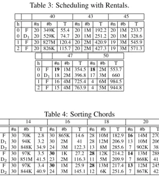
Table 3: Scheduling with Rentals.
40 43 45 h #n #b T #n #b T #n #b T 0 F 20 349K 55.4 20 1M 192.2 20 1M 233.7 0 D1 20 529K 74.7 20 1M 251.2 20 1M 328.6 1 F 20 827M 120.4 20 2M 420.9 19 3M 545.9 2 F 20 826K 115.7 20 2M 427.3 19 3M 571.3 47 50 h #n #b T #n #b T 0 F 19 1M 354.5 18 2M 553.7 0 D1 18 2M 396.8 17 3M 660 1 F 16 4M 725.4 4 6M 984.5 2 F 15 4M 763.9 4 5M 944.8
Table 4: Sorting Chords
14 16 18 20 h #n #b T #n #b T #n #b T #n #b T 0 F 30 70K 2.8 30 865K 14.6 28 10M 182.9 16 14M 270.4 0 D1 30 94K 3.2 30 2M 41 28 12M 206.9 13 10M 206.8 0 D2 30 848K 34.9 24 3M 122.3 13 8M 285.6 7 902K 38.7 1 F 30 97K 3.5 30 1K 27.2 28 12K 214.2 14 13M 288.2 1 D2 30 851M 41.5 23 2M 116.3 11 5M 209.9 7 868K 41.5 2 F 30 97K 3.4 30 1M 25.9 28 13M 217.4 13 12M 245.5 2 D2 30 844K 40.9 24 3M 145.1 12 6K 251.6 7 867K 42.8
generated instances having a fixed length of sub-sequences of size 20 (i.e., len = 20), 50% as a probability of posting an Amongconstraint for each (i, j) s.t. j ≥ i+5 in the sequence. Each set of instances corresponds to a unique sequence size ({40, 43, 45, 47, 50}) and 20 different seeds. We summarize these tests in table 3. Results with decomposition are very poor. We therefore consider only the propagator in this case. 2 Sorting Chords. We need to sort n distinct chords. Each chord is a set of at most p notes played simultaneously. The goal is to find an ordering that minimizes the number of notes changing between two consecutive chords. The full descrip-tion and a CP model is in [Petit, 2012]. The main difference here is that we build a Pareto frontier over two cost variables. We generated 4 sets of instances distinguished by the num-bers of chords ({14, 16, 18, 20}). We fixed the length of the subsequences and the maximum notes for all the sets then change the seed for each instance.
Tables 2, 3 and 4 show that best results were obtained with our propagators (number of solved instances, average back-tracks and CPU time over all the solved instances1). Figure 4
confirms the gain of flexibility illustrated by Figure 1 in Sec-tion 2: allowing h = 1 variable with a low cost value into each sequence leads to new solutions, with significantly lower values for the target variable yc.
6
Conclusion
We have presented flexible tools for capturing the concept of concentrating costs. Our contribution highlights the expres-sive power of constraint programming, in comparison with other paradigms where such a concept would be very difficult to represent. Our experiments have demonstrated the effec-tiveness of the proposed new filtering algorithms.
1
While the technique that solves the largest number of instances (and thus some harder ones) should be penalized.
References
[Dasgupta et al., 2006] S. Dasgupta, C.H. Papadimitriou, and U.V. Vazirani. Algorithms. McGraw-Hill, 2006.
[De Clercq et al., 2011] A. De Clercq, T. Petit,
N. Beldiceanu, and N. Jussien. Filtering algorithms
for discrete cumulative problems with overloads of resource. In Proc. CP, pages 240–255, 2011.
[Narodytska et al., 2013] N. Narodytska, T. Petit, M. Siala, and T. Walsh. Three generalizations of the focus con-straint. Technical report, Avalaible online from CoRR, 2013.
[Pesant and R´egin, 2005] G. Pesant and J.-C. R´egin. Spread: A balancing constraint based on statistics. In Proc. CP, pages 460–474, 2005.
[Petit and Poder, 2008] T. Petit and E. Poder. Global propa-gation of practicability constraints. In Proc. CPAIOR, vol-ume 5015, pages 361–366, 2008.
[Petit and R´egin, 2011] T. Petit and J.-C. R´egin. The ordered distribute constraint. International Journal on Artificial Intelligence Tools, 20(4):617–637, 2011.
[Petit, 2012] T. Petit. Focus: A constraint for concentrating high costs. In Proc. CP, pages 577–592, 2012.
[R´egin, 1996] J.-C. R´egin. Generalized arc consistency for global cardinality constraint. In Proceedings of the 14th National Conference on Artificial intelligence (AAAI’98), pages 209–215, 1996.
[Schaus et al., 2007] P. Schaus, Y. Deville, P. Dupont, and J-C. R´egin. The deviation constraint. In Proc. CPAIOR, volume 4510, pages 260–274, 2007.
[Schaus et al., 2009] P. Schaus, P. Van Hentenryck, and J-C. R´egin. Scalable load balancing in nurse to patient assign-ment problems. In Proc. CPAIOR, volume 5547, pages 248–262, 2009.