Deliverable D 2.2
Scenario 1: Best-case
15/02/2017
BRAIN-TRAINS
Transversal assessment of new
intermodal strategies
WP2: Optimal corridor and hub
development
Christine Tawfik, Martine Mostert and Sabine Limbourg QuantOM (HEC-ULg)
BELGIAN RESEARCH ACTION THROUGH
INTERDISCIPLINARY NETWORKS
CONTENTS
CONTENTS ... 2
INTRODUCTION ... 3
1. HYPOTHESES ... 4
1.1. SCENARIO PARAMETERS ... 4
1.2. OTHER OPERATIONAL PARAMETERS ... 4
2. MODELLING APPROACH ... 5
2.1. SERVICE NETWORK DESIGN ... 5
2.2. JOINT DESIGN AND PRICING ... 6
3. RESULTS AND DISCUSSION ... 7
3.1. SERVICE NETWORK DESIGN ... 7
3.2. JOINT DESIGN AND PRICING ... 9
4. CONCLUSIONS AND PERSPECTIVES ... 14
REFERENCES ... 16
INTRODUCTION
WP2: Optimal corridor and hub development aims at providing tools from the operations
research domain, in order to highlight the potential efficiency of intermodal rail transport in Belgium. The objective of this package is also to give more insight on the decision-making process of the different stakeholders in the intermodal transport chain. The methods are based on the area of expertise of optimization, which aims at translating a managerial problem into a mathematical model that should be optimized. The main components of the methodology consist in:
1) Identifying the managerial problem,
2) Modelling the problem using mathematical programming, 3) Computing the solutions, and
4) Translating the scenarios.
As previously defined in deliverable D1.3, the general goal of the scenarios, within the present research context, is to identify the impact of different plausible situations on the future development of intermodal rail transportation, principally in Belgium. The difference between offering insights into the future, the main scope of the developed scenarios, and attempting to forecast its exact nature is specially highlighted.
As far as WP2 is concerned, the aim is to provide guidelines and outlooks as to the effect of certain operational factors on the competitiveness and the future success of intermodal transport, measured in agreed upon and quantified terms. Indeed, in previous deliverables, the project proposed different important parameters to consider when dealing with intermodal and rail transport in Belgium. These parameters were retrieved out of a SWOT analysis, and selected based on their relevance and plausibility by a panel of experts, using the so-called Delphi method. Different values have been assigned to each parameter, according to the scenario that is used (best-case, worst-(best-case, middle-case).
Throughout this document, our developed models will be tested according to the best-case
scenario values. We essentially adopt two main views: domestic scale, where only national flows
within Belgium are considered, and European scale, where Belgium is regarded as a main start/end point of the flows. Both real and fictitious situations inspired by real life are considered. In what follows, we elaborate on the elements considered for the scenario analysis, the models invoked, the obtained results for the best-case scenario and the foreseen perspectives with respect to the next scenario cases and potential enhancements.
1. HYPOTHESES
1.1.
SCENARIO PARAMETERS
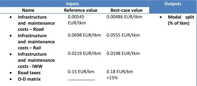
In accordance to the goals set by the White Paper from the European Commission (2011), the best-case scenario is designed to be in line with the desired 30% shift by the year 2030, carried by both the government and the sector. Based on the realized SWOT analysis for each WP, the results are translated into a selection of crucial scenario elements and corresponding parameters and values, validated by the panel of experts of the BRAIN-TRAINS project. Table 1 shows the considered inputs and outputs for WP2, among the total list of scenario parameters, together with the calculated reference- and best-case values of the inputs.
Table 1: Inputs and outputs from the considered scenario parameters
Inputs Outputs
Name Reference value Best-case value
Infrastructure and maintenance costs – Road Infrastructure and maintenance costs – Rail Infrastructure and maintenance costs - IWW Road taxes O-D matrix 0.00545 EUR/tkm 0.0698 EUR/tkm 0.0219 EUR/tkm 0.15 EUR/km ___________ 0.00486 EUR/tkm 0.0555 EUR/tkm 0.0198 EUR/tkm 0.18 EUR/km +15% Modal split (% of tkm)
SOURCE:OWN COMPOSITION, BASED ON DELIVERABLE D1.3
The infrastructure and maintenance costs, as stated in CE Delft (2010) comprise: the construction costs, the maintenance and operational costs and the land use costs. The study further provides a fixed and variable parts division of the costs.
1.2.
OTHER OPERATIONAL PARAMETERS
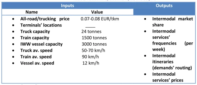
In addition to the above stated parameters, other elements are considered as well to establish necessary operational hypotheses and elements throughout the model runs. The values are based on the norms applied in real life situations according to the collected industry information. Table 2 presents those input parameters that were not explicitly stated among the scenario elements, their selected values (where applicable), as well as additional calculated outputs.
Table 2: Additional operational inputs and outputs
Inputs Outputs
Name Value
All-road/trucking price 0.07-0.08 EUR/tkm Terminals’ locations ____
Truck capacity 24 tonnes Train capacity 1500 tonnes IWW vessel capacity 3000 tonnes Truck av. speed 50-70 km/h Train av. speed 90 km/h Vessel av. speed 12 km/h
Intermodal market share Intermodal services’ frequencies (per week) Intermodal itineraries (demands’ routing) Intermodal services’ prices SOURCE:OWN COMPOSITION
We consider two cases for the terminals’ locations parameter. First, at the domestic Belgian level, the locations are aggregated to the NUTS 3 level based on the setup by Macharis et al. (2009). Second, at the whole European level, we refer to the Agora’s Europe Database and include 13 terminals across the continent. As for the stated modes’ speeds, average cases are assumed for simplification purposes, while acknowledging the existing speed variances in terms of the chosen connections and travelled regions. This is especially valid for the rail freight part; for instance, on the Scandinavian-Mediterranean rail corridor, a requirement is set to attain an operating speed of 100 km/h. However, some sections in Austria only allow 80 km/h due to mountain rail operations. Other speed restrictions for wider bundle of sections are experienced in Italy as well (European Commission, 2014). Furthermore, an assumption is made that freight trains are principally scheduled during the night, hence face low congestion levels.
2. MODELLING APPROACH
Our methods are based on the area of expertise of Mathematical Programming, which aims at translating a managerial problem into a mathematical model, within an optimization framework. We address a tactical, medium-term decision horizon, from an economic perspective (i.e.: no environmental impact involved). The decision maker is namely an intermodal transport operator/service provider. The model is developed and results are analysed over two stages: Service
Network Design and Joint Design and Pricing models.
2.1.
SERVICE NETWORK DESIGN
In order to gain insights about the costs influence on the partition of the flows over the modes of transportation in the network, we start by considering a tactical intermodal service network design problem, from the perspective of a transport service provider operating on a road-rail-IWW network. The decisions to be taken are two-fold: (1) the frequencies of the services over a
certain period of time, typically a week; (2) optimal demands’ routing over the service network. A static case is assumed, where the demands are fixed, as well as the underlying physical network, including the terminals’ locations, throughout the decision process. The following constraints are particularly taken into account:
The total demands should be satisfied and/or delivered by the intermodal services. The services’ capacities are not to be exceeded by the transported volumes. Round long-haul services (>300 km) are enforced, for resource balancing purposes. An itinerary is not to be used, unless a certain fraction of the demand is sent over it
(i.e.: ensuring a minimum utilization).
At a pre-processing stage, a recursive algorithm is designed with the purpose of generating, for each O-D pair, a set of feasible itineraries formed of defined intermodal services. Feasibility is meant in the context of geographical feasibility, mode succession and total length with respect to all-road paths. Mathematically, the model follows the original path-based service network design formulation by Crainic (2000), with an adaptation to the intermodal application context.
2.2.
JOINT DESIGN AND PRICING
At a second stage, we consider an approach that addresses intermodal service prices as explicit decision variables. In particular, we highlight the non-trivial tradeoff between the generated revenues through the collected tariffs and the cost expenses through the operated services; a service performance can be increased, and thus more customers attracted, at the expense of additional operating costs, and vice versa. This implies that the demand volumes are no longer fixed; instead, they depend on the decisions taken by the intermodal service provider.
As a demands’ representation methodology, we adopt the bilevel programming framework. Bilevel programming is essentially inspired by the game-theoretic concept of Stackelberg games (Stackelberg, 1952). It denotes two sequential layers of players: a leader and follower(s). The leader has the precedence privilege of strategy selection, while being able to fully anticipate the rational reaction of the followers to his chosen decisions. The solution (or the chosen strategy) is decided upon by working it backwards; the game is thus played from the point view of the leader. Stackelberg games are first introduced into mathematical programming under the self-explanatory name of “mathematical programs with optimization problems in the constraints”, later known as “bilevel programs”. We observe a similar intrinsic hierarchy in the problem’s definition; first the intermodal operator chooses his services’ pricing and design strategy, while, afterwards, the target shippers optimally react to those decisions by choosing (or not) the offered services. The corresponding bilevel intermodal service design and pricing model can thus be constructed as table 3 shows.
Table 3: Bilevel structure of the joint design and pricing model
Upper level (leader) Lower level (followers)
Decision maker: Intermodal operator/service provider. Decisions:
Services’ prices. Services’ frequencies. Objective: Profit maximization. Constraints:
Services’ capacities are not to be exceeded. Round long-haul services
are enforced.
Decision maker: Shipper firms. Decisions:
Demand volumes on leader’s (intermodal) itineraries.
Demand volumes on
competition (= all-road itinerary).
Objective: Costs minimization. Constraints:
All demands’ are delivered.
SOURCE:OWN COMPOSITION
The model is based on the main bilevel joint pricing and design structure as presented by Brotcorne et al. (2008). The costs from the followers/shippers’ perspective are primarily represented in the prices they are charged for the acquired transport services. Hence, we make the assumption throughout the model development that the competition, represented in trucking services, is able to accommodate all the demands of every shipper firm. It is thus ensured that the leader/intermodal operator is prevented from setting infinite tariff schedules on his services. It is equally important to assume that the competition shows no price change throughout the decision process.
3. RESULTS AND DISCUSSION
In this section, we concentrate on showing the results for every stage of the modelling. The effects of certain parameters’ changes on the intermodal market share, and consequent modal split, are discussed, according to reference- and best-case scenario developments.
3.1.
SERVICE NETWORK DESIGN
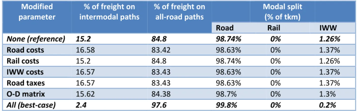
Starting from an O-D matrix of Belgium comprising 302 commodities/shipping demands, all-road paths are enabled for each O-D pair and different scenario elements are changed to their best-case values in order to draw conclusion on the flows partition on the different transport modes, if the costs of operating services become the only considered choice criterion. The first row in table 4 shows the result when all the parameters are tuned to the reference scenario. In the subsequent rows, we refer to the parameter whose value is changed to the best-case scenario values, in order to test the effect and significance of each parameter separately until we arrive, at the last row, where all parameters’ values follow those defined in the best-case scenario.
Table 4: Influence of the best-case parameter values on a costs-driven intermodal shares Modified parameter % of freight on intermodal paths % of freight on all-road paths Modal split (% of tkm)
Road Rail IWW
None (reference) 15.2 84.8 98.74% 0% 1.26% Road costs 16.58 83.42 98.63% 0% 1.37% Rail costs 15.2 84.8 98.74% 0% 1.26% IWW costs 16.57 83.43 98.63% 0% 1.37% Road taxes 16.57 83.43 98.63% 0% 1.37% O-D matrix 15.62 84.38 98.7% 0% 1.3% All (best-case) 2.4 97.6 99.8% 0% 0.2% SOURCE:OWN COMPOSITION
It is understandable that intermodal transport becomes highly dominated by all-road transport due to the fact that we only consider here flows within Belgium (<300 km); a breakeven distance for intermodality’s favour is not reached. A general remark on the above results is that even in the case that intermodal transport is attracting some flows; rail still does not get any shares despite the best-case scenario changes. A possible interpretation for this can be the relatively high fixed costs for rail (0.0541 EUR/tkm), in comparison to those of IWW (0.0205 EUR/tkm), which makes it hard to compensate the operation of a new rail service. Among all the considered parameters, it is evident that the best-case values of the road costs, IWW costs and road taxes have the highest influence. Despite the previous remark, when all values are changed collectively to the best-case scenario, a negative impact is observed on the intermodal share and modal split (last row). This shows that, in the case of increasing shipping demands, the slight decrease in all-road costs attracts most flows, even when combined with a greater decrease in the remaining rail and IWW costs. It equally suggests that the increasing road taxes, due to their presence in the pre- and post-haulage parts in the intermodal transport chain, deter more flows from intermodal paths than it does from all-road paths.
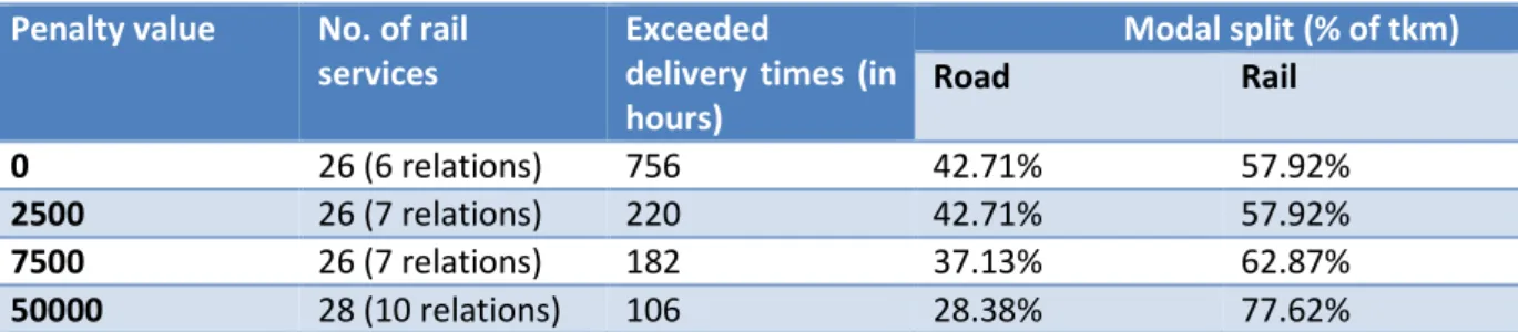
Using the same model, the costs’ scope is generalized to account for service quality aspects, namely, transit time, which will potentially become pronounced on large corridors. The longer-than-necessary delivery times are penalized in the objective function by a changing value, alongside the costs minimization. The shipping demands are extended to long-distance O-D pairs across Europe having 73 commodities, inspired by the announced service connections of a certain intermodal operator. Driven by the data availability at the European level, only road-rail connections are considered for intermodal paths. In order to render the model computationally tractable, rail distances are calculated based on average increases from the equivalent road distances. No all-road paths are enabled, and tests are conducted by altering the transit time penalty value and observing the change in modal split for road (in pre- and post-haulage) and rail (in long-haulage). The reference values of the remaining parameters are considered.
Table 5: Influence of generalized costs on modal split in road-rail paths Penalty value No. of rail
services
Exceeded
delivery times (in hours) Modal split (% of tkm) Road Rail 0 26 (6 relations) 756 42.71% 57.92% 2500 26 (7 relations) 220 42.71% 57.92% 7500 26 (7 relations) 182 37.13% 62.87% 50000 28 (10 relations) 106 28.38% 77.62% SOURCE:OWN COMPOSITION
As shown by table 5, the higher the weight is put on the service performance, described in duration, the more the rail service lines, and the less the transport chain parts carried by road. This may seem counter-intuitive at the outset, as the traditional picture of intermodal transport casts an impression of complicated operations and long transit and transfer times. Even though the speed of a freight train can equal that of a conventional passenger train, the numerous stops imposed on freight trains, as well as the experienced arrival delays, often reduce their commercial door-to-door speed, resulting in supply chain disruptions further down the line. This is, in part, true as the considered model does not fully express the waiting times at the terminals due to delays and consequent missed connections, which are repeatedly reported by the involved actors. However, at an ideal situation, which everyone opts to achieve, the model shows that it is more beneficial, from the service quality point of view, to increase the rail, terminal-to-terminal fast service lines for long distances. This implies a better connected rail network for continental shipping demands, hence, a minimization of the road parts in intermodal itineraries, and ultimately a minimization of transfers along the transport chain. An illustration of the above results on the European map is attached in Appendix 1. The obtained rail connections do not mimic, by any means, the existing EU rail freight corridors in terms of routing choices; they rather show the results of weighing the balance between the modes’ operating costs and the estimated service durations. Thus, a further enhancement of the model could potentially be to take certain rail freight corridors as a starting point for the service design analysis of the considered regions in Europe (e.g., the Rhine-Alpine corridor and the North Sea-Mediterranean corridor) and represent suggested connection frequencies with respect to actually established ones. Nevertheless, incorporating such a realistic dimension implies a considerable computational overhead.
3.2.
JOINT DESIGN AND PRICING
At this second stage, we intend to show the results for the more realistic case, when the demands are no longer fixed and assigned to intermodal paths. Instead, we consider a market where shippers have the choice to send their demands between two available options: an all-road itinerary with a fixed price and intermodal itineraries belonging to a single service provider. A combination of both, and/or of more intermodal itineraries is possible. As previously explained, the problem is depicted as a hierarchical game, played from the perspective of the intermodal service provider, deciding on the design the services, as well as their assigned prices. The same O-D matrix as in the
previous European case study is considered, as well as the same infrastructure at the level of the road and rail physical networks. We begin by showing in figures 1 (a) and 1 (b), for the reference case scenario, the effect of increasing all-road prices and market size, represented in the number of commodities, on the resulting intermodal market share.
Figure 1: Effect of all-road/trucking prices and market size on the intermodal market share (a) (b)
SOURCE:OWN COMPOSITION
It is evident from the graphs that intermodal transport would benefit from increasing competition’s trucking price as well as from increasing the market size constituted of potential shippers. Indeed, a higher competition’s market price implies a higher ceiling for the intermodal services’ prices as well, giving intermodal service providers a bigger room, from the business point of view, to make up for the money invested in operating the services, hence, justify offering more services and attract a larger market. Likewise, an increasing market size offers more opportunities for bundling flows and achieving higher load factors without a big cost increase.
In what follows, we proceed by showing, in table 6, the effect of the change in parameter values, from the reference to the best-case scenario, on the intermodal market share, modal split, as well as the profit margin. The all-road/trucking price is fixed to be 0.08 EUR/tkm throughout the tests; a value decided upon according to market price investigations. A total demand of 73 commodities is considered, as well as a rail service unit constituted of 2 trains (3000 tonnes). Note that, due to the unavailability of actual demand data at the European level, a hypothetical case is examined for comparison purposes, inspired by typical intermodal operators’ announced relations, where the tests do not impose any maximum bound on the pre- and post-haulage distances within the road-rail intermodal connections.
0.00 0.02 0.04 0.06 0.08 0.10 0 20 40 60 80 100 Marke t Share (%)
All-road price (€/ton.km)
0 10 20 30 40 50 60 70 80 0 20 40 60 80 100 Marke t Share (%) No. of commodities
Table 6: Influence of the best-case parameter values on profitability-driven intermodal shares Modified parameter Intermodal market share (% of tkm) Trucking market share (% of tkm)
Modal split Profit (% of tkm) margin
Road Road Rail
(total path) (pph) None (reference) 87.33 12.67 12.67% 41.93% 45.4% 41% Road costs 87.41 12.59 12.59% 42.94% 45.36% 41.5% Rail costs 87.39 12.61 12.61% 41.95% 45.44% 51.6% Road taxes 87.39 12.61 12.61% 41.95% 45.44% 40% O-D matrix 84.77 15.23 15.23% 41.77% 43% 42% All (best-case) 93.64 6.36 6.36% 40.43% 53.21% 47.2% SOURCE:OWN COMPOSITION
The above results are obtained with an acceptable optimality gap of 1-2%. They obviously show that the most significant of all instruments, in terms of profit margin advantage, are the rail costs. Although the increasing O-D flow matrix has, in fact, a negative effect on the intermodal market share, it does not harm the profit margin. It is equally noticeable that the collective application of all the parameter values of the best-case scenario drives the highest improvement on the intermodal market share and a sufficiently better profit margin. In order to get closer to the real-life intermodal transport chains, we impose an upper bound parameter on the total distance run by road in an intermodal itinerary. The corresponding change in intermodal market share, as well as the profit margin is plotted in Figure 2 against the different values of road distance limit.
Figure 2: Impact of the distance done by road on the intermodal transport competitiveness (a) Market share
SOURCE:OWN COMPOSITION -10 0 10 20 30 40 50 60 70 80 90 0 100 200 300 400 M ar ke t sh ar e ( % ) Distance by road (Km) Reference Best case
(b) Profit margin
SOURCE:OWN COMPOSITION
Obviously, the best-case scenario dominates the reference scenario for all considered road distances, in terms of both the market share and the profit margin. As shown in Figure 2(a), the market share in both scenarios undergoes a sharp change, with visible varying severity, at approximately the same road distance (>100 km), after which, it stabilizes around the same values. In Figure 2(b), however, the profit margin in the best-case scenario is stabilized throughout a road distance variation of 300 km, while that of the reference scenario demonstrates a continuous increase, starting from 200 km, until it eventually converges with the best-case result. The above apparently suggests the sensitivity of the conditions imposed on the intermodal paths’ formation, especially in terms of the road parts’ distances, on the competitiveness and profitability of intermodal freight services in a market of scattered demands. As the conditions become looser, the ability of intermodal operators to better tailor their services’ according to the market structure and demands’ locations tends to acquire more flexibility.
Finally, it is often argued about the significance of the rail subsidies on the success of the intermodal transport as a lucrative business, especially in the first stages. Table 7 shows the effect of this parameter, in both the reference and best-case scenario, on the rate of success and market competitiveness of intermodal transport. We consider a moderate limit of 250 km on the distance of the road parts in all intermodal transport itineraries, as well as a rail service unit constituted of a single train (1500 tonnes). To decide on the relevant subsidy levels to be experimented, we analyse the profit margin structure of the intermodal service provider (leader).
𝑃𝑟𝑜𝑓𝑖𝑡 𝑚𝑎𝑟𝑔𝑖𝑛 = 𝑅𝑒𝑣𝑒𝑛𝑢𝑒𝑠 − 𝐶𝑜𝑠𝑡𝑠 𝑅𝑒𝑣𝑒𝑛𝑢𝑒𝑠 = 𝐶𝑜𝑙𝑙𝑒𝑐𝑡𝑒𝑑 𝑡𝑎𝑟𝑖𝑓𝑓𝑠 + 𝑆𝑢𝑏𝑠𝑖𝑑𝑖𝑒𝑠 𝑝𝑒𝑟 𝑑𝑖𝑠𝑡𝑎𝑛𝑐𝑒 − 𝐹𝑖𝑥𝑒𝑑 𝑐𝑜𝑠𝑡𝑠 − 𝑉𝑎𝑟𝑖𝑎𝑏𝑙𝑒 𝑐𝑜𝑠𝑡𝑠𝐶𝑜𝑙𝑙𝑒𝑐𝑡𝑒𝑑 𝑡𝑎𝑟𝑖𝑓𝑓𝑠 + 𝑆𝑢𝑏𝑠𝑖𝑑𝑖𝑒𝑠 𝑝𝑒𝑟 𝑑𝑖𝑠𝑡𝑎𝑛𝑐𝑒 -5 0 5 10 15 20 25 0 100 200 300 400 Pr o fi t m ar gi n ( % ) Distance by road (Km) Reference Best case
= (𝑃𝑟𝑖𝑐𝑒𝑠×𝐷𝑒𝑚𝑎𝑛𝑑𝑠) + (𝑆𝑢𝑏𝑠𝑖𝑑𝑖𝑒𝑠 ×𝐹𝑟𝑒𝑞𝑢𝑒𝑛𝑐𝑦 ) − (𝐹𝑖𝑥𝑒𝑑 𝑐𝑜𝑠𝑡𝑠 ×𝐹𝑟𝑒𝑞𝑢𝑒𝑛𝑐𝑦) − (𝑉𝑎𝑟𝑖𝑎𝑏𝑙𝑒 𝑐𝑜𝑠𝑡𝑠×𝐷𝑒𝑚𝑎𝑛𝑑𝑠) (𝑃𝑟𝑖𝑐𝑒𝑠×𝐷𝑒𝑚𝑎𝑛𝑑𝑠) + (𝑆𝑢𝑏𝑠𝑖𝑑𝑖𝑒𝑠 ×𝐹𝑟𝑒𝑞𝑢𝑒𝑛𝑐𝑦 )
We observe from the above formulas that, for a certain service frequency level, an increase in subsidies would imply a proportional increase in the consequent profit and profit margin. This increase would continue until a subsidy level is reached that justifies the offering of new services (increase in frequency) and make up for the related costs, in particular, the fixed components. Therefore, we choose the tested subsidy levels, with respect to the considered costs in each scenario (table 1).
Table 7: Impact of rail subsidies on the success of intermodal transport business (a) Reference scenario
Subsidy level (EUR/km) Market share (% of tkm) Profit margin (%) No. of rail services Average load factor (%) 0 66.19 6.8 14 99.2 5 71.79 10.1 16 99.3 10 71.79 13.71 16 99.3 20 71.79 20.2 16 99.3 25 81.32 20.4 20 94 30 81.32 23.3 20 94 35 81.32 26 20 94 40 92.39 24 24 86.7 SOURCE:OWN COMPOSITION (b) Best-case scenario Subsidy level (EUR/km) Market share (% of tkm) Profit margin (%) No. of rail services Average load factor (%) 0 74.56 24.11 20 98.5 2 83.05 22.74 22 96.2 5 88.78 23.15 24 94.2 7 88.78 24.54 24 94.2 10 93.62 24.98 26 91.9 12 93.62 26.31 26 91.9 15 96.45 27.3 28 89.9 25 96.45 33.15 30 83.9 SOURCE:OWN COMPOSITION
Tables 7 (a) and (b) both show the general positive impact of applying subsidies on the competitiveness and profitability of intermodal transport, though with different intensity and consequences. For instance, we notice that the market share, as well as the load factor, is more sensitive to the small changes in the subsidy levels in the best-case scenario, than it is in the reference scenario, especially at the first stages (0-10 EUR/km). This can be partially attributed to the difference in costs to be compensated between the scenarios. On the other hand, the profit margin shows a continuous and faster increase in the reference scenario, when compared to the steadier
behaviour in the best-case scenario, for the same subsidy levels (0-25 EUR/km). A possible interpretation of this previous observation in the best-case scenario can be the already advantageous position it is starting with and the greater ability for the subsidies to help offer more services, hence more costs and a slower increase of profit, rather than a direct resonance in costs-free revenues. Furthermore, as opposed to the reference scenario, market position stagnation is reached in the best-case scenario with relatively high levels of subsidies (>10 EUR/km).
4. CONCLUSIONS AND PERSPECTIVES
In the context of testing the impact of certain instrumental changes on the intermodal freight transport and drawing insights about its potential future, we model a medium-term planning problem from the perspective of a typical intermodal operator. The decisions are two-fold: the prices of the offered freight services and the design the service network, in terms of the frequencies and demand routing. The model follows the structure of a bilevel joint design and pricing model. The problem is addressed in two stages. First, a case of fixed demands is considered, where the pricing decisions are omitted and conclusions are made with respect to the operating costs. Second, demands are explicitly modelled as subject to the services’ prices and design decisions, by expressing the rational behaviour of the target shipper customers within a hierarchical Stackelberg game model. A competition, represented in trucking services, is always assumed to be available.
Based on the experiments and obtained results in each case study, we summarize the most notable conclusions in the following points:
From a pure costs perspective, intermodal transport is more expensive to offer than all-road transport for distances < 300 km (the Belgian case), with a clear favouring of IWW over rail transport, potentially attributed to the high rail fixed costs.
Despite the observation that the best-case values of the road costs, IWW costs and road taxes, separately, yield a positive effect, the collective application of the best-case scenario parameters results in an overall more costly position for intermodal transport.
At the European level, from a generalized costs perspective, a weight on the service quality can give an advantage for rail transport in terms of minimizing the road parts and increasing the terminal-to-terminal rail services, within the intermodal itineraries, in order to achieve faster connections.
In the case of jointly optimizing the service design and pricing decisions, a directly proportional relation exists between the intermodal market share and the corresponding competition’s trucking price and market size.
The best-case scenario suggests an improvement of the intermodal market share with respect to the reference scenario, with a particularly significant impact of the new rail costs parameter values on the related profit margin.
Both the competitiveness and profitability of intermodal transport are found sensitive to the intermodal paths’ structure, namely, in terms of the distance limits imposed on the road parts. Higher limits imply a greater opportunity to cover a larger market and generate a higher profit.
In what concerns the rail subsidies, rail-based intermodal transport, in the future best-case scenario, can benefit from relatively less subsidies to rapidly cover more market, up until a certain level. Afterwards, more subsidies imply an increased profit, though less load factors.
In the next scenarios’ analysis, we intend to refine our methodology, in terms of increasing the realism of the model. What we considered this far assumes a theoretical, nearly ideal case, where decisions are made in the framework of mathematical optimization systems. In real-life situations, the general behavioral assumption is that shippers seek to minimize their total logistics costs, and thus increase their respective utility of freight modes. This is frequently a process that comprises a non-uniformity of the service quality perception among the shippers and imperfect and/or missing significant information. In order to incorporate this randomness dimension, the solution, as proposed by Ben-Akiva et al. (2013), is to combine discrete choice methods with the minimization of total logistics costs, in the same way that utility maximization is modeled for individuals’ choice behavior in passenger traffic. The idea is to ultimately integrate this methodology in the reaction of the followers within the bilevel pricing and design model, as presented above. Additionally, we highlight the particular importance of considering more realistic cost components and shipping demands, as closely as possible to those experienced by typical intermodal service providers on the European network, in order to be capable of giving back relevant practical insights for the future of intermodality.
REFERENCES
Agora, intermodal terminals database. http://www.intermodal-terminals.eu/
Ben-Akiva, M., Meersman, H., Van De Voorde, E., 2013. Freight transport modelling. ISBN: 978-1781902851.
Brotcorne, L., Labbé, M., Marcotte, P., Savard, G., 2008. Joint design and pricing on a network. Operations Research, vol. 56, no. 5, pp. 1104-1115.
CE Delft, INFRAS, Alenium and HERRY Consult, External and infrastructure costs of freight transport Paris-Amsterdam corridor - Deliverable 1 – Overview of costs, taxes and charges, CE Delft, Delft 2010.
Crainic, T. G., 2000. Service network design in freight transportation. European Journal of Operational Research 122, pp. 272-288.
European Commission, 2014. Scandinavian-Mediterranean Core Network Corridor Study. Final Report. http://ec.europa.eu/transport/themes/infrastructure/ten-t-guidelines/corridors/corridor-studies_en
Macharis, C., Janssens, G. K., Jourquin, B., Pekin, E., Caris, A. and Crepin, T. (2009). Decision support
system for intermodal transport policy (DSSITP). Science for a sustainable development (SSD).
APPENDIX I – Rail services design results from generalized costs
minimization
The following figures illustrate the results previously shown in table 5, according to the presented order. In each case, 73 commodities/shipping demands are considered. The pinpoints represent the terminals’ locations, while the red lines serve as the resulting rail connections between the terminals. The rail connections do not correspond to connections within the existing EU rail freight corridors; they rather show a suggested rail network in order to obtain the desired balance between the different service factors. This explains the resulting short rail connections throughout central Europe in some penalty cases; deliveries are completed by road connections.
Penalty = 0
Penalty = 7500