Facult´e des Sciences Appliqu´ees
Symbolic Methods for Exploring
Infinite State Spaces
Th`ese pr´esent´ee par Bernard Boigelot
en vue de l’obtention du titre de Docteur en Sciences Appliqu´ees Ann´ee Acad´emique 1997–1998
Abstract
In this thesis, we introduce a general method for computing the set of reachable states of an infinite-state system. The basic idea, inspired by well-known state-space exploration methods for finite-state systems, is to propagate reachability from the initial state of the system in order to determine exactly which are the reachable states. Of course, the problem being in general undecidable, our goal is not to obtain an algorithm which is guaranteed to produce results, but one that often produces results on practically relevant cases.
Our approach is based on the concept of meta-transition, which is a mathematical object that can be associated to the model, and whose purpose is to make it possible to compute in a finite amount of time an infinite set of reachable states. Different methods for creating meta-transitions are studied. We also study the properties that can be verified by state-space exploration, in particular linear-time temporal properties.
The state-space exploration technique that we introduce relies on a symbolic representation system for the sets of data values manipulated during exploration. This representation system has to satisfy a number of conditions. We give a generic way of obtaining a suitable representation system, which consists of encoding each data value as a string of symbols over some finite alphabet, and to represent a set of values by a finite-state automaton accepting the language of the encodings of the values in the set. Finally, we particularize the general representation technique to two important domains: unbounded FIFO buffers, and unbounded integer variables. For each of those domains, we give detailed algorithms for performing the required operations on represented sets of values.
Acknowledgments
I would first like to thank my thesis advisor, Pierre Wolper, for getting me started in the field of verification, and sharing with me his contagious enthusiasm about finite automata. His insightful comments contributed significantly to the content and the presentation of this thesis. Thanks also to the other members of my jury, Daniel Ribbens, Pascal Gribomont, V´eronique Bruy`ere, Pierre-Yves Schobbens, Alain Finkel and Bengt Jonsson, who have accepted to read and evaluate this thesis. It has been a great pleasure for me to work in collaboration with several other people during these last four years. I wish to thank Patrice Godefroid, who signifi-cantly influenced much of the work contained in this thesis. Patrice also contributed to some of the results presented in Chapters 3 to 7, and made possible two exciting stays at Bell Laboratories in 1995 and 1996. Thanks to Bernard Willems, who in-troduced me to some areas of mathematics and most willingly helped me to tackle various problems. The results exposed in Chapter 8 would not be in the present form without the help of Bernard. Thanks also to Louis Bronne and to St´ephane Rassart, who contributed substantially to some of the results presented in Chap-ter 8 and provided me with valuable comments and suggestions. I am also grateful to G´erard C´ec´e and Philippe Louis for their careful reading of Chapter 7.
Thanks to all the people that shared with me their insightful ideas about sym-bolic verification at various conferences and meetings. In particular, I thank Pascal Gribomont, Ahmed Bouajjani, Alain Finkel, Yassine Lakhnech, Hubert Comon, and V´eronique Bruy`ere.
I am grateful to the National Fund for Scientific Research of Belgium (FNRS), which supported me as research assistant (“aspirant”) and research associate (“char-g´e de recherches”).
Finally, thanks to my colleagues Philippe Lejoly, Didier Rossetto, Ulrich Nitsche, Didier Pirottin and Diana Tourko which provided me with an enjoyable work envi-ronment. Thanks also to Edie and Gary, to all my good friends for their support, and — last but not least — to Murielle for her . . . infinite love.
Contents
Abstract iii Acknowledgments v Contents vii Figures xi 1 Introduction 11.1 Overview of the Thesis . . . 5
2 Structured-Memory Automata 7 2.1 Modeling Programs . . . 7 2.2 Semantics . . . 8 2.3 Example . . . 9 2.4 Discussion . . . 11 3 Reachability Analysis 13 3.1 Finite-State Systems . . . 13 3.2 Infinite-State Systems . . . 15
3.2.1 Exploring Infinite Sets of Reachable States . . . 16
3.2.2 Representing Infinite Sets . . . 17
3.3 Symbolic State-Space Exploration . . . 19
3.4 Creating Meta-Transitions . . . 23
3.4.1 Cycle Meta-Transitions . . . 23
3.4.2 Multicycle Meta-Transitions . . . 29
3.5 Dynamic Creation of Meta-Transitions . . . 31
3.6 Example . . . 37 3.7 Discussion . . . 38 4 Properties 43 4.1 Reachability Properties . . . 43 4.2 Deadlock Detection . . . 44 vii
4.3 Temporal Properties . . . 44
4.3.1 Linear-Time Temporal Logic . . . 45
4.3.2 B¨uchi Automata . . . 46
4.3.3 Example . . . 48
4.4 Model Checking . . . 49
4.4.1 Finite-State Systems . . . 49
4.4.2 Infinite-State Systems . . . 51
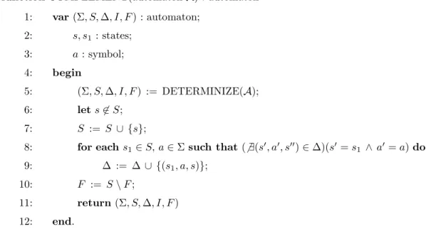
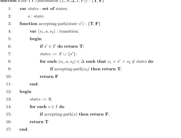
4.5 Testing the Emptiness of SMBAs . . . 53
4.5.1 Expressiveness of Memory Domains . . . 53
4.5.2 Undecidability of the Emptiness Problem . . . 56
4.5.3 Semi-Decision Procedure . . . 56
5 Termination 63 5.1 Undecidability of Termination . . . 63
5.2 Sufficient Conditions . . . 65
5.3 Machines with Only Cycle Meta-Transitions . . . 66
5.3.1 Transition Segments . . . 66
5.3.2 Meta-Transition Segments . . . 67
5.3.3 Number of Segments . . . 68
5.3.4 Summary of Conditions . . . 75
5.3.5 Implementation . . . 76
5.4 Machines with Only Multicycle Meta-Transitions . . . 78
5.4.1 Transition Segments . . . 78
5.4.2 Meta-Transition Segments . . . 78
5.4.3 Number of Segments . . . 79
5.4.4 Summary of Conditions . . . 82
5.5 LTL Model Checking . . . 83
5.5.1 Systems with Only Cycle Meta-Transitions . . . 83
5.5.2 Summary of Conditions . . . 86
5.5.3 Systems with Only Multicycle Meta-Transitions . . . 88
5.5.4 Summary of Conditions . . . 90
5.6 Control Graph Optimization . . . 92
5.6.1 Introduction . . . 92
5.6.2 Loop Optimization . . . 93
5.6.3 Implementation . . . 100
6 Finite-State Representation Systems 105 6.1 Finite-State Automata . . . 105
6.2 Operations on Automata . . . 107
6.2.1 Determinization . . . 107
CONTENTS ix
6.2.3 Closure and Concatenation . . . 109
6.2.4 Set-Theory Operators . . . 114
6.3 Automata as Representations of Sets . . . 120
6.4 Operations on Representable Sets . . . 122
7 Systems Using FIFO Channels 125 7.1 Basic Notions . . . 125
7.1.1 Queue SMAs . . . 125
7.1.2 Turing Expressiveness . . . 126
7.1.3 Queue Decision Diagrams . . . 128
7.1.4 Notations . . . 132
7.2 Elementary Queue Operations . . . 132
7.2.1 Systems with One Queue . . . 133
7.2.2 Systems with Any Number of Queues . . . 134
7.2.3 Sequence of Elementary Operations . . . 140
7.3 Creation of Cycle Meta-Transitions . . . 140
7.3.1 Systems with One Queue . . . 141
7.3.2 Systems with Any Number of Queues . . . 154
7.4 Creation of Multicycle Meta-Transitions . . . 162
7.4.1 Systems with One Queue . . . 164
7.4.2 Systems with Any Number of Queues . . . 173
7.5 Creation of Other Meta-Transitions . . . 176
7.6 Model Checking with Cycle Meta-Transitions . . . 180
7.6.1 Systems with One Queue . . . 180
7.6.2 Systems with Any Number of Queues . . . 183
7.7 Model Checking with Multicycle Meta-Transitions . . . 184
7.7.1 Systems with One Queue . . . 184
7.7.2 Systems with Any Number of Queues . . . 185
7.8 Termination . . . 188
7.8.1 Finiteness of Sets of Queue-Set Contents . . . 188
7.8.2 Precedence Relation . . . 188
7.9 Loop Optimization . . . 192
8 Systems Using Integer Variables 193 8.1 Basic Notions . . . 193
8.1.1 Integer SMAs . . . 193
8.1.2 Turing Expressiveness . . . 195
8.1.3 Number Decision Diagrams . . . 196
8.1.4 Representable Sets of Vector Values . . . 197
8.1.5 Sets that are Representable in Any Basis . . . 207
8.2 Linear Operations . . . 211
8.3 Creation of Cycle Meta-Transitions . . . 213
8.3.1 Overview . . . 213
8.3.2 Algebra and Combinatorics Basics . . . 214
8.3.3 Recognizability of Sets of Complex Vector Values . . . 216
8.3.4 Necessary Conditions . . . 219
8.3.5 Sufficient Conditions . . . 225
8.3.6 Algorithms . . . 226
8.3.7 Linear Operations with Guard . . . 235
8.3.8 Proofs of Auxiliary Results . . . 238
8.4 Creation of Multicycle Meta-Transitions . . . 264
8.5 Model Checking . . . 265
8.6 Termination . . . 272
8.6.1 Finiteness of Sets of Vector Contents . . . 272
8.6.2 Precedence Relation . . . 273 8.7 Loop Optimization . . . 275 9 Conclusions 281 9.1 Summary . . . 281 9.2 Related Work . . . 283 9.3 Future Work . . . 288 Bibliography 289
List of Figures
1.1 Simple infinite-state system. . . 4
2.1 Example of SMA. . . 10
2.2 State space of the example. . . 10
3.1 Breadth-first exploration of a finite state space. . . 14
3.2 Depth-first exploration of a finite state space. . . 15
3.3 Breadth-first exploration of an infinite state space. . . 20
3.4 Depth-first exploration of an infinite state space. . . 22
3.5 Creation of simple-cycle meta-transitions. . . 25
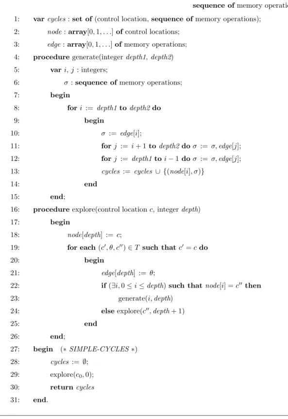
3.6 Computation of all the simple cycles in the control graph. . . 26
3.7 Control graph with 2N transitions and N2N simple cycles. . . 28
3.8 Creation of cycle meta-transitions from syntactic cycles. . . 29
3.9 Creation of multicycle meta-transitions. . . 32
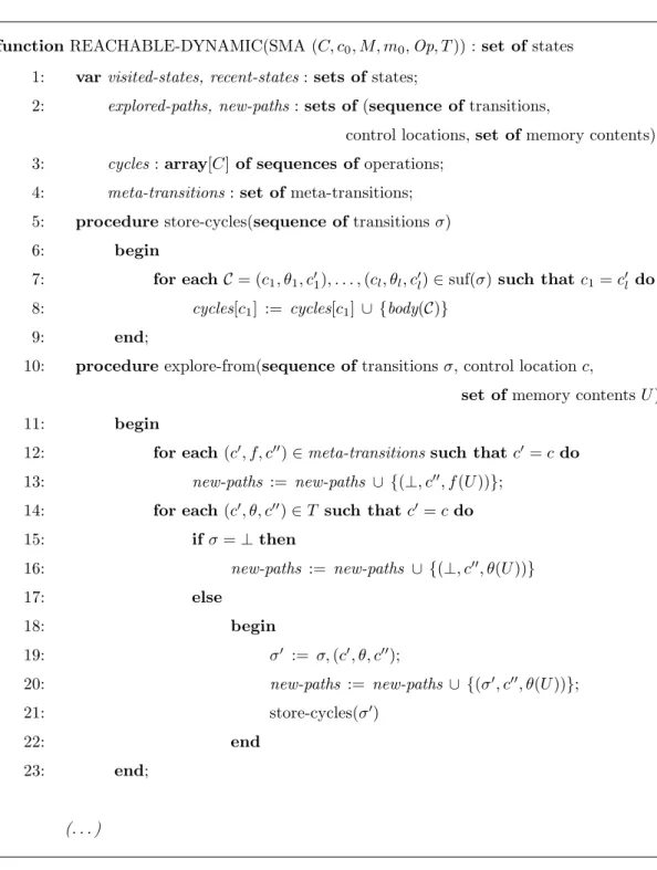
3.10 State-space exploration by dynamic creation of meta-transitions. . . . 33
3.11 State-space exploration by dynamic creation of meta-transitions (con-tinued). . . 34
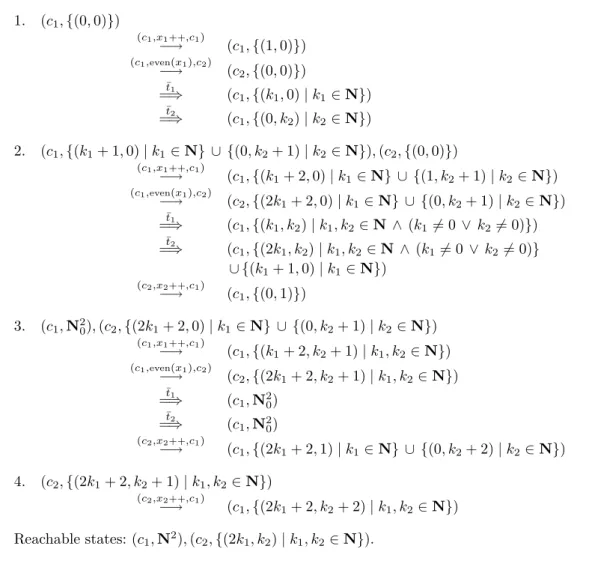
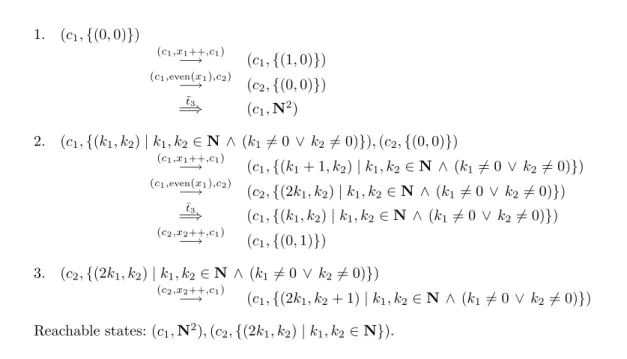
3.12 Example of state-space exploration with simple-cycle meta-transitions. 39 3.13 Example of state-space exploration with multicycle meta-transitions. 40 4.1 B¨uchi automaton. . . 48
4.2 Test of emptiness for SMBAs. . . 59
5.1 SMBA accepting a nonempty language. . . 84
5.2 Test of emptiness for safe SMBAs (with only cycle meta-transitions). 87 5.3 Test of emptiness for safe SMBAs (multicycle meta-transitions). . . . 91
5.4 Example of program with nested loops. . . 93
5.5 Control graph of program with nested cycles. . . 94
5.6 Cycle equivalent to nested loops. . . 95
5.7 Loop optimization for SMBAs. . . 96
5.8 Loop optimization for SMAs. . . 97
5.9 Illustration of loop optimization. . . 98
5.10 Decision procedure for optimizability of a simple cycle. . . 101 xi
5.11 Repeated loop optimizations for SMBAs. . . 103
5.12 Repeated loop optimizations for SMBAs (continued). . . 104
5.13 Repeated loop optimizations for SMAs. . . 104
6.1 Normalization of an automaton. . . 108
6.2 Determinization of an automaton. . . 110
6.3 Minimization of a deterministic automaton. . . 111
6.4 Minimization of a deterministic automaton (continued). . . 112
6.5 Computing the closure of an automaton. . . 113
6.6 Closure of an automaton. . . 113
6.7 Concatenating two automata. . . 114
6.8 Concatenation of two automata. . . 115
6.9 Synchronous product of two automata. . . 115
6.10 Intersection of two automata. . . 116
6.11 Computing the union of two automata. . . 117
6.12 Union of two automata. . . 117
6.13 Complement of an automaton. . . 118
6.14 Difference between two automata. . . 118
6.15 Test of emptiness of the language accepted by an automaton. . . 119
6.16 Test of inclusion between two languages accepted by automata. . . . 120
6.17 Application of an homomorphism to an automaton. . . 121
7.1 Receive operation for a single-queue QDD. . . 133
7.2 Send operation for a single-queue QDD. . . 134
7.3 Image of a single-queue QDD by a sequence of queue operations. . . . 135
7.4 Application of a QDD operation to a specified queue. . . 137
7.5 Send operation for an arbitrary QDD. . . 139
7.6 Receive operation for an arbitrary QDD. . . 139
7.7 Image of an arbitrary QDD by a sequence of queue operations. . . 139
7.8 Effect of repeated applications of APPLY-ONE. . . 142
7.9 Initial states that are provably robust (|σ!| ≥ |σ?|). . . 145
7.10 Initial states that are provably robust (|σ!| < |σ?|). . . 145
7.11 Initial states partitioning (|σ!| ≥ |σ?|). . . 147
7.12 Initial states partitioning (|σ!| < |σ?|). . . 147
7.13 Automaton accepting Si≥i0(L(A α′ i ) ∪ L(A β′ i )). . . 148
7.14 Automaton accepting Si≥i0L(Aγi′) (with |σ!| ≥ |σ?|). . . 149
7.15 Automaton accepting Si≥i0L(A δ′ i ) (with |σ!| ≥ |σ?|). . . 151
7.16 Right blocks. . . 152
7.17 Subroutine APPEND-LOOP. . . 154
7.18 Image of a single-queue QDD by the closure of a sequence of queue operations. . . 155
LIST OF FIGURES xiii 7.19 Image of a single-queue QDD by the closure of a sequence of queue
operations (continued). . . 156
7.20 Image of a single-queue QDD by the closure of a sequence of queue operations (continued). . . 157
7.21 Implementation of META? for sequences of queue operations. . . 161
7.22 Image of a QDD by the closure of a sequence of queue operations. . . 163
7.23 Image of a single-queue QDD by a receive-deterministic multisequence of queue operations. . . 165
7.24 Effect of repeated applications of APPLY-MULTI-ONE. . . 167
7.25 Image of a single-queue QDD by repetitions of a receive-deterministic multisequence of queue operations. . . 168
7.26 Subroutine APPEND-N-MULTI-LOOP. . . 169
7.27 Subroutine APPEND-MULTI-LOOP. . . 169
7.28 Image of a single-queue QDD by the closure of a send-synchronized multisequence of queue operations. . . 170
7.29 Image of a single-queue QDD by the closure of a send-synchronized multisequence of queue operations (continued). . . 171
7.30 Image of a single-queue QDD by the closure of a a send-synchronized multisequence of queue operations (continued). . . 172
7.31 Image of an arbitrary QDD by multisequence of queue operations. . . 174
7.32 Image of an arbitrary QDD by repeated applications of a multise-quence of queue operations. . . 174
7.33 Image of a QDD by the closure of a multisequence of queue operations whose projections are send-synchronized. . . 177
7.34 Creation of multicycle meta-transitions. . . 178
7.35 Image of a QDD by the memory function modeling loss. . . 180
7.36 Set of queue contents to which a sequence can be applied infinitely many times (one queue). . . 182
7.37 Set of queue-set contents to which a sequence can be applied infinitely many times (any number of queues). . . 183
7.38 Set of queue contents to which a send-synchronized multisequence can be applied infinitely many times (one queue). . . 186
7.39 Set of queue contents to which a send-synchronized multisequence can be applied infinitely many times (one queue, continued). . . 187
7.40 Set of queue-set contents to which a multisequence can be applied infinitely many times (any number of queues). . . 187
7.41 Test of finiteness of the language accepted by an automaton. . . 189
7.42 Precedence test for sequences of queue operations. . . 191
8.1 NDD representing U=. . . 200
8.3 NDD representing U+. . . 201
8.4 NDD representing UVr. . . 202
8.5 Projection of an NDD with respect to a vector component. . . 204
8.6 Reordering of an NDD. . . 205
8.7 Application of a linear operation to an NDD. . . 213
8.8 Decision procedure for the preservation of r-definability by the closure of a guardless linear operation. . . 231
8.9 Decision procedure for the preservation of r-definability by the closure of a guardless linear operation (continued). . . 232
8.10 Implementation of META? for guardless linear operations in a given basis. . . 233
8.11 Implementation of META? for guardless linear operations in any basis.234 8.12 Image of an NDD by the closure of a guardless linear operation in a given basis. . . 234
8.13 Image of an NDD by the closure of a guardless linear operation in any basis. . . 235
8.14 Image of an NDD by the closure of a linear operation in a given basis. 239 8.15 Image of an NDD by the closure of a linear operation in any basis. . . 240
8.16 Creation of multicycle meta-transitions in a given basis. . . 266
8.17 Creation of multicycle meta-transitions in any basis. . . 266
8.18 Set of vector values to which a linear operation can be applied in-finitely many times (in a given basis). . . 269
8.19 Set of vector values to which a linear operation can be applied in-finitely many times (in any basis). . . 270
8.20 Set of vector values to which a finite set of linear operations can be applied infinitely many times (in a given basis). . . 271
8.21 Set of vector values to which a finite set of linear operations can be applied infinitely many times (in any basis). . . 271
8.22 Test of finiteness of a set represented as an NDD. . . 272
8.23 Precedence test for linear operations. . . 274
8.24 Computation of a linear operation equivalent to (θ1; θ1+; θ2). . . 278
8.25 Predicate EXISTS-LOOP-EQUIV? for linear operations. . . 279
Chapter 1
Introduction
Because of the rapid progress of computer technology over the last decades, com-puters are now present in a large variety of devices, ranging from home appliances driven by simple microcontrollers to phone switches controlled by massively paral-lel units. Even an increasing number of life-critical systems rely on computers: in modern fly-by-wire aircrafts, control surfaces are actuated by flight computers rather than being mechanically linked to the pilot controls. The consequences of computer system failures have thus become more and more severe. Over the last years, there have been numerous cases of major disturbances and even fatalities caused by com-puter problems [Neu96]. As a chilling example, there have been more than ten fatal computer-related aircraft incidents over the last fifteen years [Neu97].
It is therefore crucial for developers of computer systems to have at their disposal analysis techniques for detecting potential failures before those systems are used. Even for systems which are not life-critical, it is always economically sound to detect design flaws as early as possible in the development process.
A long promoted way of designing correct computer systems is to develop with the system a formal proof of its correctness. This proof is traditionally based on
invariants, which are logic formulas whose truth value provably never changes
dur-ing the possible runs of the system. The correctness of the system is expressed as a logical consequence of an invariant that is initially true. Invariants are written in dedicated logics such as Hoare’s logic [Hoa69] or Dijkstra’s programming calcu-lus [Dij76]. Even though this mathematically appealing approach has occasionally been applied [vLS79, CE81, CM89, Gri93], it inherently suffers from major draw-backs:
• It is costly. Writing a formal proof, even with the assistance of a computerized tool, is not straightforward and may require a significant amount of time, ingenuity, and experience.
• It is not practical. For instance, it is not possible to reuse already existing code if this code was developed without a proof. Even if this does not seem to
be a major restriction for some specific applications, there are many domains in which it is not economically feasible not to reuse parts of existing systems (for instance, banking or phone switching software).
• It is rigid. Even if a system is proved correct with respect to some properties, obtaining a correction proof for other properties may require a complete new study of the system.
An alternative approach is automated verification. Given a computer system, one uses an automatic technique for checking that each execution of the system satisfies some correctness criteria. In practice, this cannot be done while taking into account all the details of the system; indeed, an analysis carried out up to the greatest level of precision would have to deal with the electrical and even chemical phenomena occurring inside the components of the computer. This is far beyond our ambition. The solution is to define some level of abstraction, and write a model, i.e., a formal description of the system at that level of abstraction. In addition, one must also define properties expressing the correctness of the model at that level of abstraction. Properties are often written in dedicated logic formalisms such as temporal logics [Wol86, Wol83, Eme90, MP92]. The analysis simply consists of checking if every execution of the model satisfies all the correctness properties.
The result of the analysis is either the detection of an error, or a guarantee that the model is correct with respect to the properties. In practice, results of the former type are the most interesting ones, because it is often easy to check whether an error in the model corresponds or not to an error in the original system. On the contrary, a guarantee of correctness for the model does not translate into a certainty of correctness for the system, unless lots of hypotheses are assumed. (Nevertheless, such a proof may increase the level of confidence in the system.)
In this thesis, we consider systems modeled as state machines. Intuitively, this modeling scheme is based on the assumption that each run of the system can be described by a (possibly infinite) sequence of discrete state changes. The model then consists of a finite amount of information defining the initial state of the system, as well as all the possible state changes.
A simple way of checking the correctness of such a model is to explore its state space. Roughly speaking, the idea is to check systematically all the possible situ-ations that can occur during the possible executions of the model. If an execution violating a property is found, then a scenario proving that the model is erroneous is produced. If no such execution is found after exploring all the possible situations, then one can deduce that the model is “correct” [Hol88, Hol90]. The main drawback of this approach is that a model can have a very large number of states (meaning that there are a very large number of situations to check). This phenomenon is known as the combinational explosion of the number of states with respect to the size of the model. Tools have been developed for performing exhaustive state-space
3 exploration [HK90, Hol91, DDHY92, FGM+92], and have been successfully used to
detect unsuspected errors in industrial systems [BG96a]. However, their applicabil-ity is still limited to small systems. Simple optimizations of the iterative state-space exploration technique have been proposed in order to broaden the set of analyzable systems [Mor68, WL93, PY97]. Despite some practical advantages inherent to those optimizations, their use does not significantly increase the order of magnitude of the size of the systems that can be handled.
On the other hand, techniques were developed for attacking directly the sources of state-space explosion. A first example is partial-order methods [Val91, GW93, God96], which attempt to limit the explosion caused by the modeling of concur-rency by interleaving [Win84]. The idea consists of exploring only a part of the state space, this part being sufficient for checking the validity of the properties of interest. Another category of techniques tackling state-space explosion are symbolic
methods [BCM+92, McM93]. There, the basic idea is to represent and manipulate
sets of states implicitly (with the help of specific data structures), rather than explic-itly (as enumerations of their components). In this approach, the improvement does not concern the number of states to be explored, but instead the total cost of this exploration. Symbolic methods have been successfully applied to different domains such as hardware circuits [KL93], real-time systems [ACD90, AHH93, HNSY94], and hybrid systems [HH94, Hen96].
The most widely used representation system for symbolic exploration is the
Bi-nary Decision Diagram (BDD) [Bry92]. The idea consists of encoding the elements
of a set as fixed-length words of bits. The set is then represented by a canonical decision diagram – isomorphic to a directed acyclic graph – that recognizes the en-codings of all the elements of the set. This simple and elegant representation has efficient implementations, and can easily be applied to a large class of domains. It does however suffer from an important drawback: BDDs only allow the representa-tion of finite sets. As a consequence, symbolic explorarepresenta-tion with BDDs is limited to the analysis of models with a finite state space.
It is however crucial to be able to analyze models with an infinite state space. Indeed, even though all physically constructible systems are finite in some sense, their size is often way larger than what can be handled by finite-state methods. Modeling such systems as infinite-state systems is then more realistic than artificially bounding their size well below reality. (For instance, a buffer with ten megabytes of capacity is more accurately modeled by an unbounded buffer than by a two-byte buffer.) Another reason is that verification methods can also be used to check the correctness of abstract systems from which real systems can then be derived. It is often more comfortable to reason independently from any limit than to impose an arbitrary upper bound on the size of a system. Finally, it should be stressed that techniques developed for infinite-state systems may remain very powerful for analyzing systems for which the state space is finite but very large. For instance,
programCOUNTER;
1: vari : unbounded integer;
2: begin 3: i := 0; 4: repeat 5: i := i + 2 6: until i = 0 7: end.
Figure 1.1: Simple infinite-state system.
there are systems whose state space is limited by an upper bound (such as the capacity of a communication object), for which the cost of state-space exploration appears to be independent of that bound.
Infinite-state models also have some disadvantages. The main one is that most elementary properties are undecidable for sufficiently expressive classes of mod-els [EN94, Fin94, HKPV95, CFI96, ACJT96, AJ96, Esp97]. This implies that, in general, it is not possible to analyze such systems rigorously, and hence that only partial results can be obtained. Note however that this situation is not very differ-ent in practice from what occurs for finite-state systems, for which the analysis is often impossible due to excessive resource (time or memory) requirements, in spite of a theoretical guarantee that an analysis can always be carried out. Our point of view is that it is more useful to provide a partial solution to an important general problem rather than isolate elegant but not very meaningful subclasses of systems for which a complete analysis is theoretically always possible.
Another drawback of infinite-state models is that the result of their reachability analysis cannot be expressed as the explicit enumeration of all their reachable states. One has thus to resort to symbolic methods for representing implicitly sets of states, as well as to specific techniques for computing infinitely many reachable states in a finite amount of time. This is not very different from what is usually done during program analyses carried out by hand, as illustrated with the Pascal-like program given in Figure 1.1. Even though this program has an infinite state space, it is easily inferred that:
• Each execution of the main loop at Lines 2–6 has the effect of adding 2 to the value of i;
• The values that i can take just before executing Line 6 are exactly all the strictly positive even numbers;
1.1. OVERVIEW OF THE THESIS 5 • The program does not terminate.
This approach can be generalized and automatized. In this thesis, we address the problem of exploring infinite-state spaces with the help of symbolic methods. The results presented here extend and unify those appearing in previous publica-tions [BW94, WB95, BG96b, BGWW97].
1.1
Overview of the Thesis
This thesis is organized as follows. In Chapter 2, we describe the formalism that is used throughout this thesis for modeling systems. This formalism, a variant of state machines, is based on the distinction between control and data, and assumes that the control is finite. The data domain can be chosen freely, and is the source of the infinite nature of the state space. After the presentation of the syntax and semantics of the formalism, an example of its use is given.
In Chapter 3, a general technique for exploring the state space of an infinite-state system modeled according to the principles introduced in Chapter 2 is described. The basic idea, inspired by well-known state-space exploration methods for finite-state systems, is to propagate reachability from the initial finite-state of the model in order to determine exactly which are the reachable states. For fundamental reasons, this problem can not be fully solved in general, hence we provide only a partial solution. This solution consists a semi-algorithm, i.e., an algorithm without guarantee of termination. Our approach is based on the concept of meta-transition, which is a mathematical object that can be associated to the model, and whose purpose is to make it possible to compute in a finite amount of time an infinite set of reachable states. Different methods for creating meta-transitions are studied. An example of reachability analysis concludes the chapter.
In Chapter 4, we study the properties that can be verified by state-space explo-ration. For instance, it is possible to use the method discussed in Chapter 3 to verify some properties of infinite execution sequences. In particular, we show how to check ω-regular properties, and therefore properties expressed as Linear-time Temporal Logic formulas. Once again, due to the undecidability of the underlying problem, only a partial solution can be obtained.
In Chapter 5, we study the termination of the semi-algorithms proposed in Chap-ters 3 and 4. After proving that it is impossible to define syntactically the exact class of systems for which the reachability problem can be solved, we propose a lower approximation of this class. In other words, we give a sufficient syntactic criterion (on models) that guarantees the termination of the reachability analysis. We also show that model checking ω-regular properties is decidable for the class of systems satisfying the criterion.
The symbolic state-space exploration technique introduced in Chapter 3 relies on a symbolic representation system for sets of data values manipulated during exploration. This representation system has to satisfy a number of conditions. In Chapter 6, we give a generic way of obtaining a suitable representation system. The main idea is to encode each data value as a string of symbols over some finite alphabet, and to represent a set of values by a finite-state automaton accepting the language of the encodings of the values in the set.
In Chapters 7 and 8, we particularize the notions introduced in Chapter 6 to two important domains: unbounded FIFO buffers, and unbounded integer variables. For each of those domains, we give detailed algorithms for performing the required operations on represented sets of values. In particular, we introduce original decision procedures for determining whether the closure of some sequences of data operations preserves the representability of sets of data values.
In Chapter 9, we conclude this thesis by a comparison with related work, as well as some ideas for future work.
Chapter 2
Structured-Memory Automata
This chapter presents the formalism that will be used for modeling programs. After introducing its syntax and semantics, it discusses the motivations of the choice that has been made.
2.1
Modeling Programs
We consider programs composed of a control part, which controls the order according to which instructions are performed, and a data part, which defines the operations carried out by instructions. The control part is modeled by a control graph, whose edges are labeled by instructions. Each path in the control graph corresponds to a sequence of instructions that can possibly be performed. The data part is modeled by variables whose values can influence, and be influenced by, the execution of instructions. In this thesis, we require that programs have a finite control graph; however, we do not impose any restriction on the domains of variables.
Formally, a program is modeled by a Structured-Memory Automaton (SMA), defined as follows.
Definition 2.1 An SMA is a tuple (C, c0, M, m0, Op, T ), where
• C is a finite set of control locations; • c0 is an initial control location;
• M = D1 × D2 × · · · × Dn (n ≥ 0) is a memory domain, structured as the Cartesian product of variable domains D1, D2, . . . , Dn (which may be infinite). The dimension n of M defines the number of variables of the SMA; those variables are denoted x1, x2, . . . , xn. Each element m = (v1, v2, . . . , vn) ∈ M is a memory content. For every i such that 1 ≤ i ≤ n, the component vi of m corresponds to the value of xi;
• m0 = (v1,0, v2,0, . . . , vn,0) ∈ M is an initial memory content;
• Op is a (possibly infinite) set of memory operations. Each operation θ ∈ Op
is a function M → M. This function may be partial, i.e., it does not need to be defined for every memory content in M (the fact that θ is undefined for the memory content m ∈ M is denoted θ(m) = ⊥);
• T ⊆ C × Op × C is a finite set of transitions. Each transition is a triple (c, θ, c′), where c is the origin, c′ the end, and θ the label of the transition.
2.2
Semantics
The semantics of an SMA is defined in terms of a state-transition system. The execution of an SMA consists of a possibly infinite sequence of discrete state changes, starting from a distinguished initial state. At each step, the possible state changes are determined by the outgoing transitions from the current state. SMAs can be non-deterministic, i.e., there may be several possible state changes from any given state.
Formally, the semantics of an SMA A = (C, c0, M, m0, Op, T ) is the
state-transition system (Q, q0, R), where:
• Q = C × M is the set of potential states. Each state q = (c, m) ∈ Q is thus composed of a control location c ∈ C and a memory content m ∈ M. Since M may be infinite, Q may be infinite as well;
• q0 = (c0, m0) is the initial state;
• R ⊆ Q×Q is the one-step reachability relation. A pair ((c, m), (c′, m′)) belongs
to R, which is denoted (c, m) →R (c′, m′), if there exists a transition (c, θ, c′) ∈
T such that m′ = θ(m). The state (c′, m′) is then said to be reachable in one step from the state (c, m).
Let N0 denote the set of strictly positive integers. A state q′ ∈ Q is reachable from a
state q ∈ Q if there exist k ∈ N0 and q1, q2, . . . qk ∈ Q such that q = q1, qk = q′, and
qi →Rqi+1for all 0 < i < k. This is equivalent to stating that the pair (q, q′) belongs
to the transitive closure R∗ of R, which is the reachability relation of A. The fact
that (q, q′) belongs to R∗ is denoted q →∗
Rq′. The fact that there exists q′′ ∈ Q such
that q →R q′′ and q′′ →R∗ q′ is denoted q →+Rq′. As a particular case of the definition
of reachability, every state in Q is reachable from itself. A state q ∈ Q is reachable if it is reachable from the initial state q0. The set of all the reachable states is denoted
QR. The state space (QR, RR) of A is the (possibly infinite) graph whose nodes are
the reachable states of A, and whose edges correspond to the one-step reachability relation RR= R ∩(QR×QR) between those states. A computation of A is a finite or
infinite maximal sequence of states q1, q2, . . . ∈ Q such that q1 = q0, and qi →R qi+1
2.3. EXAMPLE 9
2.3
Example
An example of an SMA A = (C, c0, M, m0, Op, T ) is given in Figure 2.1. It has the
following components:
• C = {c1, c2} (there are two control locations c1 and c2, corresponding to the
nodes of the control graph of Figure 2.1); • c0 = c1 (c1 is the initial control location);
• M = Z2 (there are two integer variables x
1 and x2. A memory content is thus
a pair of integers);
• m0 = (0, 0) (the initial value of both variables is 0);
• Op = {x1++, x2++, even(x1)}, where
– x1++ : Z2 → Z2 : (v1, v2) 7→ (v1 + 1, v2) (this operation increments the
value of the variable x1);
– x2++ : Z2 → Z2 : (v1, v2) 7→ (v1, v2 + 1) (this operation increments the
value of the variable x2);
– even(x1) : Z2 → Z2 : (v1, v2) 7→
(
(v1, v2) if v1 is even
⊥ if v1 is odd
(this operation tests whether the value of the variable x1 is even);
• T = {(c1, x1++, c1), (c1, even(x1), c2), (c2, x2++, c1)} (there are three transitions,
each of them corresponding to an edge of the control graph of Figure 2.1). The SMA A is non-deterministic. Indeed, from a state such as q0 = (c1, (0, 0))
(the initial state), one can follow either transition (c1, x1++, c1) or transition (c1,
even(x1), c2). Since each of them leads to a different state, there are two different
states that are reachable in one step from q0.
The example also shows how memory contents can influence, and be influenced by, the execution of instructions. It is always possible to follow the transition (c1, x1++, c1) from the control location c1, and doing so has the effect of adding
1 to the value of x1. On the other hand, it is only possible to follow (c1, even(x1), c2)
from c1 if the value of x1 is even, and doing so has the effect of turning the control
location from c1 into c2 without modifying the value of x1 and x2.
A part of the (infinite) state space of A is depicted in Figure 2.2. Each state of the form (c1, (v1, v2)) with v1, v2 ∈ N (the control location is c1 and the value of
each variable is an arbitrary positive integer) is reachable, for instance by following from the initial state v2 times the transitions (c1, even(x1), c2) and (c2, x2++, c1), and
then v1 times the transition (c1, x1++, c1). Each state of the form (c2, (v1, v2)) with
(x1)0= 0 (x2)0= 0 x1++ even(x1) c1 c2 x2++
Figure 2.1: Example of SMA.
(c1,(0, 0))
(c1,(1, 0)) (c2,(0, 0))
(c1,(2, 0)) (c1,(0, 1))
(c1,(3, 0)) (c2,(2, 0)) (c1,(1, 1)) (c2,(0, 1))
(c1,(4, 0)) (c1,(2, 1)) (c1,(0, 2))
2.4. DISCUSSION 11 by following the transition (c1, even(x1), c2) from the state (c1, (v1, v2)). There is no
other reachable state.
2.4
Discussion
SMAs are a simple yet powerful way of modeling programs. Expressing the control part as a finite graph makes it possible to model non-determinism as well as arbi-trarily intricate control structures (such as for instance nested loops with multiple entry and exit points). There is no restriction on the data part of the program, since the memory domain and operations may be freely chosen. That makes it pos-sible to model as SMAs systems such as Petri Nets1 [Pet62, Pet81, Rei85] or FIFO
nets [FR87], as well as programs expressed in imperative sequential programming languages such as C [KR78] or Pascal [Wir71]. In the next chapters (3–6), we present some results which hold independently from the memory domain and set of mem-ory operations (provided that these satisfy some conditions which will be detailed). Next, in Chapters 7 and 8, the results are particularized to two important classes of SMAs, namely those using integer variables and linear operations, and those using FIFO channels and send/receive operations.
Other classes of systems can be indirectly modeled as SMAs. This is the case for concurrent systems based on the interleaving model of concurrency [Win84], pro-vided that their control part is finite. There are simple algorithms for computing the product of all the components of the system, which is a sequential program equivalent to the whole system. Informally, this is done by grouping together the states of all the components into global states, and by associating to the product every transition corresponding to some transition of one of the components. Once computed, the product can be converted into an SMA. Although the product opera-tion is usually costly, it can be efficiently implemented by performing the operaopera-tion on-the-fly rather than globally. This consists of generating the set of outgoing tran-sitions of a global state on demand rather than systematically, in order to avoid computing and storing useless information. Another approach is to compute only partly the product, the result being sufficient for verifying the property of interest. For instance, partial-order methods [God96] attempt to reduce the size of the prod-uct by not generating transitions for which it is known that they do not influence the result of the analysis. Two different interleavings of the same computations of the components will then correspond to one single computation of the product,
1A simple way of converting a Petri net into an SMA consists of building an SMA with only
one control location, and with one natural variable for each place of the Petri net (this variable modeling the number of tokens at that place). Each transition of the Petri net is then converted into a transition of the SMA. The initial memory content of the SMA corresponds to the initial marking of the Petri net.
provided that they are shown to be equivalent with respect to the properties being checked. Those issues are not addressed in this thesis.
Modeling an actual system as an SMA is not always straightforward, for the distinction between control part and data part is somehow arbitrary. For instance, the SMA of Figure 2.1 could easily be turned into one with a single control location and an additional variable x3 of domain {c1, c2}. Though a distinction between
control part and data part sometimes appears naturally, there are rules that must be observed:
• The infinite character of the state space must be entirely contained in the data
part. In other words, the control graph must be finite.
• The set of memory operations should have a simple structure and have simple
algebraic properties. The purpose of this (informal) rule is to make easy the
computation of the necessary operations on memory values. The concept is illustrated in the context of two particular memory domains with different properties in Chapters 7 and 8.
Chapter 3
Reachability Analysis
This chapter addresses the problem of computing the set of reachable states of an SMA. As it will be shown in Chapter 4, solving this problem makes it possible to decide various properties of programs modeled as SMAs. We propose a solution inspired by the algorithms developed for systems with a finite state space.
3.1
Finite-State Systems
Computing the set of reachable states of an SMA A is easy when this set is finite. Indeed, a simple solution consists of starting with a set containing only the initial state. Then, by following the one-step reachability relation R of A, one obtains new reachable states which are added to the set. Since there are only a finite number of reachable states, repeating this operation iteratively will eventually produce a stable set, i.e., a set that can not be enlarged anymore by following R. At this point, the set contains exactly all the reachable states of the SMA.
Recall that the state space of an SMA is a graph whose nodes correspond to reachable states, and whose edges correspond to the one-step reachability relation between those states. It follows that the method outlined above can be seen as an
exploration of the state-space graph, that is, a search visiting each node. There are
various strategies that can be adopted for the search, differing from each other by the order according to which the nodes are visited. Figure 3.1 gives an algorithm based on a breadth-first search, whose strategy is to visit nodes in increasing order of depth (the depth of a node is the length of the shortest path from the initial state to that node). Figure 3.2 gives an algorithm using a different search order, the
depth-first search. There, the strategy is to always follow an edge whose origin is
the most recently visited node that has an unvisited successor. The two algorithms are equivalent, in the sense that they always yield the same result.
All the sets manipulated by the algorithms in Figures 3.1 and 3.2 are finite. This means that the algorithms can actually be implemented by representing sets
functionREACHABLE-FINITE-B(SMA (C, c0, M, m0, Op, T )) : set of states
1: var visited-states, recent-states, new-states : sets of states;
2: begin
3: visited-states := ∅;
4: recent-states := {(c0, m0)};
5: repeat
6: visited-states := visited-states ∪ recent-states;
7: new-states := ∅;
8: for each(c, m) ∈ recent-states do
9: for each(c′, θ, c′′) ∈ T such that c′= c do
10: ifθ(m) 6= ⊥ and (c′′, θ(m)) 6∈ visited-states then
11: new-states := new-states ∪ {(c′′, θ(m))};
12: recent-states := new-states
13: untilrecent-states = ∅;
14: returnvisited-states
15: end.
3.2. INFINITE-STATE SYSTEMS 15
functionREACHABLE-FINITE-D(SMA (C, c0, M, m0, Op, T )) : set of states
1: var visited-states : set of states; 2: procedure explore(state (c, m))
3: begin
4: visited-states := visited-states ∪ {(c, m)};
5: for each(c′, θ, c′′) ∈ T such that c′= c do
6: ifθ(m) 6= ⊥ and (c′′, θ(m)) 6∈ visited-states then
7: explore((c′′, θ(m))) 8: end; 9: begin (∗ REACHABLE-FINITE-D ∗) 10: visited-states := ∅; 11: explore((c0, m0)); 12: returnvisited-states 13: end.
Figure 3.2: Depth-first exploration of a finite state space.
as finite lists of their elements. In practical applications, specific data structures such as hash tables can be used in order to speed up set operations. If implemented properly, both algorithms take O(Ne) space and time, where Ne is the number of
edges in the state space.
3.2
Infinite-State Systems
The main limit of the method presented in Section 3.1 is that it can only be applied to systems with a finite state space. Indeed, since each reachable state is visited individually, the exploration of an infinite state space by one of the algorithms of Figures 3.1 and 3.2 would never terminate.
It is possible though to follow the same approach, which consists of spreading the reachability information along the edges of the state-space graph, in order to explore infinite state spaces. In order to be able to do so, two items are needed:
• A technique for going through an infinite number of transitions in a finite amount of time;
3.2.1
Exploring Infinite Sets of Reachable States
In order to be able to explore infinite state spaces, one must be able to compute a possibly infinite set of reachable states in a finite number of steps. An idea is to generalize the basic operation for propagating reachability, so as to allow to deduce the reachability of an infinite set from the reachability of a finite set. This is done by introducing the concept of meta-transition.
Definition 3.1 Let A = (C, c0, M, m0, Op, T ) be an SMA. A meta-transition ¯t for
A is a triple (c, f, c′), where c, c′ ∈ C and f : 2M → 2M, that satisfies the following property: for every set U ⊆ M of memory contents, it is such that
(∀m′ ∈ f (U))(∃m ∈ U)((c, m) →∗
R(c′, m′)),
where R is the one-step reachability relation of A. The function f is called the
memory function of ¯t.
Meta-transitions generalize the concept of transition. If S ⊆ Q is a set of states, then following the meta-transition (c, f, c′) from S leads to the set of states
S′ = states(c′, f (values(S, c))),
where values(S, c) denotes the set {m′ ∈ M | (c, m′) ∈ S} of all the memory
contents associated to c in S, and for every U ⊆ M, states(c, U) denotes the set {(c, m) | m ∈ U} of all the states associating a memory content in U to c. As a consequence of Definition 3.1, the set S′ contains only reachable states provided
that S contains only reachable states. This means that meta-transitions propagate reachability information. However, unlike transitions, they are able to generate infinite sets of reachable states from finite sets of such states.
Exploring the state space of an SMA with the help of meta-transitions is done in the following way. The first step is to add meta-transitions to the SMA, which be-comes an Extended Structured-Memory Automaton (ESMA). The resulting ESMA has the same set of reachable states as the original SMA. The second step is to per-form a state-space exploration of the ESMA, taking advantage of meta-transitions. The meta-transitions that are added to the SMA can be arbitrarily chosen as far as correctness is concerned. However, their choice clearly influences the termination of the state-space exploration.
Formally, an ESMA is defined as follows.
Definition 3.2 An Extended Structured-Memory Automaton is a tuple (C, c0, M,
m0, Op, T, ¯T ), where
3.2. INFINITE-STATE SYSTEMS 17 • ¯T ⊆ C × FM × C, where FM denotes the set of all the functions 2M → 2M, is a finite set of meta-transitions. Each element ¯t ∈ ¯T is a meta-transition for
the SMA (C, c0, M, m0, Op, T ).
The semantics of an ESMA A is derived from that of the underlying SMA. The set of potential states Q, the initial state q0, the one-step reachability relation R
and the state space (QR, RR) of an ESMA (C, c0, M, m0, Op, T, ¯T ) are identical to
those of the underlying SMA (C, c0, M, m0, Op, T ). If q = (c, m), q′ = (c′, m′) ∈ Q
are states and t = (c1, θ, c2) ∈ T is a transition such that q′ is reachable from q
by following t once, i.e., if c = c1 ∧ c′ = c2 ∧ m′ = θ(m), then we write q → qt ′.
Likewise, we write q ⇒ q¯t ′ if q′ is reachable from q by following once the
meta-transition ¯t = (c1, f, c2) ∈ ¯T , i.e., if c = c1 ∧ c′ = c2 ∧ m′ ∈ f ({m}). Finally, we
write q⇁ q˜t ′ if either ˜t ∈ T and q → qt˜ ′, or ˜t ∈ ¯T and q ⇒ qt˜ ′.
For every reachable state q ∈ QR, there exist k ∈ N0, q1, q2, . . . , qk ∈ QR,
and ˜t1, ˜t2, . . . , ˜tk−1 ∈ T ∪ ¯T such that q1 = q0, qk = q, and qi ˜ ti
⇁ qi+1 for every
i ∈ {1, 2, . . . , k − 1}. The sequence π = q1, ˜t1, q2, ˜t2, . . . , ˜tk−1, qk forms a path leading
to q. This path is a transition path (resp. meta-transition path) if all the ˜ti belong
to T (resp. ¯T ). Any subsequence qi1, ˜ti1, . . . , ˜ti2−1, qi2 of π, with 1 ≤ i1 ≤ i2 ≤ k,
is a subpath. The length of a path or subpath π is the number of transitions and meta-transitions appearing in π. Every reachable state has a depth, defined as the length of the shortest path leading to that state. Finally, two paths or subpaths π = q1, . . . , qk1 and π = q
′
1, . . . , q′k2 are said to be equivalent if q1 = q ′
1 and qk1 = q ′ k2.
An algorithm for carrying out the state-space exploration of an ESMA by taking advantage of meta-transitions is presented in Section 3.3. Techniques for turning an SMA into an ESMA, i.e., for creating meta-transitions, are discussed in Section 3.4.
3.2.2
Representing Infinite Sets
An algorithm is only able to manipulate objects if their value can be encoded as a finite string of bits. It follows that the exploration of infinite state spaces requires a representation system for sets of states, that is, an encoding scheme transforming a set into a finite amount of information describing it unambiguously. All represen-tation systems have a limited expressiveness, in the sense that they do not define an encoding for every possible infinite set. This is unavoidable, since there are un-countably many subsets of an infinite set of states, but only un-countably many finite strings of bits.
Since the infinite nature of the state space is a consequence of that of the data part of the program, it is natural to define representation systems for infinite sets of states in terms of representation systems for infinite sets of memory contents. Actually, since there are only a finite number of control locations, one can repre-sent a (possibly infinite) set of states by associating to each control location the
representation of a set of memory contents.
From now on, we assume that sets of states are represented this way, and hence that a representation system for subsets of M is available. This system has to satisfy some conditions; in particular, one must be able to perform some elementary operations on represented sets of memory contents. The requirements are formalized in the following definition.
Definition 3.3 Let A = (C, c0, M, m0, Op, T, ¯T ) be an ESMA. A representation system for subsets of M is well suited for A if:
• The following sets of memory contents are representable: – The empty set ∅;
– The universal set M;
– Every set {m}, where m ∈ M, and
• All the following operations can be performed algorithmically on every
repre-sentable sets U1, U2 ⊆ M:
– Computing the union U1 ∪ U2, intersection U1 ∩ U2, and difference U1 \
U2;
– Testing the inclusion U1 ⊆ U2;
– Testing the emptiness of U1;
– Computing the image θ(U1) = {θ(m) | m ∈ U1} of U1 by any operation
θ ∈ Op;
– Computing the image f (U1) of U1 by any function f : 2M → 2M labeling a meta-transition (c, f, c′) ∈ ¯T .
By extension, a representation system for sets of states is said to be well suited for an ESMA A if it represents sets of states as lists of pairs (control location, set of memory contents), where the sets of memory contents are represented in a representation system that is well suited for A. If S ⊆ Q is a set of states and c ∈ C is a control location, then a representation of the set values(S, c) is trivially computed from a representation of S by simply locating the pair (control location, representation of set of contents) corresponding to c. If c ∈ C is a control location and U ⊆ M is a set of memory contents, then a representation of the set
states(c, U) simply consists of the pair (c, representation of U). Implementations
of elementary set-theory operations such as intersection, union, difference, test of inclusion and test of emptiness on representable sets of states are easily deduced from the corresponding operations on representable sets of memory contents.
A general method for obtaining representation systems well suited for some types of ESMAs is described in Chapter 6. The method is particularized to two important classes of ESMAs in Chapters 7 and 8.
3.3. SYMBOLIC STATE-SPACE EXPLORATION 19
3.3
Symbolic State-Space Exploration
The set of reachable states of an ESMA (or, more precisely, a finite and exact representation of this set) can be computed by the same approach as for finite-state SMAs. The idea is to propagate reachability information by following transitions, but also meta-transitions.
An algorithm formalizing this idea is given in Figure 3.3. It can be seen as a generalization of the breadth-first search of Figure 3.1. The main difference is that several states, as opposed to a single state, are now visited at each step. We assume that the sets of states manipulated by the algorithm are represented with the help of a well suited representation system, hence the name “Symbolic
State-Space Exploration” of this technique, to highlight the fact that sets of states are not
simply manipulated as enumerations of their elements.
Despite the fact that following meta-transitions makes it possible to compute an infinite number of reachable states in a finite amount of time, state-space exploration algorithms are not guaranteed to terminate when the state space is infinite. Indeed, there are classes of systems such as FIFO nets [FR87] that can be modeled as ESMAs, but for which it is known that their set of reachable states can generally not be computed. It follows that the algorithm of Figure 3.3 is actually a
semi-algorithm, i.e., a procedure that does not necessarily terminate. This semi-algorithm
is correct thanks to the following result.
Theorem 3.4 Let A be an ESMA such that the computation of REACHABLE(A) terminates. The result of this computation contains exactly all the reachable states of A.
Proof
• The result contains only reachable states. This is a direct consequence of the fact that, at any time during the computation, the sets of states visited-states,
recent-states and new-states contain only reachable states. Indeed, executing
Lines 10–11 (resp. 12–13) adds to new-states states that are reachable by following a transition (resp. a meta-transition) from states in recent-states. • The result contains all the reachable states. At any time during the
computa-tion, let N denote the number of times Line 15 has been executed. Prior to each execution of Line 15, the set recent-states contains exactly all the states whose depth is N (this is easily shown be induction on N). If the computation terminates, then the test recent-states = ∅ at Line 16 succeeds for some value of N. This means that all the reachable states of A have a depth less than N. Therefore, all of them belong to the set visited-states returned at the end of the computation.
functionREACHABLE(ESMA (C, c0, M, m0, Op, T, ¯T )) : set of states
1: var visited-states, recent-states, new-states : sets of states;
2: begin
3: visited-states := ∅;
4: recent-states := {(c0, m0)};
5: repeat
6: visited-states := visited-states ∪ recent-states;
7: new-states := ∅;
8: for eachc ∈ C such that values(recent-states, c) 6= ∅ do
9: begin
10: for each(c′, θ, c′′) ∈ T such that c′ = c do
11: new-states := new-states ∪
states(c′′, θ(values(recent-states, c))) \ visited-states;
12: for each(c′, f, c′′) ∈ ¯T such that c′= c do
13: new-states := new-states ∪
states(c′′, f (values(recent-states, c))) \ visited-states
14: end;
15: recent-states := new-states
16: untilrecent-states = ∅;
17: returnvisited-states
18: end.
3.3. SYMBOLIC STATE-SPACE EXPLORATION 21 2
The arguments developed in the second part of the proof have an important corollary.
Theorem 3.5 Let A be an ESMA. The computation of REACHABLE(A) termi-nates if and only if there exists an upper bound on the depth of all the reachable states of A.
ProofIf the computation terminates, then the number N of times Line 15 has been executed is a suitable upper bound. Reciprocally, if there exists an upper bound Nup ∈ N on the depth of all the reachable states of A, then visited-states will
eventually contain all the reachable states for some value of N less or equal to Nup.
At the next execution of Line 16, the condition recent-states = ∅ is satisfied and the computation terminates. 2
There exist other semi-algorithms than the one given in Figure 3.3 for computing the set of reachable states of an ESMA by following repeatedly transitions and meta-transitions. Like for finite-state systems, they differ from each other by the order according to which the states are visited. As an example, Figure 3.4 gives a semi-algorithm analogous to the depth-first search of Figure 3.2.
Unlike for finite-state systems, the different search strategies for exploring infinite state spaces are not equivalent. Although semi-algorithms based on different search strategies always give out the same result when they terminate, the class of ESMAs for which they terminate is generally different. In that context, Theorem 3.5 has an interesting corollary.
Corollary 3.6 The breadth-first strategy used by the semi-algorithm of Figure 3.3 always terminates whenever there is some other search strategy that terminates.
ProofIf there exists a search strategy that terminates after a finite number of steps for the ESMA A, then all the reachable states of A are reached from the initial state after following a finite number of times individual transitions and meta-transitions. Let N be this number. Since N is an upper bound on the depth of all the reachable states of A, it follows from Theorem 3.5 that the state-space exploration of A by the semi-algorithm of Figure 3.3 terminates. 2
Even though Theorem 3.5 gives a necessary and sufficient condition of termina-tion for the semi-algorithm of Figure 3.3, it does not provide an effective procedure for deciding whether the state-space exploration of a given ESMA terminates or not. In Chapter 5, which addresses termination issues, we show that there does not exist such an effective procedure for most classes of ESMAs. It is nevertheless possible to give sufficient static conditions on ESMAs for ensuring that the exploration of their state space terminates; an example of such a condition is also given in Chapter 5.
functionREACHABLE-D(ESMA (C, c0, M, m0, Op, T, ¯T )) : set of states
1: var visited-states : set of states;
2: procedure explore(set of states current-states)
3: begin
4: ifcurrent-states ⊆ visited-states then return;
5: visited-states := visited-states ∪ current-states;
6: for eachc ∈ C such that values(current-states, c) 6= ∅ do
7: begin
8: for each(c′, f, c′′) ∈ ¯T such that c′= c do
9: explore(states(c′′, f (values(current-states, c))));
10: for each(c′, θ, c′′) ∈ T such that c′ = c do
11: explore(states(c′′, θ(values(current-states, c)))) 12: end 13: end; 14: begin (∗ REACHABLE-D ∗) 15: visited-states := ∅; 16: explore({(c0, m0)}); 17: returnvisited-states 18: end.
3.4. CREATING META-TRANSITIONS 23
3.4
Creating Meta-Transitions
Meta-transitions are created during the transformation of an SMA into an ESMA. Since the presence of meta-transitions has no influence over the set of reachable states of an ESMA, meta-transitions can be arbitrarily chosen as far as the partial correctness of the state-space exploration is concerned. However, termination of the state-space exploration is usually influenced by the choice of meta-transitions.
For every SMA A = (C, c0, M, m0, Op, T ) with an infinite state space, there are
infinitely many potential meta-transitions. Indeed, if A has an infinite set S of reachable states, then there exists at least one control location c ∈ C such that
values(S, c) is infinite. For every subset U of values(S, c), one can create a
meta-transition (c0, fU, c), where fU is the function 2M → 2M such that for every U′ ⊆ M,
fU(U′) = U if m0 ∈ U′, and fU(U′) = ∅ if m0 6∈ U′.
Since an ESMA can only have a finite number of meta-transitions, a restriction has to be imposed over the set of potential meta-transitions. There are various methods for imposing such a restriction.
3.4.1
Cycle Meta-Transitions
When a meta-transition is followed, an infinite number of states may be reached from a finite number of states. A natural idea is thus to associate meta-transitions to elements of SMAs that are responsible for the infinite nature of their state space. The only cause of state-space infinity for an SMA (C, c0, M, m0, Op, T ) is the
presence of cycles in its control graph. A cycle is a sequence C = (c1, θ1, c′1), . . . , (ck,
θk, c′k) (k ≥ 1) of transitions in T such that c′k = c1 and for every 0 < i < k, c′i =
ci+1. The sequence σ = θ1, θ2, . . . , θk of all the operations labeling the transitions
is the body of the cycle and is said to label C; this is denoted σ = body(C). The control location c1 first visited by C is denoted first(C). The cycle C is simple if
it does not contain a subcycle, i.e., if there do not exist 1 ≤ i < j ≤ k such that (ci, θi, c′i), (ci+1, θi+1, c′i+1), . . . , (cj, θj, c′j) is a cycle, and either i > 1 or j < k.
The cycle C has k rotations denoted rot(C, 0), rot(C, 1), . . . , rot(C, k − 1), such that
rot(C, 0) = C, and for every i ∈ {1, . . . , k − 1},
rot(C, i) = (ci+1, θi+1, c′i+1), (ci+2, θi+2, c′i+2), . . . , (ck, θk, c′k), (c1, θ1, c1′), . . . , (ci, θi, c′i).
Let U ⊆ M be a set of memory contents. Following the cycle C from the set of states states(c1, U) amounts to following successively all the transitions composing
C, yielding the set of states states(c1, U′), where U′ = σ(U) = θk(θk−1(· · · θ1(U) · · ·))
is the final set of memory contents and σ = body(C). The set of contents obtained after following the cycle l times (l ≥ 0) from the set of contents U is denoted σl(U).
of times from the set of contents U is denoted σ∗(U), it can be seen as the result of
applying to U the function
σ∗ : 2M → 2M : U 7→ [ l∈N
σl(U).
If C is a cycle, then the cycle meta-transition associated to C is a meta-transition whose effect is equivalent to following C any number of times. Formally, it is defined as follows.
Definition 3.7 Let A = (C, c0, M, m0, Op, T ) be an SMA, and C = (c1, θ1, c2), (c2,
θ2, c3), . . . , (ck, θk, c1) (k ≥ 1) be a cycle in its control graph (C, T ). The cycle
meta-transition associated to C is the meta-meta-transition (c1, f, c1), with f : 2M → 2M : U 7→ body(C)∗(U).
Cycle meta-transitions are valid meta-transitions, since their memory function satisfies the conditions of Definition 3.1. Indeed, let (c1, f, c1) be the cycle
meta-transition associated to some cycle C. If U ⊆ M is a set of memory contents, and U′ = f (U), then for every m′ ∈ U′, there exist m ∈ U and l ∈ N such that
(c1, m′) is reached from (c1, m) by executing l times the body of C. Since this implies
(c1, m) →∗R(c1, m′), the conditions of Definition 3.1 are fulfilled.
Not all potential cycle meta-transitions are interesting to consider. First, cycles visiting control locations that are unreachable in the control graph of the SMA do not have to be considered.
Second, recall that the purpose of adding meta-transitions to an SMA is to allow the symbolic exploration of its state space, and that this exploration relies on a representation system for sets of memory contents. One should avoid to create meta-transitions such that the representation system will not be suited for the resulting ESMA (this only happens when the memory function f of the meta-transition cannot be computed on representable sets of memory contents). This rule is enforced as follows. Each representation system for sets of memory contents must define a predicate META? over the set of potential sequences of operations, whose purpose is to decide whether the corresponding meta-transition can be created or not. The predicate META? can be arbitrarily chosen, provided that it satisfies the following conditions:
• META? is computable over the sequences of operations in Op∗;
• There exists an algorithm for computing a representation of the set of memory contents σ∗(U), given a sequence σ of operations such that META?(σ) is true
and a represented set of memory contents U.
The restriction to cycles for which META? is true might not be strong enough to ensure that only a finite number of meta-transitions are created. There are different ways of imposing additional restrictions.
3.4. CREATING META-TRANSITIONS 25
functionMETA-SIMPLE(SMA A) : set of meta-transitions 1: varmeta-transitions : set of meta-transitions;
2: begin
3: meta-transitions := ∅;
4: for each(c, σ) ∈ SIMPLE-CYCLES(A) do
5: if META?(σ) then meta-transitions := meta-transitions ∪ {(c, σ∗, c)};
6: returnmeta-transitions
7: end.
Figure 3.5: Creation of simple-cycle meta-transitions.
Restriction to Simple Cycles
Since the control graph of an SMA is finite, it can only have a finite number of simple cycles. The idea is to create a meta-transition for every simple cycle in the control graph that is reachable and satisfies META? (a cycle is reachable in the control graph if it visits control locations for which there exists a sequence of transitions from the initial control location to these locations). The advantage of this approach is that there are classes of SMAs for which considering all the simple-cycle meta-transitions is sufficient for ensuring that symbolic state-space exploration terminates. The issue is discussed in detail in Chapter 5.
An algorithm for creating all the meta-transitions that can be derived from reachable simple cycles is given in Figure 3.5. It relies on a function SIMPLE-CYCLES that returns all the reachable simple cycles in the control graph of an SMA. An algorithm for computing this function is given in Figure 3.61. This algorithm
proceeds by performing a depth-first search in the control graph, without storing a table of the control locations already visited. This means that paths in the control graph are explored until they visit the same control location twice, rather than until they visit a control location already visited by a (possibly different) path. Whenever a control location occurs twice on the same path, the cycle corresponding to the subpath located between the two occurrences is added to the set computed so far, as well as are all the rotations of this cycle. The algorithm is correct thanks to the following result.
Theorem 3.8 Let A be an SMA. SIMPLE-CYCLES(A) returns the set of all the pairs (c, σ) such that σ is the body of a simple cycle C that is reachable in the control graph of A, and c is the first control location visited by C.
1In this algorithm, σ