Building a validation measure for activity-based transportation models based on mobile phone data

1

Building a validation measure for activity-based transportation models based on mobile phone data

Feng Liua, Davy Janssensb, JianXun Cuic, YunPeng Wangd, Geert Wetsb, Mario Coolse

a,b

Transportation Research Institute (IMOB), Hasselt University, Wetenschapspark 5, bus 6, B-3590, Diepenbeek, Belgium

c

Department of transport engineering, Harbin Institute of Technology (HIT), 1500, Harbin, China

d

School of Transportation Science and Engineering, Beihang University, Beijing 100191, China

e

LEMA, University of Liège, Chemin des Chevreuils 1, Bât B.52/3, 4000 Liège, Belgium E-mail addresses: [email protected] (F. Liu), [email protected] (D. Janssens),

[email protected] (J.X. Cui), [email protected] (Y.P. Wang),

[email protected] (G. Wets), [email protected] (M. Cools)

a

2

Abstract

Activity-based micro-simulation transportation models typically predict 24-hour activity-travel sequences for each individual in a study area. These sequences serve as a key input for travel demand analysis and forecasting in the region. However, despite their importance, the lack of a reliable benchmark to evaluate the generated sequences has hampered further development and application of the models. With the wide deployment of mobile phone devices today, we explore the possibility of using the travel behavioral information derived from mobile phone data to build such a validation measure.

Our investigation consists of three steps. First, the daily trajectory of locations, where a user performed activities, is constructed from the mobile phone records. To account for the discrepancy between the stops revealed by the call data and the real location traces that the user has made, the daily trajectories are then transformed into actual travel sequences. Finally, all the derived sequences are classified into typical activity-travel patterns which, in combination with their relative frequencies, define an activity-travel profile. The established profile characterizes the current activity-travel behavior in the study area, and can thus be used as a benchmark for the assessment of the activity-based transportation models.

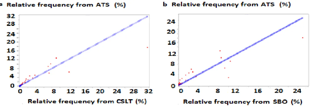
By comparing the activity-travel profiles derived from the call data with statistics that stem from traditional activity-travel surveys, the validation potential is demonstrated. In addition, a sensitivity analysis is carried out to assess how the results are affected by the different parameter settings defined in the profiling process.

Keywords activity-travel sequences, activity-based transportation models, travel surveys, mobile phone data.

1. Introduction

1.1. Activity-based transportation models

The main premise of activity-based micro-simulation transportation models is the treatment of travel behavior as a derived demand of activity participation. In this modeling paradigm, travel is analyzed through daily patterns of activity behavior related to and derived from the context of land-use and transportation network as well as personal characteristics such as social-economic background, lifestyles and needs of individuals (e.g. Bhat & Koppelman, 1999; Davidson et al., 2007; Fan & Khattak, 2012; Lemp et al., 2007; Wegener, 2013). All the above information, complemented with a training set of household travel surveys which document the full daily activity-travel sequences of a small sample of individuals during one or a few days, is analyzed and translated into heuristic decision making strategy rules. These rules represent the scheduling process of activities and travel by the individuals (e.g. Arentze & Timmermans, 2004; Bellemans et al., 2010). Once established they can be used as the probabilistic basis for a micro-simulation process, in which complete daily activity-travel sequences for each individual in the whole region are synthesized, using Monte Carlo simulation methods. The synthesized individual activity-travel sequences are then aggregated into origin-destination (OD) matrix, with each matrix element representing the number of trips between each pair of locations of the region. This matrix, after being assigned to a road network through traffic assignment algorithms, can subsequently serve as essential input for travel analysis in the region, such as travel demand forecasting, emission estimates and the evaluation of emerging effects caused by different transportation policy scenarios. Fig. 1 illustrates the entire process of a micro-simulation model.

3 Fig. 1. The entire process of an activity-based transportation model

1.2. Problem statement

Despite comprehension and advancement of the activity-based transportation modeling system, the lack of reliable data in sufficient size does not enable one to have a decent benchmark and evaluation criterion for the model output (e.g. Cools et al., 2010a; Cools et al., 2010b). Typically, for this purpose, one examines the results of the model both internally and externally at different stages of the simulation process, as indicated in Fig. 1 (e.g. Bellemans et al., 2010; Rasouli & Timmermans, 2013; Yagi & Mohammadian, 2010). The internal validation involves the comparison of the estimated results with expanded travel survey data which is not used in the training phase of the model but usually collected in the same survey period. In this validation, certain aggregated measures, e.g. the average travel distance and travel duration, derived from both the predicted sequences and the observed ones, are examined (e.g. Cherchi & Cirillo, 2010; Roorda et al., 2008). The sequence alignment method (SAM), which compares two sequences based on the composition and temporal ordering of the daily activities (Abbott & Forrest, 1986; Wilson, 1998), is also employed to assess the similarities between each of the observed sequences and its predicted counterpart (e.g. Sammour et al., 2012). However, the process involved in the development of the model, from initial data gathering to exploitation and validation of the first results, is lengthy and may take years, imposing a time lag between the data initially obtained and the data that is required for an objective and up-to-date validation measure. In addition to this time limitation, the high cost related to the surveys, makes it a challenge to collect samples in sufficient size, capable of providing a good representation of activity-travel behavior of a population. Moreover, travel surveys usually query information of only one or two days, in order to limit the negative effects associated with respondent burden. Consequently, this tends to obfuscate the less frequent activities, such as sports or telecommuting activities which are often carried out only once a week or once a month. These shortcomings have been well reported in the literature (e.g. Asakura & Hato, 2006; Cools et al., 2009).

In contrast to the internal validation, the external validation consists of an indirect evaluation of the model output at a later phase, i.e. traffic assignment stage (see Fig. 1). The estimated

Monte Carlo simulation for the whole population

OD matrix

Input: land use, transport network and survey data

Input: population socioeconomic data Model building

Output: Synthetic activity-travel sequences

Traffic assignment to road network

Internal validation: survey data

Activity-Travel sequence validation: mobile phone data

External validation: observed traffic count

Travel demand forecast, emission estimation and evaluation of transportation policy scenarios

OD-based validation: mobile phone data

4

traffic volumes at a number of predefined road segments are compared against information from external sources, such as traffic counts collected by inductive loop detectors which are deployed on the road segments.

However, the external validation process encompasses an aggregation step to compose the OD matrix as well as an assignment step to allocate the travel demand matrix to the road network. Valuable information may be lost in these two steps. Consequently, positive outcomes of the compared results might be artifacts of the validation process itself, and thus provide no real guarantee of the accuracy of the model. Moreover, when mismatches are found, there exists no clear procedure to trace back the causes, thus limiting the discovery of remedies to improve model construction. Nevertheless, despite such limitations, at the present, the indirect external evaluation is essentially the only option for model quality assessment in practice, as no well-established methods are found for operating closer to the model itself (e.g. Janssens et al., 2012). This is a problem that seriously hampers further model development and model application (e.g. Hartgen, 2013). Having useful and reliable benchmark and evaluation criteria for activity-based micro-simulation models has thus been a major concern.

1.3. Mobile phone data: a new data source for transportation modelling and validating

The wide deployment of mobile phone devices has created the opportunity to use the devices as a new data collection method to overcome the lack of reliable benchmark data (Jiang et al., 2013). Location data recorded from the mobile phone devices reflects up-to-date travel patterns on a significantly large sample of the population, making the data a natural candidate for the analysis of mobility phenomena (e.g. Do & Gatica-Pereza, 2013; Schneider et al., 2013). In addition, the data collection is a by-product of the mobile phone companies for billing and operational purposes that generates neither extra expenses nor respondent burden. The importance and added value of mobile phone data in the study of travel behavior and transportation modeling have been manifested by a variety of research efforts, ranging from the investigation of key dimensions of human travel, such as travel distance and time expenditure at different locations (e.g. González et al., 2008; Schneider et al., 2013; Song et al., 2010), to the discovery of mobility patterns and the construction of OD matrices (e.g. Bayir et al., 2009; Berlingerio et al., 2013; Calabrese et al., 2011; Huang et al., 2009), and to the examination of the status and efficiency of current transport systems (e.g. Angelakis et al., 2013; Hansapalangkul et al., 2007; Steenbruggen et al., 2013). Alongside these studies, mobile phone data has also been investigated to explore the possibilities of building model evaluation measures. Two recent research efforts can represent the state-of-art of such exploration. The first one (Shan et al., 2011) involves the use of mobile phone data of more than 0.3 million users collected in the metropolitan area of Lisbon, Portugal over a time period of an entire month. In their study, the two most frequent call cell towers for each of the users are first identified as the residential and employment locations. An OD matrix depicting the home-to-work commuting trips in the morning is then built, using the identified residential and employment locations as well as the call data. Based on a census survey, this matrix is subsequently scaled up to account for the total employed population of 1.3 million in the study area. The adjusted matrix is ultimately used to compare against the travel demand during the same morning period predicted by an integrated land use and transportation model developed in this region. In the entire activity-based modeling process, the above-described OD-based validation method can be positioned at the stage of OD matrix generation, as shown in Fig. 1.

Instead of an OD matrix, in the second research (Kopp et al., 2013), other mobility parameters, such as the number of frequently visited locations and the spatial extent of a person's daily mobility, are derived from mobile phone data collected in two separate regions,

5

namely a central region of Italy and a large area of Lausanne, Switzerland. As opposed to directly using the derived travel parameters to examine the simulation results from a transportation model, the research compares the parameter values derived from the mobile phone data with the results inferred from GPS data that is recorded in the same regions during the same periods and therefore portrays the same mobility phenomenon. The comparison results demonstrate the capability of the mobile phone data in reflecting real travel patterns of the population, thus suggesting its potentials of building an objective and more detailed evaluation standard for transportation models.

The two studies have provided deep insights into the characteristics of mobile phone data and illustrated its potentials for constructing an improved validation measure. In particular, the first research (Shan et al., 2011) has proposed a specific OD-based validation method and used a real transportation model to test this method’s applicability and viability. However, despite its advancement by incorporating mobile phone data into the model assessment, the OD-based method does not consider the sequential information which is imbedded in the activity-travel patterns. A detailed examination of the sequential dependencies of the daily activities from the simulated travel sequences is thus ignored in the validation process. It has been widely acknowledged that the choice of activities is dependent on the preceding activity engagement (e.g. Joh et al., 2007; Joh et al., 2008; Wilson, 2008), exemplified by the fact that, during one particular working day, it is highly probable that the combination of having breakfast, travel and working is observed together. On the contrary, if a sports activity is carried out in the morning, there is a small chance that it is performed again in the evening. The interdependencies of daily activities have been considered as a crucial factor in the activity-travel decision making process (e.g. Delafontaine et al., 2012; García-Díez et al., 2011; Saneinejad & Roorda, 2009; Shoval & Isaacson, 2007). The examination of how the predicted activity-travel sequences are consistent with the sequential constraints that are observed from the real travel patterns is thus important. In the existing validation methods for activity-based models, SAM has been employed to assess the similarities between each observed sequence and its predicted counterpart (e.g. Sammour et al., 2012), as previously described. But this evaluation is carried out against a small set of activity-travel sequences from travel surveys, thus subject to the shortcomings that are inherent to the traditional data collection method. A validation measure, which is based on massive mobile phone data while taking into account the sequential aspect of activity-travel behavior, has so far been lacking. 1.4. Research contributions

Extending the current research on the application of mobile phone data to travel behavior analysis and transportation modeling, and particularly addressing the above mentioned limitations in the development of reliable validation measures for activity-based models, our study proposes a new approach which is based on the phone data and which considers the sequential information hidden in activity-travel patterns. Specifically, the goal of this approach is to build a profile of workers’ activity-travel behavior, i.e. the relative frequency of each typical pattern which represents a certain class of activity-travel sequences, based on the mobile phone data. This profile can then be used to directly evaluate the sequences yielded from the simulation models, by comparing it against the frequencies of the corresponding pattern classes which are obtained from the simulated sequences (see Fig. 1). This comparison is carried out at the level of the generated activity-travel sequences, which enables the capability of detecting problems that are directly caused by the model itself and providing immediate feedback for the enhancement of the model.

Compared to existing validation measures, this approach offers the following advantages. (i) This method is built upon the observed current activity-travel behavior of a large proportion of population, thus providing a more representative and up-to-date validation

6

measure. (ii) Through a long period of mobile phone data records, inter- and intra- personal variations of travel behavior as well as weekday, weekend and seasonal deviations are captured. (iii) The use of mobile phone data generates no extra financial cost in terms of data collection, making it a cost-effective validation measure. (iv) This evaluation method directly examines the simulated travel sequences, and can thus offer immediate solutions to problems which are linked to the model system itself. (v) When this approach is compared with the recently developed OD-based validation method, the OD-based method examines the simulated sequences in terms of the distribution of the trips over different pairs of origin-destination locations; while the approach developed in this study focuses on the sequential aspect of the simulated sequences, and evaluates the distribution of the sequences over various classes of typical activity-travel patterns. In this new approach, the locations which are accessed by an individual on the same day are viewed and tackled as a whole, rather than an isolated participation in activities. Both measures assess the simulated sequences from different angles, thus providing a complementary means of benchmarking activity-based transportation models based on the mobile phone data.

The remainder of this paper is organized as follows. Section 2 describes the typical patterns which characterize workers’ activity-travel sequences. Section 3 introduces the mobile phone data and Section 4 details the construction process of location trajectories based on the data. The call location trajectories are then transformed into complete travel sequences by a method proposed in Section 5. Section 6 classifies both the call location trajectories and the travel sequences into the typical patterns which have been established in Section 2, and the profiles which describe the relative frequency of each pattern class are drawn. A case study is subsequently conducted in Section 7, and a comparison of the results against the outcomes of real travel surveys is carried out in Section 8. An in-depth analysis on the sensitivity of this approach is further performed in Section 9. Finally, Section 10 ends this paper with major conclusions and discussions for future research.

2. Activity-travel sequence classification

Individuals make choices about the different activities being pursued, and travel may be required to participate in these activities. Traditionally, all activities performed at home are considered as home activities; while the remaining ones conducted outside home are categorized into mandatory activities (e.g. working or studying) and non-mandatory activities that include maintenance activities (e.g. shopping, banking or visiting doctors) and discretionary activities (e.g. social visit, sports or going to restaurant) (e.g. Arentze & Timmermans, 2004; Bradley & Vovsha, 2005). The home, mandatory and non-mandatory activities are represented as ‘H’, ‘W’ and ‘O’, respectively.

The sequence of activities and travel that a person undertakes during a day is referred as the individual’s travel sequence for that day. A critical difference is imbedded in activity-travel sequences between workers and non-workers; the sequences of workers mostly rely on the regularity and fixity of the work activity. In contrast, no such obvious periodicity is present in the case of non-workers. This motivates the development of separate representations for these two types of individuals’ behavior. In this study, only the activity-travel behavior of workers is analyzed, and the representation of their daily sequences described in the research by Spissu et al. (2009) is adopted. In this representation (see Fig. 2), an activity-travel sequence is divided into four different parts, including: (i) before-work sub-sequences which represent the activities and travel undertaken before leaving home to work (as indicated in arrows ‘a’), e.g. HOH; (ii) commute sub-sequences which account for the activities and travel pursued during the home-to-work and work-to-home commutes (in arrows ‘b’ and ‘d’), e.g. HOW or WOH; (iii) work-based sub-sequences which accommodate

7

all activities and travel undertaken from work (in arrows ‘c’), e.g. WOW; (iv) after-work sub-sequence which comprises the activities and travel engaged after arriving home from work (in arrows ‘e’), e.g. HOH.

Fig. 2. The representation of workers’ activity-travel sequences

Note: Each ‘rectangular’ indicates the home or work location, while the ‘diamond’ represents a non-mandatory activity location. Each ‘arrow’ from a home, work or non-mandatory activity location to the other location represents the related travel, and the ‘arrow’ from a non-mandatory activity location to itself indicates the chain of consecutive visits to different non-mandatory activity locations.

According to the above characterization, a home-based-tour, which is defined as a chain of locations (trips) that start and end at home and accommodates at most two work location visits, can be classified into the following patterns: HWH, HOWH, HWOH, HWOWH, HOWOH, HOWOWH, HWOWOH, HOWOWOH, where each H or W stands for a home or work location while each O represents one or a chain of visits to several non-mandatory activity locations. The days when an individual does not go to work, can be characterized with 2 additional patterns, namely H and HOH. In total, 10 classes are formed to identify each based-tour in a worker’s daily activity-travel sequence, and they are defined as home-based-tour-classification.

Every pair of the above pattern classes (excluding H) is then merged, leading to 81 combinations of daily sequences which contain 2 home-based-tours. For instance, the combination of HWH and HOWH results in the sequence HWHOWH. The daily sequences that represent only a single home-based-tour with maximum two work location visits, e.g. HWOWH, are also clustered, according to the home-based-tour-classification. Finally, the remaining sequences which contain more than 2 home-based-tours (e.g. HWHWHWH) or which have more than 2 work activity locations in a home-based-tour (e.g. HWOWOWH), are each assigned into one additional category. Thus, all the above classification leads to a total of 93 patterns which underlie workers’ activity-travel behavior, and are denominated as the workers’ daily-sequence-classification. Given a group of individuals, their activity-travel sequences can be attributed to the corresponding pattern classes. The relative frequency of each of the pattern classes over the total number of activity-travel sequences forms the profile of activity-travel behavior among these people.

e e e d d d d c c b b b b a a O O O

Home(H) Work(W) Home(H)

O

a c

8

3. Mobile phone data description

The mobile phone dataset consists of full mobile communication patterns of around 5 million users in Ivory Coast over a period of 5 months between December 1, 2011 and April 28, 2012 (Blondel et al., 2012). The dataset contains the location and time when each user conducts a call activity, including initiating or receiving a voice call or message, enabling us to reconstruct the user’s time-resolved call location trajectories. The locations are represented with the identifications of base stations (cells) in a GSM network; the radius of each of the stations ranges from a few hundred meters in metropolitan to a few thousand in rural areas, controlling our uncertainty about the user’s precise location. Despite the low accuracy of users’ exact locations, the massive mobile phone data represents a significant percentage (i.e. 25%) of this country’s population, providing a valuable source and opportunity for the analysis on human travel behavior and for drawing relevant inferences that can be statistically sound and representative.

In order to address privacy concerns, the original dataset has been split into consecutive two-week periods. In each period, 50,000 of all the users are randomly selected and assigned to anonymized identifiers. New random identifiers are chosen for re-sampled users in different time periods. The data process results in totally 10 randomly sampled datasets, each of which contains communication records of 50,000 users over two weeks. One of the datasets is selected for this study. Table 1 illustrates typical call records of an individual identified as User2 on Monday, December 12th, 2011.

Table 1. The typical call data of an individuala

Time 11:57:00 13:40:00 16:59:00 17:43:00 21:28:00

Antenna_id 898 1020 972 926 926

a _{The ‘time’ represents the moment (i.e. the hour, minute and second) when this user was connecting to the} GSM network and the ‘Antenna_id’ as the cell area where he/she is located.

4. Construction of call stop location trajectories

A raw-location-trajectory from a mobile phone user during a day is defined as a series of locations where the user makes calls when traveling or doing activities, as the day unfolds. It can be formulated as a sequence of l1 -> l2 -> … -> ln, where n is the length of the sequence, i.e. the total number of locations that the user has travelled to when making calls that day, and li (1 ≤ i ≤ n) is the identification of the locations, e.g. cell IDs in this study. At each li, there could be multiple calls, referred as call-frequency, denoted as ki (ki ≥ 1); the time for each of the calls is as T(li,1), T(li,2), …, T(li,ki), respectively. The time interval between the first and the last call time in the set of consecutive calls, i.e. T(li,ki) – T(li,1), is defined as call-location-duration. Accommodating the time signatures of the multiple calls, a raw-location-trajectory can be represented as l1(T(l1,1),T(l1,2),…,T(l1,k1)) -> … -> ln(T(ln,1),T(ln,2),…,T(ln,kn)), simplified as l1(T(1),T(2),…T(k1)) -> … -> ln(T(1),T(2),…,T(kn)). Given the above raw-location-trajectories constructed from the mobile phone data, the home and work locations are first predicted. This is followed by the identification of stop locations where activities are being carried out.

4.1. Prediction of home and work locations

Various methods have been proposed to derive home and work locations from mobile phone data, mainly based on the visited frequency of a location during a particular time period (e.g. Becker et al., 2011; Calabrese et al., 2011). However, different time windows have been specified in these methods, depending on the context of the study area. In this study, a similar approach is adopted, but the time windows are empirically estimated from the mobile phone

9

data as follows. The time period when call activities start to increase considerably in the morning during weekdays is chosen as the work start time, denoted as work-start-time. Similarly, the moment when the second peak of call activities start to appear in late afternoon is considered as the work end time, referred as work-end-time. Around this time, it is assumed that people start to communicate for off-work activity engagement.

Based on these two temporal points, a location is defined as the home location if it is the most frequent stop throughout the weekend period as well as during the night-time interval on weekdays between work-end-time and work-start-time. On the contrary, a location is considered as a work place if it satisfies the following criteria. (i) It is the most common place for call activities in the perceived work period between work-start-time and work-end-time on weekdays. (ii) It is not identical to the previously identified home location for the user. (iii) The calls at the location are not limited in only one day, they should occur at least 2 days a week.

With the identification criteria, we assume that people have only one home location and at most one work location. The additional locations, which are occasionally accessed for home or work activities, are regarded as a stop for non-mandatory activities. In addition, only individuals, who work at locations different from their home locations and who work at least two days per week, are included for the analysis of workers’ travel behavior.

4.2. Identification of stop locations

After the identification of the distinct home and work locations for each worker, the remaining locations in the raw-location-trajectories are either stop-locations where people pursue non-mandatory activities or non-stop-locations. Each of these non-stop-locations can be further classified into either a trip-location where the user is traveling, or a false-location that is wrongly documented due to location update errors. The location update errors normally occur when call traffic is busy in the user’s real location area, and consequently this location is shifted to less crowded cells for short time periods, causing location area updates, without the users’ actual moving (e.g. Calabrese et al., 2011; Schlaich et al., 2010).

In addition, for the identified home or work locations, some occurrences of the locations could also be caused by non-stop reasons, e.g., people travelling in the same area as their home locations when making calls. Therefore, each location occurrence in the raw-location-trajectories will be classified into stop-locations and non-stop ones, regardless its activity type.

The scenarios, where the two types of non-stop-locations discussed above could occur, can be illustrated with the call records of two typical users. The trajectory from the first user, identified as User265, is l1(17:06,17:43) -> l2(17:51) -> l3(17:56,19:41) -> l4(21:55), where 4 locations are observed, with the call-location-duration as 37, 0, 105 and 0 min respectively. From this trajectory, a distinction needs to be made to identify stop visits from possible trip visits at each of these locations. The trajectory of the second user known as User72 is l1(13:21,20:11) -> l2(22:00) -> l3(22:02) -> l4(22:05) -> l2(22:07,23:12). This user has 5 location updates, with the call-location-duration as 410, 0, 0, 0 and 65 min respectively. It should be noted that the time interval between the first and second visit of location l2 is only 7 min. Although there is a possibility that this user may have travelled at a high speed during this period, the temporary interruption of l2 by the extra locations l3 and l4 in such a short interval is most likely resulted from the location update errors. Consequently, locations l3 and l4 are falsely connected to the user’s mobile phone at 22:02 pm and 22:05 pm although he/she had been actually remaining at location l2 _{during this period.}

10

4.2.1. Identification process

Schlaich et al. (2010) have proposed a method to distinguish a stop-location from a non-stop one. In their approach, the interval between the first logins of two adjacent locations li and li+1, i.e. T(li+1,1) – T(li,1), is examined. If this interval is longer than a time limit, e.g. 60 min in their experiment, li is considered as a stop-location. However, this method is likely to overlook stop-locations where calls are made just before the departure of the locations. In this situation, the time interval can be very short, despite the possibility that users may spend a considerable time period at the locations. This can be further illustrated with the case of User265. The interval between the two first time signatures of locations l1 _{and l}2 is 45 min, shorter than this 60-min limit, suggesting that location l1 would be for trip purposes. This may be true if this individual has made a long trip of at least 37 min within l1and made calls at the start and end of this travel. However, if this individual has stayed there doing activities for a long time, e.g. a few hours, and he/she made calls later in this sojourn period, location l1 is then misclassified by the existing method.

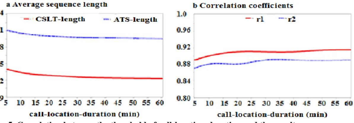
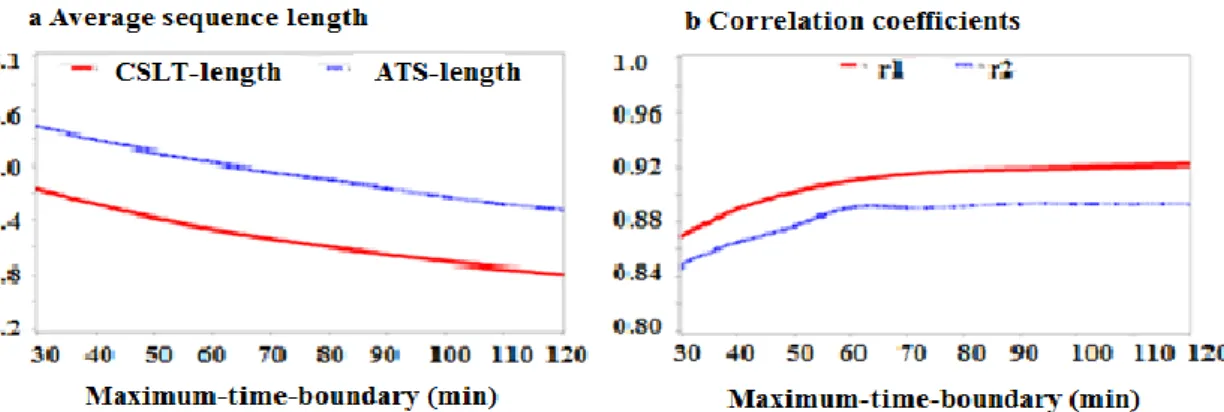
In order to identify all the possible stop-locations, we propose a new approach consisting of the following steps. (i) For each location li, the call-location-duration is first examined. If it is longer than a certain time limit, denoted as Tcall-location-duration, this location is considered as a stop-location. (ii) Otherwise, if the condition does not hold (e.g. only a single call made at li), and if the location occurs in the middle of a daily sequence of n, i.e. 1 < i < n, a second parameter, namely maximum-time-boundary, defined as the time interval between the last call time at li’s previous location and the first call time of its next location, i.e. T(li+1,1) – T(li-1,k i-1), is computed. If this time period is longer than a threshold value, defined as T maximum-time-boundary, li is perceived as a stop visit. (iii) When li is in the first or last position of a trajectory and the call-location-duration is shorter than Tcall-location-duration, there is no sufficient information to estimate maximum-time-boundary for this visit. Thus, all the distinct locations, where the user has stayed at least once for conducting an activity over the entire survey period, are collected. These locations are considered as potential stop locations that are on the user’s daily activity agenda and that are visited either routinely or once in a while. If li is one of these locations, it is assumed to be a stop for activity purposes. In contrast, if li is the place where the individual has not been observed doing activities, it is then considered as a passing-by place or being recorded as a localization error and therefore removed.

Based on the above described identification process, if a duration of 30 and 60 min are used for Tcall-location-duration and Tmaximum-time-boundary respectively, as set up in our experiment, the obtained trajectory of stop locations for User265 and User72 are l1 -> l3 -> l4 and l1 -> l2 respectively. In comparison, using the existing method which only considers the first temporal logins of two consecutive locations (Schlaich et al., 2010), only one single location would be derived for each of these users, which is l3 for User265 and l1 for User72.

After the removal of locations that are either trips or stemming from localization errors, all the remaining locations from a raw-location-trajectory are regarded as stops and stored into a stop-location-trajectory. Each location li in these stop-location-trajectories is complemented with its function, categorized into home, work and non-mandatory activities, denoted as activity(li). Travel is implicit in between each two consecutive locations of these sequences.

11

5. Transformation of call stop location trajectories into actual travel sequences

The considered mobile phone dataset is event driven, in which location measurements are only available when the devices make GSM network connections. Consequently, users’ call behavior can affect the possibility of capturing a larger or smaller number of trips and/or activity locations. In general, the more active a user is in communicating electronically with others, the better his/her activity-travel behavior is revealed by his/her call records. The call locations can be seen as the observed behavior at certain temporal sampling moments during a day, and the characteristics of the real travel behavior must be deduced. A transformation therefore should be made from the previously derived stop-location-trajectories into the sequences that mirror the real picture of people’s activity-travel behavior.

During this transformation, we first derive for each user the actual activity duration as well as the call rate at each minute. These two variables are then translated into the call probability at each location, which describes how likely the individual makes at least one call when he/she visits the location and which thus indicates to what extent his/her call records reveal his/her actual movement. Next, given a real daily activity-travel sequence, various stop-location-trajectories could be possibly observed from the call data. The probability, under which a certain stop-location-trajectory is generated from the original travel sequence, is calculated based on the call probabilities at the actually visited locations. Finally, given the observed frequencies of the stop-location-trajectories derived from the call data, a linear equation is built and the frequencies of the original travel sequences are inferred.

5.1. Call rate and actual location duration

Call-intervene for a user measures the time interval between each two calls, and it is calculated as the ratio between the total number of calls each day, denoted as total-number-calls, and the time span of the day (measured in min), denoted as time-span, as follows:

day) (user calls number total span(day) time user ervene call day day , ) ( int       

Based on the call-intervene, the call rate defined as CallRate, which describes the probability that a user makes calls each minute, can be calculated as follows:

) ( int 1 ) ( user ervene call user CallRate  

Let the variable actual-location-duration(user,li) represent the actual activity duration (in min) which a user spends at location li. Given that this information is unknown from the phone data, we thus turn to activity-travel surveys to obtain the real behavioral data. This duration variable is approximated by the average duration over all respondents in a survey across all locations with the same activity purposes, defined as average-location-duration(activity(li)).

5.2. Call probability at a location

Given a user’s call rate and the duration that the individual has actual spent at li, the probability of making at least a call during the entire period of the visit to the location, defined as CallP(user,li), can be estimated in the following manner. The location duration is first divided into a number of equal-interval episodes, and each of the episodes can be regarded as an experiment. The length of the episodes, referred as EpisodeL, can be estimated,

12

e.g. by the average time that people spend on the phone each time when they are in the connection of the GSM network, e.g. 2 min for voice calls and a few seconds for the messages. Under the assumption that the user makes calls (including both initiating and receiving voice calls and messages) independently in each episode, and that the probability of making calls across different episodes at the location is identical, CallP(user,li) can then be modeled as the binomial distribution. The actual location duration delimits the total number of episodes, i.e. the number of independent experiments. While the call rate provides the probability of success for each experiment result, that is the probability of making a call in each episode. This leads to the final estimation of the probability CallP(user,li) as the probability of having at least one success (making at least one call) over the total number of experiments, in this case, over the total location duration.

In this study, the previously derived two variables CallRate and average-location-duration are used as the approximation of the call rate for a user and the duration for a location with a particular activity purpose, respectively. The probability CallP(user,li) is then obtained as follows: )} ( 1 { 1 ) ( , , / ) ( user CallRate EpisodeL ) l activity CallP(user ) l user CallP( EpisodeL ) ctivity duration(a location average l i i i       

5.3. Sequence conversion probability

After the probabilities of making calls at a location of home, work or non-mandatory activities for a user are known, the likelihood that a call location trajectory is generated from an actual activity-travel sequence can be derived. In addition to the assumption that users make calls independently in each episode during a location visit, we also hypothesize that they make calls independently across each location visit. Let the sequence l1 -> l2 -> … -> ln represent the actual-travel-sequence for a user. Based on the previously derived probabilities CallP(user,li), the likelihood of various stop-location-trajectories that could be observed from the actual-travel-sequence, defined as the conversion probability ConversionP, can be calculated as shown below. The probability that the original complete travel sequence can be revealed by the call records is:

1 2 2

1

ConversionP( , , )

ConversionP( , ... n, ... n) n ( , i).

i

user actual travel sequence stop location trajectory

user l l l l l l callP user l



   

       

While the probability that only a part of the travel sequence is observed, is

























callP user l callP user l

                 







and where, we assume that no phone communications have been made during the visits to locations from xi to xj (i ≤ j).

The above described sequence conversion process can be illustrated by the call data of User121 in our dataset. The probabilities to make at least one call at the locations of home, work and non-mandatory activities for this user are 0.805, 0.903 and 0.424, respectively. Suppose the sequence of HWOH represents the actual activity-travel behavior of this

13

individual on a certain day, there could be a total of 15 various call location traces generated by this travel sequence, and the sum of the corresponding conversion probabilities is 1. For instance, the possibility to emanate the call trajectory of HWH is ConversionP(user121, HWOH, HWH) = 0.34.

5.4. Derivation of activity-travel sequences

Based on the previously obtained conversion probabilities and the frequencies of the observed call location trajectories, the occurrences of original activity-travel sequences can be ultimately derived. Suppose that m different stop-location-trajectories s1,s2,…,sm are constructed from a user’s call records with the observed frequencies as y1,y2,…,yk respectively, and that they are sorted by the length of these sequences, i.e. length(s1) ≥ length(s2) ≥ … ≥ length(sm). The original occurrences of the corresponding travel sequences for the user, denoted as x1,x2,…,xk, can be estimated by the following linear equations; to simplify, the parameter of user in the function ConversionP()is omitted here:

            1 1 1 1 1 1 2 2 2 2 2 1 1 2 2 , , , , _k , _k ... _{k k}, _{k k} x ConversionP s s y x ConversionP s s x ConversionP s s y

x ConversionP s s x ConversionP s s x ConversionP s s y

                    (1)

An additional constraint is added to the unknown variables x1,x2,…,xk, in order to ensure that the total number of the derived travel sequences is equal to that of the observed call trajectories, i.e. 1 1 k k i i i i x y   





1 1 1 k k k i i i i x y x    





formation of formula (2) as follows:

                1 1 1 1 1 1 1 2 2 1 1 1 1 1 1 1 1 1 , , , ... , , , ... , , k k k k k k k k k k k k k k k x ConversionP s s y

x ConversionP s s x ConversionP s s x ConversionP s s y

x ConversionP s s ConversionP s s x ConversionP s s ConversionP s s

y Conver                  _  _  _  _     1 , k k k i i sionP s s y             



Formula (2) is a model with k equations and k–1 unknown variables. To find the optimal solution, we use Linear Least Square Methods which are a standard approach to find the solution to a set of unknown factors from a model that has more equations than the unknowns (Chen & Plemmons, 2009; Van de Geer, 2000). This approach searches for the answer by minimizing the sum of the squares of errors (or residuals) made in the results of every single equation. A residual is the difference between an observed value and the fitted value provided by the estimated model. As well as minimizing the total sum of squared residuals, the obtained results also maximize the likelihood of the observed values, i.e. the frequencies of the observed call location trajectories in this study.

Specifically, to solve the equations in formula (2), we assume the least square estimators are:

1 2 1

ˆ ˆ, , ,ˆ_k ;

x x x _

14 ] ) , ( P Conversion [ )] , ( P Conversion ) , ( P Conversion [ ˆ )]... , ( P Conversion ) , ( P Conversion [ ˆ ... ) , ( P Conversion ˆ 1 1 1 1 1 1 1 1 1 1                k i i k k k k k k k k k k k k y s s y s s s s x s s s s x residual y s s x residual

The total sum of the squared residuals, denoted as Sum, can be obtained as

   k i residuali Sum 1 2 ) ( .

The minimum of Sum is then found by setting its partial derivatives to zero, which is

.

1

,...

1

,

0

ˆ











k

i

x

Sum

The above models have the equal number of (i.e., k-1) equations and unknown variables, thus leading to the final

resolution of the estimators xˆ1,xˆ2,...xˆk1_{, as well as of the estimator}

x

ˆ

as









ˆ

ˆ

y

x

x

In the case of User121, five different stop-location-trajectories are revealed by his/her call records over a total of 10 days, including HWOH, WH, OH, W and H, with the occurrences as 1, 3, 2, 1 and 3 respectively. The original frequencies of these sequences, i.e. x1-x5, are

estimated based on the above described methods as

14 . 0 ˆ , 07 . 0 ˆ , 89 . 4 ˆ , 74 . 3 ˆ , 17 . 1 ˆ1 x2 x3 x4 x5

x , with the total sum of the squared residuals

between the modeled frequencies and the real observed values is Sum = 0.74.

It can be noted that during the entire procedure of seeking the optimal solution, we assume that the original travel sequences could only occur within the space of observed call location trajectories, i.e. Space = {s1,s2,…,sm}. In theory, however, there could be a chance that an observed call location trajectory is generated by many other potential travel sequences, rendering the solution space infinite. The definition of the search space of Space can be explained as follows. (i) Based on the well-established findings that human activity-travel behavior exhibits a high degree of spatial and temporal regularities as well as sequential ordering (e.g. Joh et al., 2008; Shoval & Isaacson, 2007; Wilson, 2008), a limited variety of real travel sequences for an individual can be assumed during a certain time scale. (ii) For a possible actual travel sequence, e.g. sp, which is not in the observed Space, the optimal estimator of this sequence’s actual occurrence xp would be a value less than or equal to zero, due to the fact that the observed frequency of this sequence in its intact form is zero. This can be further demonstrated as follows. For User121, if the considered travel sequence sp is longer than any trajectory in the Space of this user, i.e. length(sp) ≥ length(s1), assume sp = HWOWH, we obtain the equation as xp × ConversionP(HWOWH,HWOWH) = 0. From this equation, we have the optimal solution as _{xˆ 0}

p . Similarly, if the length of sp is shorter than certain observed trajectories in the Space, e.g. sp = HWO, we have the equation of x1 × ConversionP(HWOH,HWO) + xp × ConversionP(HWO,HWO) = 0, from which a value of

0 ˆ 

xp would be preferable. Based on the above two considerations, the optimal solution of

the frequencies of original travel sequences would most likely found within the space of Space.

15

6. Classification

All the obtained stop-location-trajectories constructed directly from the call records as well as the actual-travel-sequences that undergo a transformation process, are subsequently classified according to the previously established home-based-tour-classification and daily-sequence-classification, respectively. During this daily-sequence-classification, a home location H is added at the beginning and the end of a sequence if it is absent from this sequence, based on the assumption that each individual starts and ends a day at home. For each of these two types of sequences, two corresponding profiles are obtained and they are stored into matrices, namely home-based-tour-profile and daily-sequence-profile.

The Pearson correlation coefficient r is used to measure the relation between the corresponding profile matrices built from different sets of sequences. It reveals the strength of linear relationship between two matrices; the closer the value is to 1, the stronger the relationship is. The coefficient is computed as follows.

. 1 , ) ( , ) ( , , 1 1 2 1 2 1 1                                 d S B B S A A r d B B S d A A S d B B d A A B i d i A i d i i B d i i A d i i d i i . 1 , ) ( , ) ( , , 1 1 2 1 2 1 1                                 d S B B S A A r d B B S d A A S d B B d A A B i d i A i d i i B d i i A d i i d i i

Where, Ai and Bj represent the matrix elements of the two concerned matrices A and B, respectively, with d as the total number of the matrix elements.

7. Case study

In this section, adopting the proposed profiling approach and using the mobile phone data described in Section 3, we carry out an experiment. In this process, a set of stop-location-trajectories are first constructed, followed by the translation of the stop-location-trajectories into actual-travel-sequences. Each step of this process is highlighted with the examination of some particular parameters.

7.1. Construction of stop-location-trajectories 7.1.1. Work-start-time and work-end-time

Fig. 3 describes the distribution of the frequencies of calls made in each hour of the weekdays, showing that from 9am in the morning, calls reach to their peak level; while from 18pm in the late afternoon, a second climax of call activities starts to occur. These two temporal points are chosen as the work-start-time and work-end-time, respectively.

16 Fig. 3. The distribution of the time of calls

Based on the pre-defined criteria for home and work location identification, 49436 (98.9% of the total) users have their home locations discovered. The remaining 1.1% are those who made no calls at weekend or in the night period from 18pm to 9am across the two surveyed weeks. As a result, their homes cannot be spotted by these rules. Meanwhile, 9,458 users (18.9% of the total) are screened out as employed people, if they work between 9am and 18pm at least two weekdays per week. By contrast, those who work at night shifts or at weekends, who work less than two days a week, or who make few calls at work, are left out. For those who have both predicted home and work locations, we further remove nearly 15% of the individuals who have unknown cell IDs for the identified home or work locations due to technical reasons that occur in the mobile phone data collection process. This results in a final dataset of 8,027 workers who represent 16% of the total users in the selected dataset. All the call records of these individuals during weekdays are extracted, and the consecutive calls made at a same location are aggregated. This leads to 69,578 raw-location-trajectories constructed for further analysis.

7.1.2. Tcall-location-duration and Tmaximum-time-boundary

For each location in the above obtained raw-location-trajectories, a distinction must be made between stop-locations and non-stop ones which include trip- and false-locations. Two parameters characterize this identification process. The first one, Tcall-location-duration, defines the minimum time interval at a location, above which the location is considered as a possible stop. The other parameter, Tmaximum-time-boundary, estimates the total time that is required to travel from the previous cell to the current one and from the current one to the next cell. In addition, it should also be able to detect location update errors which usually occur in a short time interval.

In this experiment, Tcall-location-duration and Tmaximum-time-boundary are set as 30 min and 60 min respectively. Under these thresholds, 40.3% of all locations from the raw-location-trajectories are removed; the remaining locations in these sequences form the set of stop-location-trajectories. The average length of these trajectories is 3.3. In comparison, using the existing method which defines as a stop location if the interval between the first login of the location and that of its next location is longer than 60 min (Schlaich et al., 2010), 67.6% of all the call locations are dismissed, with the average length of the retained sequences as 2.33.

17

7.2. Transformation from stop-location-trajectories into actual-travel-sequences 7.2.1. Call-intervene and CallRate

For each user, all the calls made over the two survey weeks are counted, and the intervene and CallRate are computed based on the formulas in Section 5.1. The average call-intervene over all the identified workers is 192 min for a full day of 24 h. However, as demonstrated in Fig. 3, the occurrences of calls are not equally distributed, more calls are observed during the day than at night, the inclusion of the night period would bias the real call intervene time during the daytime period. In this study, only the period of 6am-12pm is thus taken into account as the time-span of a day. This reduces the average call intervene to 137 min; accordingly, the average call rate is 0.0073.

In the study reported by Calabrese et al. (2011), a 260 min of call intervene for an entire day is derived. The difference between the call intervene reported in this study and the one estimated by Calabrese et al. could be caused by the following factors. (i) Only workers are considered in our study. (ii) The mobile phone data in this experiment is more recent than the data used in the existing study. (iii) People could make more calls in Ivory Coast than in Massachusetts in the United States where the existing study is performed.

7.2.2. Average-location-duration

This variable value is approximated by the activity-travel survey conducted in Belgium which will be described in Section 8.2. From this survey, the average-location-durations are 222, 317 and 75 min for home, work and non-mandatory activities, respectively.

7.2.3. Episode length

This variable specifies the time window by which the location duration is split into a number of episodes, i.e. experiments. The length of this window is decided such that the call behavior of users in one episode should be independent of that in the next episode. To obtain such an episode length, the average voice call duration of users is considered, which is derived from an additional dataset that records the total number of voice calls as well as the total duration for these calls each hour between each two cells in the GSM network in Ivory Coast, over the 5-month data collection period. The resultant average call duration is 1.92 min, a 2-min interval is thus taken as the estimation of this episode length.

Based on all the above parameter settings, the call probabilities at a location of home, work and non-mandatory activities for a user are respectively derived; the average call probabilities over all the individuals for the three types of activity locations are 0.81, 0.88 and 0.41, respectively. These obtained probabilities of each user, combined with the observed frequencies of the stop-location-trajectories for the individual, lead to the prediction of the number of the actual-travel-sequences, using the method described in Sections 5.3 and 5.4. 8. Comparison of the results derived from mobile phone data with real activity-travel surveys

To illustrate the practical ability of our approach to really serve as a benchmark, we compare the results derived from the mobile phone data with the statistics drawn from real activity-travel surveys. Unfortunately, no official activity-activity-travel surveys have been documented in Ivory Coast. Therefore, data stemming from other countries, including South Africa and Belgium, has been adopted for this purpose. The authors acknowledge that the real travel behavior in Ivory Coast most likely is considerably different from the one reported in South Africa and Belgium. Consequently, the illustration serves to underline the applicability of the approach, not to infer the travel behavioral relationships in this particular case. The

18

comparison is carried out in two aspects, including the aspect of individual locations, e.g. the average number of locations visited each day, and the sequential aspect of the activity locations, e.g. the home-based-tour-profile and the daily-sequence-profile.

8.1. The travel survey in South Africa

The South Africa National Household Travel Survey (NHTS) was the first national survey of travel habits of individuals and households, aimed at making significant improvements in public transport services. The survey was based on a representative sample of 50,000 households throughout South Africa and undertaken between May and June in 2003 (Department of transport, 2003)

The information recorded by the survey includes the travel time to various public transport modes, e.g. trains and buses, as well as to activity locations, e.g. shops and post offices. The number of trips and the purposes for these trips are also documented for each individual on a typical weekday. The survey results reveal that the majority of the respondents can access to most of the activity services within half an hour (i.e. the travel time), and the average number of activity locations visited by a worker on a weekday is estimated between 3.46 and 4.06.

8.2. The travel survey in Belgium

Despite the relative geographic proximity between South Africa and Ivory Coast, the information on the NHTS survey is nevertheless limited. Particularly, the detailed travel patterns for each individual are not accessible for us. This necessitates the use of a second survey that provides activity-travel sequences on entire days and will be used as a reference for the illustration of the derived profiles.

The survey, namely SBO, stems from a large scale Strategic Basic Research Project on transportation modeling and simulation, and it was conducted on 2500 households between 2006 and 2007 in Belgium. In this survey, the respondents recorded trip information during the course of one week, such as trip start time and end time, purpose of the trip (e.g. activity type), and trip origin and destination (e.g. activity location). The average travel time is 24 min, comparable to the 30 min for a typical travel in South Africa.

In the SBO survey, activity locations are represented with statistical sectors, each of which ranges from a few hundred meters to a few thousands in radius, similar to the spatial granularity level of cell locations in GSM network. Table 2 illustrates a typical diary of respondent identified as ‘HH4123GL10089’. Only the variables that are relevant for the current study are presented in this table; a more detailed variable list and elaboration on the survey can be found in (Cools et al., 2009).

Table 2. Activity-travel diary data

Respondent ID Date Trip Start Time Trip End Time Trip Origin Trip Destination Trip Purpose HH4123GL10089 09/05/2006 07:45:00 08:00:00 34337 34345 Work HH4123GL10089 09/05/2006 17:00:00 17:15:00 34345 34349 Shopping (non-mandatory) HH4123GL10089 09/05/2006 17:40:00 18:05:00 34349 34337 Home

From the dataset, the diaries from 372 individuals who work at least two days a week are extracted. Note that only the activity-travel sequences recorded on weekdays are extracted. Activity duration at the destination of a trip is estimated as the time interval between the end time of the trip and the start time of its next trip, if the activity is not the first and the last one of a day. Otherwise, the duration is approximated in combination with the typical time for getting up in the morning and going to sleep in the evening in Belgium, which are estimated as 6am and 12pm, respectively (Hannes et al., 2012). An assumption that respondents start

19

and end a day at home, is also made, when the activity duration is calculated. Based on the above process, the duration of each activity for each individual on each weekday is computed. For instance, the previously demonstrated respondent has a daily activity sequence of HWOH, with the activity duration as 105, 540, 25 and 355 in min, respectively. All the obtained activity durations are averaged per activity type over all the individuals, and stored in the variable average-location-duration(activity), which has been previously used in the experiment to derive the actual-travel-sequences.

8.3. Statistics on the average length of sequences

Table 3 summarizes the statistics on the average number of locations visited each day, i.e. the average length of sequences, derived from the sequences of raw-location-trajectories, stop-location-trajectories and actual-travel-sequences which have been previously built based on the mobile phone data. The results drawn from both the NHTS and SBO surveys are also presented alongside as a comparison.

Table 3. Statistics on the average length of sequencesa

Sequences RLT CSLT ATS NHTS SBO

Average length of sequences 5.69 3.30 4.02 3.46-4.06 3.96

a_{The columns from left to right represent the raw-location-trajectories (RLT), call stop-location-trajectories} (CSLT), actual-travel-sequences (ATS), NHTS and SBO surveys, respectively. The same abbreviation for each type of sequences will be used throughout the remaining tables and figures in this paper.

From Table 3, it was observed that the average length of sequences first drops from initial 5.69 for the raw-location-trajectories to 3.3 for the stop-location-trajectories, and then rises again to 4.02 for the estimated travel sequences which is the closest to the number observed in both NHTS and SBO surveys. In addition, the differences in this variable value imply the importance of the process from the identification of stop locations to the inference of complete travel sequences proposed by our approach, when analyzing activity-travel behavior based on the mobile phone data.

8.4. Home-based-tour-profile

Table 4 shows the relative frequency of each pattern class in the home-based-tour-classification, obtained from the stop-location-trajectories, the actual-travel-sequences and the SBO diaries, respectively. The differences in the frequencies of each pair of corresponding pattern classes are also listed.

Table 4. Home-based-tour-profile (%)a

Typical patterns CSLT ATS SBO ATS - CSLT CSLT - SBO ATS - SBO

H 9.0 4.4 6.4 -4.6 2.6 -2.0 HWH 50.3 39.1 42.9 -11.2 7.4 -3.8 HOH 18.0 26.3 32.5 8.3 -14.5 -6.2 HOWH 5.1 6.7 3.1 1.6 2.0 3.6 HWOH 8.2 10.3 10.8 2.1 -2.6 -0.5 HWOWH 3.4 3.8 1.6 0.4 1.8 2.2 HOWOH 2.5 4.1 1.9 1.6 0.6 2.2 HOWOWH 0.7 1.0 0.2 0.3 0.5 0.8 HWOWOH 1.4 2.1 0.5 0.7 0.9 1.6 HOWOWOH 0.5 0.8 0.1 0.3 0.4 0.7

More than 2 work activities

1.0 1.3 0.2 0.3 0.8 1.1

a _{The columns from left to right represent the typical patterns, the frequency of each pattern class relative to the} total number of sequences within each type of CSLT, ATS and SBO, and the pairwise differences in the frequencies for each pattern among these three types of sequences, respectively.