Calculation of the scattering coefficient of a sine-shaped surface by using the BEM method

CALCULATION OF THE SCATTERING COEFFICIENT OF A

SINE-SHAPED SURFACE BY USING THE 3D BEM

METHOD

L De Geetere K.U.Leuven, Laboratory of Building Physics and Laboratory of Acoustics, Belgium JJ Embrechts University of Liege, Dept. of Electrical Engineering and Computer Science, Belgium G Vermeir K.U.Leuven, Laboratory of Building Physics and Laboratory of Acoustics, Belgium

1

ABSTRACT

Scattering or diffusion coefficients may be measured or calculated from polar reflected pressure diagrams1,2. It is common practice to evaluate these polar diagrams in the far field because the relative pressure magnitude as a function of reflection angle is independent of the distance to the reflector and so the scattering or diffusion coefficient becomes independent of the receiver distance. This makes it easier to compare different diffusers. The first aim of this paper is to study the influence of several parameters to the minimal far field distance: source distance, incidence angle, reflector size, reflection angle and frequency. This study will be restricted to the reflection of an omnidirectional point source, irradiating a perfectly rigid plane reflector. Once an estimation of this minimal far field distance is made, correct measurements and calculations are possible. In a

second part, calculated random incidence scattering coefficients of a circular sine shaped sample

will be compared to real scale measurements in the reverberation room.

2

INVESTIGATIONS OF NEAR AND FAR FIELD

When studying the reflected sound field of finite-size reflectors, a region may be observed where the reflected sound pressure level decreases monotonically at 6 dB per distance doubling. Closer to the surface, in the near field, interference effects produce an undulating reflected sound pressure field. The distance to the reflector where the far field begins is called the minimal far field distance

(MFFD). Under normal incidence, guidelines to calculate this distance can be found in

litterature2,3,4,5,6. However, under oblique incidence, expressions are rarely found, e.g. in Ref. 7, p.108-110. To calculate the random incidence scattering coefficient, polar reflected pressure diagrams are necessary for every (!) incidence angle. Therefore, the maximum MFFD over all possible incidence angles needs to be found first.

2.1. The Sound Field Scattered by a Rigid, Plane Disc

Consider an infinitely thin rigid, plane disc

S

of radius

a

, which is irradiated by a point source at a distance

r

₁

(Figure 1). The incident sound pressure on the disc can be written (suppressing the

exp(

−

j t

ω

)

time dependence):

1 1

( )

jk s r i

A

p s

e

s

r

−

=

−

r r

r

r r

, (1)

in which

A

is an arbitrary complex constant [Pa.m],

k

the wave number [rad/m] and

ω

the pulsation [rad/s] of the incident spherical wave. The pressure field scattered by the disc will be denoted by

p rr

s

( )

₂ .

ϕσ source receiver r₁ r2 a θ2 θ1 1

rr

2

rr

sr

r_σ z x y

S

ϕ2 Figure 1: Geometry

Since the disc is rigid, the resultant particle acceleration must have a zero component along the z-axis, normal to the disc:

,

( )

,

( )

0

i z s z

w

&&

s

r

+

w

&&

s

r

=

,

sr

on the disc

S

(2) in which

w

&&

_{i z,}

( )

sr

is the normal particle acceleration [m/s²] that would be observed on the disc surface in the absence of the disc. This acceleration is given by8, eq. 10.6:

(

)

( )

1 1 1 1 , 3 0 1

1

cos

1

_i jk s r i z z

jk s

r r

e

p

A

w

z

_s

_r

θ

ρ

ρ

− =

−

−

∂

= −

= −

∂

−

r r

r r

&&

_{r r}

, (3)

in which

ρ

is the fluid density [kg/m³]. Combining equations (2) and (3) gives us the virtual acceleration of the disc that generates the scattered pressure field as if the disc was only radiating sound waves9. The scattered pressure field can now be calculated by using a generalised form of

Rayleigh’s formula for radiation of a plane rigid body in an infinite baffle8, eq. 4.28:

( )

2

( ) ( )

2 , 2

2

jk r s s s z S

e

p r

w

s dS s

r

s

ρ

π

−

=

−

⌠



⌡

r r

r

_&&

r

r

r r

, (4)

which gives, after inserting

w

&&

_{s z,}

= −

w

&&

_{i z,} from expression (3):

(

)

( )

2

(

)

1 2 1 1 1 1 2 3 2 ₁ 0 0

1

cos

,

2

a jk s r jk r s s r

jk s

r e

Ar

e

p r r

r d

dr

r

s

_s

_r

σ σ π σ σ σ ϕ

θ

ϕ

π

− − = =

−

−

=

−

₋

⌠

_⌠

 

 

 ⌡

⌡

r r r r

r r

r r

r r

_{r r}

, (5) in which

(

)

2 2 1 1 1 1 2 2 2 2 2 2 2 2

2

sin

sin

2

sin

cos

cos

sin

sin

s

r

r

r

r r

r

s

r

r

r r

σ σ σ σ σ σ σ

ϕ

θ

θ

ϕ

ϕ

ϕ

ϕ

− =

+ +

− =

+ −

+

r r

r r

, (6)

with

r

_σ and

ϕ

_σ as defined in Figure 1. Assuming the source and the receiver on the z-axis (normal incidence) at heights

z

₁ and

z

₂, expression (5) can be simplified to a single integral:

(

)

(

)

(

)

(

)

2 2 1 2 2 2 2 2 1 1 2 1 _{2 2} 3 2 2 2 ₁ 0

1

,

a jk r z jk r z s

jk r

z

e

e

p

z z

Az

r dr

r

z

_r

_z

σ σ _σ σ σ σ _σ + +

−

+

=

+

₊

⌠







⌡

. (7)

The influence of e.g. the source distance can be seen in Figure 2. When both source and receiver are located far away from the disc, the scattered sound pressure further simplifies to:

(

)

(

2 2

)

1 2 1 2 1 2

lim

_s

,

1

jk a R R z z

A

p

z z

e

z

z

+ − →∞ →∞





=

_

−

_

+ 



, 1 1 2

1

z

a

kz

z

a

?

?

?

(8)

in which

R

is half the harmonic mean of source and receiver distance:

1 2 1 2 1 2

1

2

1

1

z z

R

R

z

z

z

z

= =

=

+

+

(

. (9)

(

)

(

2 2

)

1 2 1 2 2 1 2

2

,

sin

2

2

2

sin

,

4

s

A

k

P z z

a

R

R

R

a

z

z

A

ka

R

a

z

z

R





=

_

+

−

_

+









≅

_

_

+

_

_

?

?

(10)

The pressure maxima occur for values of

R

satisfying

(

)

2

2

1

4

m

a

R

m

λ

λ

=

−

−

m

=

1, 2, 3,...

(11)

The pressure maximum corresponding to the largest value of

R

is

2 1

4

a

R

λ

λ

=

−

,

λ

≤

2a

. (12)

For larger values of

R

or for

λ

≥

2a

, the scattered pressure amplitude is decaying monotonically.

0.125 0.25 0.5 1 2 4 8 16 32 64 128 256 512 1024 -50 -40 -30 -20 -10 0 10 z 2/a 2 0 lo g (| P s /A |* z 1 ) z₁/a = 1000 z₁/a = 2 z1/a = 1 z₁/a = 0.5 z₁/a = 0.25 z1/a = 0.12

Figure 2: Reflected pressure amplitude for several source distances, according to equation (7) for the case of

λ/a =1. Source and receiver are on the disc axis. The far field approach is indicated by a dotted straight line (see equation (5) & (16)).

2.2. The Minimal Far Field Distance

2.2.1. The Kinsler Approach

We may take expression (12) as the MFFD for cases where

z

₁

?

a

and

kz

₁

?

1

. Mind that this expression does not necessarily assume a plane incident wave. However, it assumes normal incidence and gives us the MFFD in the specular direction only. How can we generalize expression (12) for oblique incidence, non-specular reflection and smaller source distances? In the following, we will look for an approach that might give us an answer in these cases as well.

If we assume the source at an infinite distance from the reflector, then

R

in expressions (10)-(12) can be replaced by

z

₂ (plane wave under normal incidence). The factor

(

a

2

+

z

₂2

−

z

₂

)

may then be regarded as the pathway difference for a specularly reflected ray and a ray reflected by the edge of the disc. According to equation (12) the last maximum pressure amplitude then corresponds to a path length difference of

∆ =

l

λ

2

between both rays, apparently leading to a

constructive interference at a distance

z

₂ on the disc axis. In this case, the disc surface coincides with the first Fresnel-zone7, p. 22. Cremer and Müller adopted the path length difference approach to the case of oblique specular reflection from an infinite strip of finite width and came to an analogous expression for equation (12) when replacing the reflector width by its projection, as seen by source and receiver. However, they limited

∆

l

to

λ

4

, corresponding to a reflector size equal to the area of the first half-Fresnel-zone7, p. 109. But how to extend this approach to non-specular reflection at oblique incidence?

We start from a more general approach adopted by Kinsler, who studied the sound field radiated by a flat rigid circular piston mounted on a flat rigid baffle of infinite extent3, p.191. We may generalise his observation that, for a given source position, there exists a finite path length difference

l

_∞

∆

between the longest possible and shortest possible ray path from the source via the reflector to an observer, situated on a line at a given reflection angle at an infinite distance

r

₂ from the receiver, which is by definition in the far field. This path length difference will change when approaching the reflector along this line. When this change approximates

λ

2

, then the phases of the signals from the individual points on the reflector will have shifted sufficiently from those observed in the far field to alter the exact reflected pressure amplitude (e.g. equation (7)) sufficiently from his far field approach (e.g. equation (10)):

( )

2

2

l r

l

_∞

λ

∆

− ∆ =

(13)

It is easy to verify that the distance

r

₂ obtained in this way corresponds to the last local maximum of the reflected pressure response in the case of normal incidence and specular reflection for

1

z

?

a

and

kz

₁

?

1

where

∆ →

l

_∞

0

. This approach may thus be seen as a generalisation of the on-axis criterion

∆ =

l

λ

2

.

We have applied this criterion (13) to an infinite reflector of finite width

D

(2D-case), hereby replacing the pathway difference to

λ

4

2,4,5,7 p.109,10 p.52

instead of

λ

2

, leading to a MFFD larger than the distance to the last constructive interference in the reflected pressure response. We have studied the influence of the source distance, incidence angle, reflection angle and reflector width. The conclusions from this study are:

1. For

r

₁

?

a

, the MFFD is largest at the specular reflection angle (Figure 3, left) and can be found by:

(

)

2 1 1

=

cos

2

8

sin

2

MFFD

D

θ

λ λ

−

+

D

θ

. (14) 0.5 1 1.5 60° 30° 0° -30° -60° -90° 90° 0.5 1 1.5 0° -30° -60° -90° 30° 60° 90°

Figure 3: Calculated MFFD according to the Kinsler approach as a function of reflection angle for several incidence angles (marked at outer circle). Thick red line corresponds to the reflector cut.

3.4m

λ

=

,

D

=

3

m

. Left:

r

₁

=

100

m

, Right:

r

₁

=

1

m

. (Expression (14) is drawn for

0

° ≤ ≤ °

θ

₁

90

at the specular angle in a thick dashed black line and expression (15) is drawn as a dashed red arc)

= 0° = 20° = 40° = 60° = 80° θ₁ θ₁ θ1 θ1 θ1

This does not hold for near grazing incidence, where the maximum MFFD may be found at other reflection angles. For normal incidence, this equation holds for every source distance.

2. For other values of the source distance, the reflection angles where the MFFD is largest seem to be bended towards the disc axis when comparing to their specular reflection angle (Figure 3, right). In this case a safe (overestimating) MFFD may be found by:

2

=

2

MFFD D

λ

. (15)

This MFFD is also recommended for random incidence simulations and measurements.

2.2.2. Far Field Deviation Approach

Another approach to set the MFFD might be based on the deviation of the true reflected pressure amplitude compared to its far field approximation. This far field approximation is simply a line in the

2

log

p

L

↔

r

diagram with a slope of –6 dB per receiver distance doubling, which equals the true reflected pressure amplitude at infinity. When approaching the reflector from infinity along a line, this difference becomes larger until a maximum prescribed deviation is reached. We may take e.g. 0.5 dB for this deviation. This approach seems very straight and looks like the most justifiable one. However, an expression for the reflected sound pressure level and its far field approximation as a function of the receiver distance must be available in advance (in contrast to the Kinsler approach). In the simple case of the rigid plane disc, the reflected pressure is given by expression (5) and its far field approach by doing the following replacement in expression (5):

( )

2 2 2 2

2 sin cos cos sin sin

2 2 2

,

jk r r jk r s

e

e

r

r

r

s

r

σ θ ϕσ ϕ ϕσ ϕ σ − +   − _{ }

→

−

r r

?

r r

. (16)

It is obvious that this method will give other MFFD values than with the Kinsler approach since they have a different way of defining the MFFD. An extensive study of the influence of previous parameters (source distance, incidence angle, reflection angle, wavelength and reflector size) using this MFFD definition and whether it corresponds with the Kinsler approach, still remains to be done.

3

3D

BEM

SIMULATIONS

FOR

CALCULATING

THE

SCATTERING COEFFICIENT OF A CIRCULAR PLATE WITH

SINUSOIDAL PROFILE

In this second part, we study the sound field reflected by a rigid circular surface with a sinusoidal height profile. From the far field polar diagram, we can also calculate the scattering coefficient.

3.1. The Sound Field Scattered by a Rigid Sinusoidal Surface

Consider the case of a plane wave incident with wave vector

(

)

1 1

,

1

k

r

θ ϕ

on an infinite surface (Figure 4):

( )

(

)

1

,

exp

1

.

p r t

r

=

A

jk r

r

r

−

j t

ω

, (17) in which

(

1 1 1

)

(

)

1

k

x

,

k

y

,

k

z

sin

1

cos

1

, sin

1

sin

1

, cos

1

k

r

=

=

k

θ

ϕ

k

θ

ϕ

k

θ

and

r

r

=

(

x y z

, ,

)

. θ1 θ2

r

2

k

r

1

k

z x y ϕ1 ϕ2

Figure 4: Geometry of incoming and reflected wave vectors.

The periodicity of the surface allows us to expand the reflected sound field above the corrugations into a Fourier series11:

( )

(

)

2

,

n

exp

2,n

.

n

p r t

A

R

jk

r

j t

ω

∞ =−∞

=

∑

r

−

r

r

_{, (18)}

in which the components of

k

r

_2,n are:

(

)

(

)

2 , 2, 2, 1 2 , 2, 2, 1 2 2 2 2 , 2, 1 1

sin

cos

2

sin

sin

cos

2

x n n n x y n n n y z n n y x

k

k

k

n

k

k

k

k

k

k

k

k

n

θ

ϕ

π

θ

ϕ

θ

π

=

=

+

Λ





=

=





₌

₌

₋

₋

₊

_Λ



(19)

The square root in

k

_{2 ,z n} is chosen so that its real part or imaginary part is

≥

0

. This way, the scattered field is a superposition of plane waves propagating away from the surface and evanescent waves propagating along the surface. The reflection angles of the propagating waves can be found from equation (19):

(

) (

)

(

) (

)

2 2 2, 1 1 1 1 2, 1 1 2, _{2 2} 2, 1 1 1 1

arcsin

sin

cos

sin

sin

, 0

2

sin

cos

arccos

, 0

sin

cos

sin

sin

n n n n

n

n

n

θ

θ

ϕ

λ

θ

ϕ

θ

π

θ

ϕ

λ

ϕ

ϕ

π

θ

ϕ

λ

θ

ϕ



₌

₊

_Λ

₊

_≤

_≤



₊

_Λ



₌

_≤

_≤



+

+

Λ



(20)

The complex amplitudes

R

_n in equation (18) depend on the shape and the admittance of the sample. An exact method to calculate them was first developed by Holford11.

3.2. The Scattering Coefficient of a Rigid Finite Surface

To calculate the directional scattering coefficient of a finite rigid sinusoidal surface, the approach of Mommertz1 is used, adapted to the case of rigid surfaces:

(

)

(

) (

)

(

)

2 2 2 * 1 1 1 2 2 0 1 1 2 2 2 2 2 0 0 1 1 2 2 2 2 0 1 1 2 2 2 2 2 0 0 , , , , , , sin , 1 , , , sin p p d d s p d d π π π π θ ϕ θ ϕ θ ϕ θ ϕ θ θ ϕ θ ϕ θ ϕ θ ϕ θ θ ϕ ⋅ = −        

∫ ∫

∫ ∫

, (21)

in which

p

₁ and p are the complex scattered pressure of the sinusoidal surface and a rigid flat ₀

equally sized reference surface respectively. This directional scattering coefficient can be averaged over all incidence directions according to their probability in a diffuse field, to obtain the random

incidence scattering coefficient:

(

) ( ) ( )

2 / 2 1 1 1 1 1 1 0 0 1 , cos sin s s d d π π θ ϕ θ θ θ ϕ π =

_{∫ ∫}

(22)

3.3. 3D BEM Calculations of the Scattered Pressure

To calculate the complex scattered pressures in equation (21), a 3D BEM model of a rigid circular surface with a sinusoidal height profile and a diameter

2

a

=

3

m

, a surface wavelength

0.177m

Λ =

and amplitude

H

=

0.0255

m

is made, together with a model of its rigid flat equally sized reference surface. For both models, the far field reflected energy pattern is calculated for incoming unit amplitude plane waves at elevation angles

θ

₁ = 10°, 20°, …, 80° and azimuth angles

1

ϕ

= 0°, 10°, …, 90° (see Figure 4) and frequencies from 500 Hz to 2000 Hz in steps of 1/6th octave band. The receiver mesh is a hemisphere with an elevation and azimuth grid size of 2° and radius of 100m. The reader may verify that this is well above the MFFD for random incidence according to equation (15) (which strictly only holds for infinite rigid plane strips of finite width). The scattered pressure hemisphere for azimuth angles larger than 90° can easily be obtained from the calculated scattered pressure hemisphere using symmetry considerations. 2000 Hz was found to be the upper limit for reliable calculations, in relation to the element size of the surface mesh, which is made up of 18786 triangular elements. The calculations took about 11h per frequency on a 1,7 GHz pc with 1 Gb RAM memory.

3.3.1. Scattered Pressures

From equation (20) it is clear that for an infinite periodic surface more propagating waves appear when

•

λ

Λ

is as small as possible

•

ϕ

₁ approaches 90° and

θ

₁ is as small as possible: forward (

n

≥

1

) and backscattered (

n

≤ −

1

) waves

•

ϕ

1 approaches 0° and

θ

1 is as large as possible: backscattered (

n

≤ −

1

) waves

These findings have been confirmed by the calculation results (finite surface). It has further been observed that, in cases where the only possible propagating wave is the specularly reflected one (

n

=

0

), the reflection direction is bended upwards away from the surface in comparison with the geometrical reflection direction. This effect may be attributed to the finiteness of the surface, since it can be observed in the flat disc model as well. It is more pronounced for lower frequencies and more grazing incidence angles. In other cases, the reflection angles of all propagating reflected waves are predicted quite accurately (± 1°), except for rather grazingly reflected propagating waves. Figure 5 illustrates a case where a strongly backscattered wave (

n

= −

1

) is observed.

θ 0° 30° 60° 90° 2

ϕ

x

y 1

ϕ

θ 0° 30° 60° 90° 2

ϕ

x

y 1

ϕ

Figure 5: Far field scattered pressure amplitude diagrams [Pa] for flat disc (left) and sine profile

(right) at 1587 Hz. The source direction is indicated by a red dot (elevation 60°, azimuth 30°). The

reflection angles for propagating waves calculated by equation (20) are indicated by a small white dot.

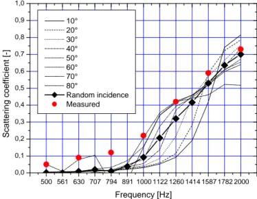
3.3.2. Scattering Coefficients

From the far field scattered pressure diagrams directional scattering coefficients are calculated using a discretisation of equation (21). If these are averaged for each source elevation over all

source azimuth angles, a scattering coefficient only depending on source elevation is obtained (Figure 6). Paris’ formula finally gives us the random incidence scattering coefficient (eq. (22)).

500 561 630 707 794 891 1000 1122 1260 1414 1587 1782 2000 0,0 0,1 0,2 0,3 0,4 0,5 0,6 0,7 0,8 0,9 1,0 S c a tt e ri n g c o e ff ic ie n t [-] Frequency [Hz] 10° 20° 30° 40° 50° 60° 70° 80° Random incidence Measured

Figure 6: 3D BEM calculated and measured scattering coefficients for the sine profile. (Measured values are

averaged values using the K.U.Leuven measurement technique12)

3.4. Comparison with Measured Scattering Coefficients

Real-scale measurements of the random incidence scattering coefficient of a sine shaped fibre cement circular plate have been performed12,13 according to the procedure described in ISO/DIS 17497-114. The measured sample is equally shaped compared to the 3D BEM model. Obtained random incidence scattering coefficients are compared to the calculated values in Figure 6. If the test sample were infinite then, according to equation (20), no propagating scattered waves can occur (except for the specular reflection) for frequencies below 960 Hz. Consequently, in this region the scattering coefficient should be zero. In the case of the finite BEM model, this holds for frequencies up to about 840 Hz, as long as the incidence angle is not too grazing. The overall higher values measured (compared to the calculated values) may be attributed to small variations in the reverberation room condition (temperature, humidity) and the parasitic scattering effect of the supporting base plate.

4

CONCLUSION

In order to compare scattering properties from different finite diffusers, the far field polar reflected pressure diagram needs to be known. The minimal distance away from the diffuser to reach this far field depends strongly on the geometry and the frequency of the incident wave. In this paper, guidelines to find this minimal far field distance in the case of a rigid flat infinite strip have been developed using an approach originally adopted by Kinsler. Respecting these guidelines, the far field reflected pressure field from a rigid circular surface with a sinusoidal height profile has been studied using a 3D BEM model. Comparisons are made to the case of an infinite sinusoidal surface and an equally sized rigid plane reflector. Finally, random incidence scattering coefficients are calculated and compared to real scale measurements. A good agreement has been found.

5

REFERENCES

1. E. Mommertz, Determination of scattering coefficients from the reflection directivity of architectural surfaces, Appl.Acoustics 60(2) (2000), p.201-203.

2. AES, Characterization and measurement of surface scattering uniformity, AES-4id-2001 in J.Audio Eng.Soc.49(3) (2001), p.148-165 / http://www.aes.org.

3. L. E. Kinsler, A. R. Frey, A. B. Coppens, and J. V. Sanders, Fundamentals of acoustics, 4th edition, John Wiley & Sons, Inc.(2000).

4. D. L. Smith, Discrete-element line arrays - Their modeling and optimization, J.Audio Eng.Soc.45(11) (1997), p.949-964.

5. M. S. Ureda, Line arrays: Theory and applications, AES 110th convention (2001), preprint #5304.

6. M. S. Ureda, Pressure response of line sources, AES 113th convention (2002), paper #5649. 7. L. Cremer and H. Müller, Principles and applications of room acoustics, Volume 1, Applied

Science Publishers, Essex, England (1982).Originally published in German (1978) by Hirzel Verlag, Stuttgart.

8. M. C. Junger and D. Feit, Sound, structures and their interaction, 2nd edition (1986), MIT press Cambridge (Mass).

9. F. M. Wiener, On the relation between the sound fields radiated and diffracted by plane obstacles, JASA 23(6) (1951), p.697-700.

10. H. Kuttruff, Room acoustics, 4th edition, Spon Press, London (2000).

11. R. L. Holford, Scattering of sound waves at a periodic, pressure-release surface: an exact solution, JASA 70(4) (1981), p.1116-1128.

12. L. De Geetere and G. Vermeir, Investigations on real-scale experiments for the measurement of the ISO scattering coefficient in the reverberation room, Proc.Forum Acusticum (2002), paper RBA-06-004-IP.

13. J. J. Embrechts, Practical aspects of the ISO procedure for measuring the scattering coefficient in a real-scale experiment, Proc.Forum Acusticum (2002), paper RBA-06-001-IP. 14. ISO, Acoustics - Measurement of the random-incidence scattering coefficient of surfaces,