Automatic Landmark Detection in 2D images: A tree-based approach with multiresolution pixel features

Automatic Landmark Detection in 2D images :

A tree-based approach with multiresolution

pixel features

R´emy Vandaele1,2_{, Rapha¨el Mar´ee}1_{, S´ebastien Jodogne}2_{, and Pierre Geurts}1

1

Systems and Modeling, Department of EE and CS & GIGA-R,

2 _{Department of Medical Physics, C.H.U.,}

University of Li`ege, Sart-Tilman, B34 4000 Li`ege, Belgium remy.vandaele@ulg.ac.be

Abstract. In this paper, we propose a new generic landmark detec-tion method for 2D images. Our soludetec-tion is based on the use of ensem-bles of Extremely Randomized Trees combined with simple pixel-based multi-resolution features. We apply our method on a novel dataset of mi-croscopic zebrafish images. This method was also tested on datasets of cephalometric images during the Automatic Cephalometric X-Ray Land-mark Detection Challenge 2014, where we were ranked first during the first phase, and second during the second phase.

1

Introduction

Landmark detection on 2D image consists in finding particular points in an image. These points are typically defined by specialists of a specific research area. Most of the time, this detection is the first step of a larger process. For example:

– In orthodontics, cephalometry is a particular process to analyze the human cranium. It consists in detecting landmarks and measuring the distances (or distance ratios) between these landmarks in order to detect possible problems or to plan intervention treatments [4].

– In toxicology and pharmacology, landmark detection is used to perform mor-phometric measurements of the skeleton of zebrafish embryos and describe the effects of chemical treatments or gene knock-downs [8]. Scientists are especially interested by the length of the cartilage and the angles formed by the landmarks.

– Landmark detection can also be used to perform image registration [9]. By keeping specific landmarks registered, specialists are sure of the soundness of their final registration.

– Landmark detection is also used in face recognition algorithms in order to ease the recognition procedure [6].

II

Typically, the detection of the landmarks is done manually, which makes it a very complicated and time-consuming task given the number of landmarks to annotate and the number of images involved in daily research of diagnostic rou-tine. There is therefore a strong interest to develop automated or semi-automated landmark detection methods.

The problem of landmark localization in cephalometric X-Rays has been extensively studied in the literature. Existing methods are typically based on the combination of template matching algorithms and prior knowledge information and differ mainly in the feature extraction methods (see [5] for a brief review). In contrast, our solution is based on the application of generic machine learning methods, in particular tree-based ensemble methods (e.g., Random Forests [1] or Extremely Randomized Trees [3]). Randomized decision forests have found many applications in computer vision, mainly because of their flexibility, robustness to irrevelant features, low computational complexity and high expressive power [2].

In this paper, we propose a novel method and try to detect landmarks on a novel dataset of microscopic zebrafish images. We first describe our algorith-mic solution and then evaluate its performances on our dataset through cross-validation.

2

Method

Following the work of [8] that performed detection of a small number of land-marks on small zebrafish microscopy datasets, we adopted a supervised learning approach that exploits the manually annotated images to train models able to predict landmark positions in new, unseen, images. In particular, a separate pixel classification model is trained for each landmark to predict whether a given im-age pixel corresponds to the position of this landmark or not. This model is trained from a learning sample composed of pixels extracted either in the close neighboorhood of the landmark or at other randomly chosen positions within the training images. Each pixel in the training sample is described by a vector of visual features at different resolutions.

The different steps of the algorithm for a single landmark are explained in the following subsections. This procedure is repeated for every landmark separately.

2.1 Extraction and description of pixels

Each observation in the training sample corresponds to a pixel at position (x, y) in one of the training images and is labeled into one class among {0, 1} and described by several input features. We described below successively the output class associated to each pixel, the input features used to describe them, and the pixel sampling mechanism.

Output classes. In principle, only one position in each image corresponds to the landmark, which means that if N training images are available, only N positive

III

examples will be available to train our pixel classification model. To extend the set of positive examples, we consider as positive examples all pixels that are at a distance at most R from the landmark, where R is a method parameter. More precisely, if the landmark is at position (xl, yl) in an image, then the output class

of a pixel at position (x, y) in the same image will be: – 1 if (x − xl)2+ (y − yl)2≤ R2,

– 0 otherwise.

Multi-resolution input features. A pixel at location (x, y) will be described by raw pixel values in a square subwindow of height and width 2W + 1 centered at the shifted position (x + tx, y + ty), where W , tx, and ty are method

parame-ters. Because of the introduction of the shift parameters tx and ty (that will be

tuned by cross-validation), the model is potentially able to detect the landmark based on a structure not necessarily centered at the pixel. The interest of these parameters will be illustrated in section 3.3.

In contrast to [8] where single-resolution features were extracted, in this work, we capture the context of the landmark at different scales and distances, training images are downsized to 6 different resolutions prior to the subwindows extraction and the 6 resulting feature vectors are concatenated. For our images of size m × n pixels, these resolutions will be:

m 2i ×

n

2i∀i ∈ [0, 5].

Pixels of a subwindow extending beyond the image limit will be set to zero. In total, each pixel will be described by an input feature vector of size 6×(2W +1)2_.

Fig. 1. On the left, the training subsampling scheme. On the right, a demonstration of the translation.

Pixel sampling scheme. Naively sampling pixels uniformly from the training images will give a very unbalanced classification problem. For example, for a

IV

radius R = 20 pixels, only 1256 observations correspond to positive examples, which is very small compared to the whole size of the images (2576 × 1932 pixels for our zebrafish images). To generate a more balanced training sample, we randomly select N pixels in each training image, where P % of these N pixels are selected among positive pixels and 100 − P % are selected among negative pixels.

In addition, we constrained the image area in which the negative pixels are selected by taking into account the fact that a landmark is located in close positions from one image to another. To confirm that, our experiments reported that each landmark is located in a specific region of the image of radius with size between 50 − 150pixels. At the prediction stage (see below), we will use this information to constrain the search for a landmark to a given subregion of the image around the average landmark position in the training images. Therefore, it is enough to put in the training sample only pixels that belongs to this region. Negative examples in each image will be selected uniformly at random at a distance of at most 400pixels around the landmark. This subsampling contrasts with [8] where pixels were sampled in the whole image during the training and the prediction phase.

2.2 Classification model training

To train the pixel classifier, we will use the Extremely randomized tree algorithm [3]. This method builds an ensemble of T fully developed decision trees grown each from the original training sample (i.e., without bootstrapping). At each node, the best split is selected among k features chosen at random, where k can take its value between 1 and m, with m the total number of features. For each of the k (continuous) features, a discretization threshold is selected at random within the range of variation of that feature in the subset of observations in the current tree node. The score of each pair of feature and threshold is computed and the best pair among the k is chosen to split the node. As a score measure, we use the Gini index reduction.

2.3 Landmark prediction

Let us denote by µl ∈ R2 and Σl ∈ R2×2 respectively the average and the

covariance matrix of the landmark positions across the training images and let us denote by σxland σylthe standard deviation of its x and y positions respectively

(i.e., the diagonal elements of Σl), also estimated from the training data. To

make prediction of the landmark position with our tree-based pixel classifier, we proceed as follows:

– We randomly draw 16σxlσyl pixel positions from the following multivariate

normal distribution:

V

– Each of the resulting pixels is classified by the tree ensemble and the final predicted landmark position is taken as the median position among the pixels that are predicted as being the landmark with the highest confidence by the tree-based model (i.e, which receives the highest number of votes for the positive class from the T trees in the ensemble).

This subsampling scheme allows to improve predictive performance by reducing the probability of generating spurious landmark predictions at irrelevant posi-tions in the images. It also considerably speedups the algorithm with respect to a full scan of all image pixels.

2.4 Method parameters and protocol The main method parameters are as follows:

– W , the size of the windows

– R, the distance to the interest point to decide on the training pixel output class.

– txand ty, the translation of the subwindows to define input features

– N , the number of pixels randomly sampled to train each landmark classifi-cation model.

– The percentage P of positive examples among the N pixels

– k the number of features selected at each node in the Extremely Randomized Trees algorithm

– T , the number of trees

During the validation, T was fixed to a default value of 500 and we used the suggested default value of k, which is the square root of the number of input features [3]. N was fixed to 500 and W to 8 in all our experiments. All other parameters were tuned by cross-validation. During this cross-validation, we separately optimized the different error criteria.

The parameter tuning was done in several stages as follows (for each land-mark of each dataset separately):

– The optimal values of txand ty were jointly tested in {8, 16, 32, 64, 128, 256}

(pix) for positive and negative translations using R = 10 and P = 33%. – R was then optimized in {2, 5, 7, 10, 12, 15, 17, 20, 25, 30} (pix) using P =

33% and the optimal values of tx and ty determined at the previous stage.

– Finally, P was optimized in {10, 20, 30, 33.33, 40, 50, 60, 70, 80,90} (%) with all other parameters set at their optimal values.

In total, this represents about 2000 cross-validation jobs for each criterion. We use the implementation of the Extremely Randomized Trees in scikit-learn [7] and our own python code for pixel and feature computation. Visual interpre-tation of the results was done using a web-based software for the visualization and analysis of large bioimages.

VI

3

Results

In this section, we carry out various experiments with our method on our ze-brafish dataset. After a description of this datasets and the evalution criteria, we first report in Section 3.2 the best results obtained on both problems when parameters are optimized by cross-validation. Then, we analyze in Section 3.3 the influence of the different steps of our method, in particular with respect to our previous work in [8].

Fig. 2. Typical landmark detection results. In green, ground truth data. In red, de-tected landmarks

3.1 Datasets

Our dataset (see Figure 2 for one example image for each dataset) has been collected by local experts and ground-truth (landmark positions) was created using a web-based annotation software. It is composed of 593 zebrafish images. All images are of size 1932 × 2576 pixels in 8 bits RGB values that we converted to grey value for our landmark detection method. There are 31 landmarks to detect on these images. Overall, it is a significantly larger dataset than the one used in [8] where authors detected only 4 landmarks in smaller datasets (±20 images)

As performance criteria, we considered 5 different criteria that seemed to be visually relevant to our image dataset: the number of landmarks detected with an error ≤ 20, 25, 30, 40 pixels and the euclidean distance from the predicted landmark to its true position.

3.2 Best results

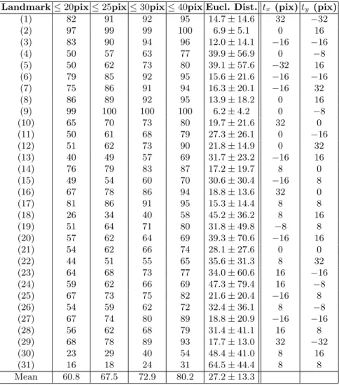
Table 1 report our best performances for all landmarks and criteria respectively on our zebrafish dataset. We used the first 493 images for training our model

VII

and the remaining 100 images for testing. Parameters were tuned on the training data by 10-fold cross-validation as explained in Section 2.4.

Table 1. Results on all landmarks for the zebrafish dataset. Note: tx and ty are the

best translation parameters obtained for the 25pix criterion

Landmark ≤ 20pix ≤ 25pix ≤ 30pix ≤ 40pix Eucl. Dist. tx (pix) ty (pix)

(1) 82 91 92 95 14.7 ± 14.6 32 −32 (2) 97 99 99 100 6.9 ± 5.1 0 16 (3) 83 90 94 96 12.0 ± 14.1 −16 −16 (4) 50 57 63 77 39.9 ± 56.9 0 −8 (5) 50 62 73 80 39.1 ± 57.6 −32 16 (6) 79 85 92 95 15.6 ± 21.6 −16 −16 (7) 75 86 91 94 16.3 ± 20.1 −16 32 (8) 86 89 92 95 13.9 ± 18.2 0 16 (9) 99 100 100 100 6.2 ± 4.2 0 −8 (10) 65 70 73 80 19.7 ± 21.6 32 0 (11) 50 61 68 79 27.3 ± 26.1 0 −16 (12) 51 62 73 90 21.8 ± 14.9 0 32 (13) 40 49 57 69 31.7 ± 23.2 −16 16 (14) 76 79 83 87 17.2 ± 19.7 8 0 (15) 49 54 60 70 30.6 ± 30.4 −16 8 (16) 67 78 86 94 18.8 ± 13.6 32 0 (17) 81 86 91 95 15.3 ± 14.4 8 8 (18) 26 34 40 58 45.2 ± 36.2 8 16 (19) 51 64 71 80 31.8 ± 49.8 −8 8 (20) 57 62 64 69 39.3 ± 70.6 −16 16 (21) 54 62 66 74 28.1 ± 27.6 0 0 (22) 44 51 55 65 35.6 ± 31.3 8 32 (23) 64 68 73 77 34.0 ± 60.6 16 −16 (24) 59 62 66 69 47.3 ± 79.4 16 −8 (25) 67 73 75 82 21.6 ± 20.4 −16 8 (26) 54 59 62 72 32.4 ± 36.1 8 −8 (27) 67 74 80 89 18.8 ± 20.9 −16 −16 (28) 56 62 68 79 31.4 ± 41.1 16 8 (29) 68 78 89 93 17.7 ± 13.0 32 −32 (30) 23 29 40 54 48.4 ± 41.0 8 16 (31) 16 18 24 31 64.5 ± 44.4 8 8 Mean 60.8 67.5 72.9 80.2 27.2 ± 13.3

Results on both datasets differ from one landmark to another but they are rather good from a visual perpective, as we show in 2.

3.3 Experiments

In this section, we carry out several experiments to show the influence of the different steps of our method and hereby motivate our design choices. More

VIII

precisely, we compare four different methods, obtained by disabling one or several steps of our full proposal. The compared methods are as follows (see Table 3 for a summary):

– METH: our complete method as described in Section 2.

– NOTR: The method METH with translations disabled (tx= ty = 0)

– 1RES: The method NOTR with features extracted at a single resolution instead of 6. The keep the number of features approximately fixed, we in-creased the size of the single resolution window to W = 20 and used the raw pixel values in this window as input features.

– GRID: The method NOTR but with the sampling of the observations inde-pendent of the distribution of the landmark positions in the training images. During training, negative observations are unformily drawn from the whole image. During prediction, 10,000 observations are extracted on a regular grid covering the whole image. This sampling scheme is similar to the one used in [8]1_.

Average results over all landmarks2 _{are reported for these four methods in}

Table2. They were obtained by 10-fold cross-validation over 100 randomly se-lected images. For each of these experiments, all parameters are set to a default value, namely 50 trees, 300 observations per images, R = 10, and P = 33%. To obtain a fair comparison, the number of predicted observations was fixed to 10.000 for all methods. For METH, the translation parameters were determined by internal 10-fold cross-validation.

The comparison between NOTR and GRID shows that our adaptive sampling scheme is much better that uniform sampling, according to all criteria and on both datasets. There is also a clear performance gain when going from 1RES to NOTR on both datasets and all criteria. For a fixed number of features, it is thus more important to capture information at multiple resolutions than to extend the window size. The performance further increases when going from NOTR to METH, highlighting the interest of the translation. Overall, the best results are obtained on both datasets when using multi-resolution features, adaptive subsampling, and translation.

Table 2. Evolution of the performances with the sampling scheme for the zebrafish dataset

Experiment ≤ 20pix ≤ 25pix ≤ 30pix ≤ 40pix Eucl. Dist.

GRID 48.8 56.3 62.2 71.2 48.7

NOTR 54.1 61.0 66.1 73.9 35.0

1RES 38.7 42.9 46.9 53.3 71.2

METH 60.2 67.4 71.9 79.7 29.3

1

In [8], we did a full scan of the image at the prediction stage but the computation cost of a full scan would be too high on our two datasets here, given the higher resolution of the images.

2

IX Table 3. Summary of the experiments

Experiment Subsampling Multi-Resolution Translation

GRID No Yes No

NOTR Yes Yes No

1RES Yes No No

METH Yes Yes Yes

4

Conclusion

We showed that it was possible to accurately detect some of the landmarks using a combination of Extremely Randomized Forests and simple features. In particular, we have shown the advantadge of using our multi-resolution approach and our subsampling scheme. High level features such as Zernike moments can accurately describe an image or a window, but they are slow to compute, which could be detrimental in some applications. The main advantage of our approach with respect to existing works is its simplicity and efficiency. We also want to point out the versatility of our approach, able to suit very various kinds of landmark detection problems: the exact same method allowed us to reach a first and second place during the Automatic Cephalometric X-Ray Landmark Detection Challenge 2014.

In future work, we believe that further improvement could probably be ob-tained by taking into account the relative positions of the landmarks either directly during the training or during the prediction stage. We have made some experiments in this direction but we were not able to improve with respect to the results reported here. Further improvement could also be brought by considering different values of W at each of the different resolutions or different feature sets. For the zebrafish dataset, additional information could also be brought by using the RGB pixel values instead of just considering luminance.

We are also interested in using a similar methodology to detect landmarks on 3D volumes. Cephalometric landmark detection on 3D volumes could be one of the interesting topics.

Acknowledgment

Double blind

References

1. Leo Breiman. Random forests. Machine learning, 45(1):5–32, 2001.

2. A. Criminisi and J. Shotton. Decision Forests for Computer Vision and Medical Image Analysis. Springer, 2013.

3. Pierre Geurts, Damien Ernst, and Louis Wehenkel. Extremely randomized trees. Machine learning, 63(1):3–42, 2006.

X

4. Vicente Grau, M Alcaniz, MC Juan, Carlos Monserrat, and Christian Knoll. Auto-matic localization of cephalometric landmarks. Journal of Biomedical InforAuto-matics, 34(3):146–156, 2001.

5. Amandeep Kaur and Chandan Singh. Automatic cephalometric landmark detection using zernike moments and template matching. Signal, Image and Video Processing, pages 1–16, 2013.

6. M Pamplona Segundo, Luciano Silva, Olga Regina Pereira Bellon, and Chau˜a C Queirolo. Automatic face segmentation and facial landmark detection in range images. Systems, Man, and Cybernetics, Part B: Cybernetics, IEEE Transactions on, 40(5):1319–1330, 2010.

7. F. Pedregosa, G. Varoquaux, A. Gramfort, V. Michel, B. Thirion, O. Grisel, M. Blon-del, P. Prettenhofer, R. Weiss, V. Dubourg, J. Vanderplas, A. Passos, D. Courna-peau, M. Brucher, M. Perrot, and E. Duchesnay. Scikit-learn: Machine learning in Python. Journal of Machine Learning Research, 12:2825–2830, 2011.

8. Olivier Stern, Rapha¨el Mar´ee, Jessica Aceto, Nathalie Jeanray, Marc Muller, Louis Wehenkel, and Pierre Geurts. Automatic localization of interest points in zebrafish images with tree-based methods. In Pattern Recognition in Bioinformatics, pages 179–190. Springer, 2011.

9. Barbara Zitova and Jan Flusser. Image registration methods: a survey. Image and vision computing, 21(11):977–1000, 2003.