DEVELOPMENT OF A NEW DESIGN METHOD
FOR THE CROSS-SECTION CAPACITY OF
STEEL HOLLOW SECTIONS
A thesis
Submitted in fulfillment of the requirements for the degree
Of
Doctor in Applied Sciences
By
JOANNA NSEIR
MEMBERS OF THE JURY
M. Philippe Rigo (President of the jury) University of Liège, Department Argenco Chemin des Chevreuils, 1 B52
B – 4000 LIEGE – Belgium M. Jean-Pierre Jaspart (Supervisor) University of Liège, Department Argenco Chemin des Chevreuils, 1 B52
B – 4000 LIEGE – Belgium M. Fadi Geara (Supervisor)
Saint-Joseph University USJ, Engineering Faculty ESIB Technologies and Sciences Campus, Mar Roukoz, Mkalles Riad El Solh, Beyrouth, 11 07 2050 – Lebanon
M. Nicolas Boissonnade (Supervisor)
University of Applied Sciences of Western Switzerland – Fribourg Bd de Perolles 80 – CP 32
CH-1705 Fribourg – Switzerland M. Leroy Gardner
Imperial College London
Department of Civil and Environmental Engineering South Kensington Campus, London, SW7 AZ, UK M. Alfred Seyr
Voestalpine Krems GmbH
Schmidhüttenstrasse 5, Krems Austria M. Jean-Francois Demonceau
University of Liège, Department Argenco Chemin des Chevreuils, 1 B52
‘Il faut avoir beaucoup étudié pour savoir peu’
ACKNOWLEDGEMENTS
I would like to thank all the people who contributed in some way to the work described in this thesis. First and foremost, I would like to express my special appreciation and thanks to my supervisor M. Nicolas Boissonnade, who has been a tremendous mentor for me. I would like to thank you for encouraging my research and for allowing me to grow as a research scientist. Your advice on both research as well as on my career have been priceless. I would also like to express my sincere gratitude to my directors, M. Jean-Pierre Jaspart and M. Fadi Geara who have both become role models for me. Thank you for your encouragements, constructive moments and advices necessary for my progress through my doctoral program.
I also want to thank the jury, M. Philippe Rigo, M. Leroy Gardner, M. Alfred Seyer and M. Jean-francois Demonceau, for dedicating their time and lending me their expertise in order to accomplish this work, for that i am very honored.
I would like to thank the universities who accompanied and supported me during my thesis. I owe my gratitudes to the University of Applied Sciences of Western Switzerland, Fribourg (HEIA-FR), Liege University, Belgium (Ulg) and Saint-Joseph University, Lebanon (USJ). This project was financed by CIDECT and AUF. I could not have completed my work without their financial support. I owe also gratitude to Voestalpine Krems for supplying the necessary specimens for my experiments.
A big thank you to all my colleagues and friends Raja, Laurent, Julien, Vincent, Yongzhen, Raphael, Delphine, Ana, Jonathan and the Lab technicians Jean-Paul and Dominique. I had an enormous pleasure to work and interact with all of you in a very good atmosphere.
Many thanks for Yanis Schaller. Thank you for helping me and bearing with me during my experimental tests. Although I was always leaving a huge mess behind me in the lab, you supported me and helped me through my campaign.
Many Thanks to Elsy and Marielle, my two steel PhD colleagues for the lovely moments we spent together and the long working days we had in our messy office. We shared lot of great funny moments during our stay in Switzerland and in many congresses.
Thanks to Lionel Moreillon who helped me in the test set-up drawings of my thesis and who gave me and taught me a great experience in research during my masters, which was an encouragement for me to start my PhD.
I would particularly like to thank Joao Tomas Silva for his continuous support during my thesis. Thank you Joao for being my little brother (sorry big) and thank you for helping me during my hardest moments of my PhD. I would never forget you standing by my side and helping me in the Lab until 4am in the morning.
I am most grateful for all the support I received from my family. Special thanks to mom and dad, for being always beside me and supporting me in every task i was involved in. Thanks mom for your continuous prayers for me and sorry for making you worry about me during my hardest times in my PhD. Dad, thank you for always making me feel that you are proud of me no matter what, and always supporting me.
Finally, and last but certainly not least in any way, my deep gratitudes to my dear fiancé Simon Yared for his massive support and infinite patience all along my PhD period. I am lucky to have met Simon and i thank him for his love, friendship and unyielding support.
Joanna Nseir, June 2015 .
ABSTRACT
The cross-sectional behaviour of steel sections can be shown to be influenced by two extreme behaviors: the resistance and the instability. These boundaries are accounted for in current standards through a classification system consisting on rules depending on the cross-section dimensions. For example, in EN 1993-1-1, classes are defined spanning from stocky sections (class 1) able to develop their full plastic capacity, to slender sections (class 4) for which the effective properties are used with the use of the effective width method (EWM). However, for cold-formed steel sections, characterized by a non-linear material law, the cross-section resistance can go beyond its plastic capacity due to strain hardening effects. Moreover, with the emergence of high strength steel (i.e. cross-sections falling into class 4) and more complex cross-section shapes, the effective width method is becoming too complicated. Many other reasons and discrepancies are making the cross-section classification too complex and inconsistent.
The Overall Interaction Concept (OIC) stands as a new design approach that aims at a straightforward design check of the stability and resistance of steel cross-sections. Based on the use of a generalized relative slenderness and so-called interaction curves, it can be applied to any type of cross-section, further includes potential non-linear material behaviour and covers combined loading cases. The main aim of this thesis is to develop and propose OIC interaction curves dedicated to steel hollow sections subjected to various load cases.
A test program was carried out as a part of a European project named ‘HOLLOPOC’ to investigate the cross-sectional behavior of cold-formed hot-finished and hot-rolled square, rectangular and circular sections. 57 cross-sections tests including simple and combined load cases were performed. Besides, a finite element model was developed and calibrated on the basis of the tests, and its accuracy was seen to be sufficient to subsequently undergo an extensive numerical parametric study for hot-rolled and cold-formed cross-sections, leading to over than 40 000 numerical results. Based on these computations, design proposals were made within the context of the Overall Interaction Concept, using an extension of the Ayrton-Perry approach. Finally, a validation of the proposed formulae was made through a comparison with existing approach and worked examples were presented, in order to illustrate (i) the application of the method and (ii) its benefits in comparison to application of current EC3 rules.
TABLE OF CONTENTS
ACKNOWLEDGEMENTS ...III ABSTRACT ... V NOTATIONS ... XIV 1. INTRODUCTION ... 22 1.1. Context ... 221.2. Scope and objectives of the thesis ... 25
1.3. Outline of the thesis ... 28
2. STATE OF THE ART ... 30
2.1. Literature review on local buckling ... 30
2.1.1. Brief historical review ... 30
2.1.2. Elastic behavior of plates under edge compression ... 31
2.1.2.1. Elastic buckling stress of plates ... 33
2.1.2.2. Elastic local buckling coefficient of plates and sections ... 38
2.1.2.2.1. Plate buckling coefficient ... 38
2.1.2.2.2. Cross-sectional buckling ... 42
2.1.3. Post-buckling behavior and effective width methods ... 47
2.1.4. Influence of residual stresses and initial imperfections on plate buckling ... 54
2.2. Brief review of plastic theory ... 56
2.3. Available methods for the determination of buckling loads ... 58
2.3.1. Finite element method ... 58
2.3.2. Plastic mechanisms ... 59
2.3.3. Ultimate buckling curves ... 61
2.4.1. Cross-section classification concept ... 62
2.4.2. Shortcomings of the classification system ... 75
2.4.2.1. Classification system background and emergence of non-linear materials ... 75
2.4.2.2. Emergence of high strength steel ... 75
2.4.2.3. Boundary conditions and post-buckling reserves ... 76
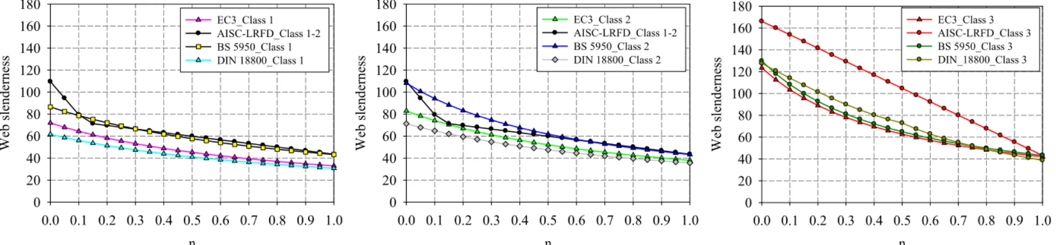
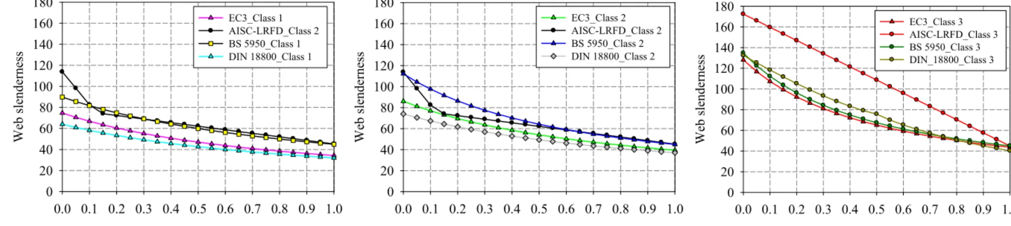
2.4.2.4. Slenderness definition ... 77
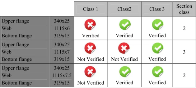
2.4.2.5. Gap of resistance between class 2 and class 3 ... 81
2.4.2.6. Errors and contradictions in table 5.2 of EN 1993-1-1 ... 83
2.4.2.7. Unconformity in the determination of the class 4 plate slenderness limit ... 89
2.4.2.8. Other inconsistencies ... 91
2.5. Design alternatives in development – Use of modern tools ... 92
2.5.1. Direct strength method – DSM ... 93
2.5.1.1. Introduction ... 93
2.5.1.2. Cross-section slenderness definition ... 93
2.5.1.3. Base curves ... 94
2.5.1.3.1. Sections in compression ... 94
2.5.1.3.2. Beams ... 96
2.5.1.3.3. Beam-columns ... 97
2.5.1.4. Practical and theoretical advantages and limitations of DSM ... 99
2.5.2. The continuous strength method – CSM ... 101
2.5.2.1. Introduction ... 101
2.5.2.2. Cross-section slenderness definition ... 102
2.5.2.3. Strain ratio and material model ... 102
2.5.2.4. Base curve ... 105
2.5.2.5. Cross-section bending and compression resistance ... 107
2.5.2.6. Cross-section beam-column resistance ... 108
2.5.2.7. Simplified CSM for beam-column ... 109
2.5.2.8. Practical and theoretical advantages and limitations ... 109
2.6. Summary ... 110
3. EXPERIMENTAL INVESTIGATIONS ... 112
3.2. Test program ... 112
3.3. Preliminary measurements ... 116
3.3.1. Cross-sectional dimensions ... 116
3.3.2. Geometrical imperfections ... 118
3.3.3. Residual stresses ... 120
3.3.3.1. Fabrication process and type of residual stresses ... 120
3.3.3.2. Experimental techniques ... 125
3.3.3.3. Residual stresses measurements ... 126
3.3.4. Material properties ... 143
3.3.4.1. Tensile tests ... 143
3.3.4.2. Stub column tests ... 146
3.4. Cross-section tests ... 152
3.4.1. Testing procedure and results ... 152
3.4.2. Comparison with EC3 predictions and discussion ... 161
3.5. Collection of existing results ... 167
3.6. Summary ... 171
4. NUMERICAL INVESTIGATIONS ... 172
4.1. General ... 172
4.2. Validation against test results ... 172
4.2.1. UAS Western Switzerland Fribourg campaign ... 172
4.2.1.1. Numerical model – Features and characteristics ... 172
4.2.1.1.1. Elements and meshing ... 172
4.2.1.1.2. Loading and support conditions ... 176
4.2.1.1.3. Material modeling and residual stresses ... 178
4.2.1.2. Validation: FE results vs. test results ... 180
4.2.2. TU Graz campaign ... 186
4.2.2.1. General scope of the study ... 186
4.2.2.2. Numerical model – Features and characteristics ... 187
4.2.2.2.2. Loading and support conditions ... 188
4.2.2.2.3. Material modelling and residual stresses ... 188
4.2.2.3. Validation: FE results vs. test results ... 190
4.3. Numerical parametric study ... 192
4.3.1. Meshing, loading and support conditions ... 192
4.3.2. Initial geometrical imperfections ... 193
4.3.2.1. Introduction ... 193
4.3.2.2. Initial imperfection sensitivity study ... 196
4.3.2.2.1. Local imperfect shape for tested cross-sections ... 196
4.3.2.2.2. Local imperfect shape study on other cross-sections ... 205
4.3.2.2.3. Imperfection amplitude study ... 209
4.3.2.2.4. Final selection of geometrical imperfections and recommendations for FE modelling ... 211
4.3.3. Load-path sensitivity ... 213
4.3.4. Numerical study of hot-rolled sections ... 222
4.3.4.1. Material law and residual stresses ... 222
4.3.4.2. Parameters considered ... 224
4.3.5. Numerical study of cold-formed sections ... 227
4.3.5.1. Material law and residual stresses ... 227
4.3.5.2. Cross-sections and parameters considered ... 229
4.4. Determination of R-factors involved in the OIC approach ... 230
4.4.1. Determination of RRESIST ... 230
4.4.2. Determination of RSTAB ... 240
4.5. Gathered experimental data vs. FE results ... 243
4.6. Summary ... 245
5. DESIGN PROPOSAL – OVERALL CROSS-SECTION DESIGN ... 246
5.1. Identification of key parameters ... 246
5.1.1. Influence of yield stress, geometrical imperfections and residual stresses ... 246
5.1.2. Influence of material law ... 247
1.1.1. Influence of warping and second-order effects ... 252
5.2. Towards a design proposal: Mechanical background ... 253
5.2.1. Empirical formulations ... 254
5.2.2. Merchant-Rankine formulation ... 255
5.2.3. Ayrton-Perry format ... 257
5.2.4. Adopted formulation ... 259
5.3. Determination of interaction curves ... 261
5.3.1. Simple load cases ... 262
5.3.1.1. Axial compression ... 262 5.3.1.1.1. Hot-rolled sections ... 262 5.3.1.1.2. Cold-formed sections ... 268 5.3.1.2. Major-axis bending ... 277 5.3.1.2.1. Hot-rolled sections ... 277 5.3.1.2.2. Cold-formed sections ... 281 5.3.1.3. Minor-axis bending ... 287 5.3.1.3.1. Hot-rolled sections ... 287 5.3.1.3.2. Cold-formed sections ... 290
5.3.2. Combined load cases ... 292
5.3.2.1.1. Hot-rolled sections ... 292
5.3.2.1.2. Cold-formed sections ... 306
6. ACCURACY OF PROPOSED MODELS – COMPARISON WITH ACTUAL RULES ... 324
7. SUMMARY AND RECOMMENDATIONS ... 344
8. WORKED EXAMPLES ... 349
8.1. Introduction ... 349
8.2. Square hollow section: SHS 250x5 ... 349
8.2.1. Cross-section and member properties ... 349
8.2.2.1. Eurocode 3 approach ... 350
8.2.2.2. OIC approach ... 355
8.3. Rectangular hollow section: RHS 200x100x5 ... 356
8.3.1. Cross-section properties... 356
1.1.2. Cross-section resistance ... 357
1.1.2.1. Eurocode 3 approach ... 357
8.3.1.1. OIC approach ... 360
8.4. Summary of results and conclusions ... 361
9. CONCLUSIONS ... 362
9.1. General ... 362
9.2. Personal contributions ... 363
9.3. Suggestions for further studies ... 365
10. REFERENCES ... 368
11. ANNEXES ... 377
11.1. Annex 1 – Geometrical dimensions ... 377
11.2. Annex 2 – Detailed results of tensile tests ... 379
11.3. Annex 3 – Detailed results of residual stresses determination ... 384
11.4. Annex 4 – Detailed results of geometrical imperfection measurements ... 394
11.5. Annex 5 – Detailed results of stub column tests ... 396
11.6. Annex 6 – Detailed cross-section test results and comparison with FE results ... 433
LISTE OF FIGURES ... 608
NOTATIONS
Abbreviations:
AISC American Institue of Steel Construction CF Cold-Formed
CHS Circular Hollow Section CSM Continuous Strength Method DSM Direct Strength Method
EC3 Eurocode 3
EN European Standard
EWM Effective Width Method
FE Finite Element
GMNIA Geometrically, materially nonlinear analysis with imperfections HF Hot-Finished
HR Hot-Rolled LBA Linear buckling analysis
LC Load Case
LVDT Linear Variable Displacement Transducer MNA Materially nonlinear analysis
OIC Overall Interaction Concept PNA Plastic Neutral Axis
RHS Rectangular Hollow Section SHS Square Hollow Section 1S Upper LVDT at position 1
2S Upper LVDT at position 2 3S Upper LVDT at position 3 4S Upper LVDT at position 4 1B Bottom LVDT at position 1 2B Bottom LVDT at position 2 3B Bottom LVDT at position 3 4B Bottom LVDT at position 4 Latin letters:
a Length of local panel
a Measured deflection of the strip (only used in section 3.3.3)
a Initial imperfection amplitude (only in section 4.3.2)
B Section width
b Width of local panel
be Effective width
bf width of the flange
dz, dy Distance between LVDTs along z-axis and y-axis respectively
dy1, dy2 Distance between LVDTs and the centerpoint of the application load along y-axis
dz1, dz2 Distance between LVDTs and the centerpoint of the application load along z-axis
ey Excentricity in y-axis direction
ez Excentricity in z-axis direction
E Young’s modulus of elasticity
Em Young’s modulus of elasticity, mean
ESG Young’s modulus from strain gauges
f Stress
fu_flat Material ultimate stress of the flat region
fu_corner Material ultimate stress of the corner region
fu,m Ultimate stress, mean
fcsm Limiting CSM stress
fy Material yield stress
fym Materil yield stress, mean of yield plateau
fu Material ultimate stress
fmax Ultimate tensile stress
Fexp Applied force at ultimate load for experimental tests
FFE Applied force at ultimate load for Finite Element simulations
Fpl_actual Plastic load based on actual properties
Fpl_nom Plastic load based on nominal properties
hw Height of the web
H Section depth
Iy Moment of inertia about the strong axis
Iz Moment of inertia about the weak axis
k Correction factor (only used in section 3.3.4.2)
k, kσ Plate buckling coefficient
lfinal Final length measured by the extensometer
linitial Initial length measured by the extensometer
L Length Larc_i Arc length at the inner surface
Larc_f Arc length at the outer surface
Larc_m Arc length at the neutral axis
Larc_final final arc length
m Number of sine waves of a panel in the x direction
my Normalized major-axis bending moment
mz Normalized minor-axis bending moment
MEd Design value of the acting bending moment
Mel Elastic cross-section resistance for pure bending moment
Mpl Plastic cross-section resistance for pure bending moment
My Bending moment about the strong axis (y-y)
Mz Bending moment about the weak axis (z-z)
n Number of sine waves of a panel in the y direction (used only in section 2.1)
n Normalized axial force, equal to N N / pl
N Axial force
Npl Plastic cross-section resistance for pure axial force
NEd Design value of the acting axial force
Nu Ultimate compression load
Nx Compression load
P Compression force
Pcrl Elastic local buckling load
Pcrd Elastic distortional buckling load
Pcre Elastic global buckling load
Pnd Maximum distortional buckling strength
Pne Maximum global buckling strength
Ptest Test load
Py Squash load
r Corner radius
Re External curvature radius
Ri Interal curvature radius
Rm curvature radius at the neutral axis
Rm_final Final mid-thickness radius of curvature
RULT Ultimate load multiplier
RRESIST Resistance load multiplier
RSTAB Critical load multiplier
t Thickness
tf Thickness of the flange
tw Thickness of the web
w Deflection of local panel
Wpl Plastic section modulus
Wel Elastic section modulus
Greek letters:
Angle of curvature
Degree of bi-axiality
CS Cross-section imperfection factor
Factor relative to the instability limit
βcrl Critical elastic local buckling magnitude under combined P-M-M resultant;
Exponent factor to the level of axial forces n
, α Constants determined based on the manufacturing process (only in section 4.3.2)
b Bottom displacement
δc Corrected stub column end-shortening
δLVDT End-shortening recorded by LVDTs
TOT Total displacement
u Upper displacement Strain of 235 y f CSM CSM strain lb Failure strain lb Critical strain
u Material ultimate strain
x Strain at position x
y Material yield strain
η Generalized imperfection factor
yb Bottom rotation around y-axis
yu Upper rotation around y-axis
zb Bottom rotation around z-axis
zu Upper rotation around z-axis
Relative slenderness
End of plateau slenderness
λcs Cross-section slenderness
λCS,N Cross-section slenderness relative to a compression load case
λp plate slenderness
ξf Clamping coefficient for flange
ξw Clamping coefficient for web
σ Stress
σ0.2 0.2% proof stress
σcr Critical stress
σext External stress
σmax Maximum edge stress
σrc Stress due to residual stresses
σult Ultimate stress
σy Yield stress
Poisson’s ratio
ϕ Variable accounted for in the Ayrton-Perry formula
Buckling reduction factor
cs Cross-section reduction factor
N
Buckling reduction factor in case of compression
Fraction of yield stress in tension
1. Introduction
1.1. Context
The use of hollow structural steel has been increasing in the past few years. Although the price per ton of hollow sections is much higher than that of open profiles, their aesthetic appeal and their enhanced static values allow lighter construction and economic structures. Long-span roof structures and industrial buildings are increasingly designed with structural hollow sections. Modern architecture is dominated by tubular cold-formed structure, while industrial structures are dominated by hot-rolled tubular sections. Figure 1 shows some astonishing tubular structures made around the world.
Figure 1– Australia stadium (Australia), the kelpies (Scotland), Liege Guillemins railway station (Belgium), Madrid Barajas international airport (Spain), London eye (Britain).
The increase use of tubular sections is not only due to their excellent architectural aspect but also to their economic advantages in comparison with open sections. Square, rectangular or round cross-sections have outstanding static properties which can be presented as follows: (i) Their excellent behavior towards global buckling, lateral torsional buckling and torsion
is due to their closed shape and the favourable distribution of material around the longitudinal axis of the section;
(ii) The use of the internal volume to increase the load bearing capacity of the column by filling it with concrete;
(iii) The corrosion protection can be applied economically compared to open sections considering that hollow sections have smaller and smoother surfaces without any sharp edges.
However, the use of hollow sections present an inconvenient for the case of elements for which bending is the primary action since the uniform distribution of material around the longitudinal axis of the section would constitute a handicap compared to open sections ( H or I ). Indeed, for bending, hollow profiles have generally a high sufficient thickness ( due to both webs ) to absorb shear stresses, but the flange thicknesses are not economically sufficient to absorb the normal stresses due to bending. Therefore, the hollow profiles are undeniably the ideal profiles for columns while open profiles are more suitable for the beams. However, the occurrence of lateral torsional buckling in open sections may change this last conclusion and make the hollow profiles best suited to be used for both columns and beams. The buckling behavior of hollow profiles becomes even better when the material is distributed as far as possible from the longitudinal axis of the section. For an identical area, one comes to consider that economy will lead to hollow profiles of greater widths and smaller thicknesses. The resulting thinness of the plates may however lead to another phenomenon of instability named ‘local buckling’ which is the main issue studied in this thesis. Moreover, the increase in yield stress plays a similar role as the decrease in plates’ thicknesses and will also trigger local buckling.
The modern trend is to produce thin-walled hollow sections and high yield strength with significant interaction between local buckling and global buckling. This thesis is only concerned with the study of the behavior of hollow cross-section capacities which will endure either material yielding or local buckling.
For what concerns local buckling, most of the actual codes rely on the effective width concept, and the classification system which propose so-called /b t limit ratios that each of the section’s wall should fulfill to be considered as non-affected by early local buckling. Besides, recently developed alternatives based on the use of more sophisticated tools [1] or on a continuous relationship between strains and plate slenderness [2] have been suggested. From a practical point of view, these codes and methods however suffer from a series of issues and inadequacies. Amongst them, the handling of local buckling may appear as the one causing most problems; it is indeed usual to adopt a design resistance formula in accordance with the proneness of the cross-sections to suffer from early local buckling: the earlier the occurrence of local buckling is expected to occur, the more restricted the design rules. In Eurocode 3, this is accounted for through an additional step prior to the verification process that consists in the classification of the cross-section. According to the class of the section1, different sets of formulae are to be used for the design checks of both sections and members, i.e. plastic or elastic equations. it has been shown [3] that several values of the /b t limit
ratios of Eurocode 3 are often misleading, further to suffering from a lack of mechanical background. Moreover, the concept of classes, as it is defined – discrete and artificial – generates a gap of resistance at the class 2-3 border, which is mechanically meaningless and unacceptable.
Recently, improvements have been brought to the European standards, in terms of corrected /
b t tables and of additional rules allowing for a linear transition along the class 3 ranges. Although reflecting the actual best knowledge in this field, these design rules still deserve improvements for situations where instability effects are important [4]. Also, in the particular case of plastic and compact sections, several research works suggest that a rational exploitation of strain hardening results in a better prediction of observed behavior and potentially leads to material savings, especially for cold-formed or stainless steel profiles but also for hot-rolled members [5].
Therefore, the aim of the research works presented herein is to contribute in improving this situation and proposing a new design approach replacing the actual classification system, leading to a more mechanical and rigorous approach. This approach would treat accurately
1 The class of a section is governed and defined by the class of its worst (i.e. weakest) element: in Eurocode 3,
the occurrence of local buckling and material yielding in short hollow members - in which only local buckling instability might develop - and would allow for a proper interaction between stability (buckling) and resistance (material yielding). This approach is named the Overall Interaction Concept (OIC) and will be presented in the following section.
1.2. Scope and objectives of the thesis
The basis of the Overall Interaction Concept depicted herein lies in the well-known interaction between the two main phenomena influencing the carrying capacity of structural members: resistance and instability. The behavior of a real cross-section is therefore influenced by both aspects, acting as upper bounds of the real behavior, as well as by initial imperfections (e.g. out-of straightness, residual stresses, non-homogenous material…). In this context, the accurate treatment of the interaction is a key point for a realistic prediction of the section’s resistance. No recognized general theoretical background has been established to organize and unify the handling of this crucial interaction in a global way. However, recent developments ( [4] & [6] ) have offered a glimpse that such an ambitious general approach can fill this fundamental gap of knowledge: the “Overall Interaction Concept”. Despite its formal simplicity, the potential of the OIC is such that all structural sections and members, whatever the material, could be treated with an identical general, global, accurate yet simple and sound-based background.
The proposed approach relies on the generalization of the relative slenderness concept, and on establishing this parameter as the key to rule the interaction. This concept of relative slenderness is familiar to structural engineers, and is widely used nowadays to deal with flexural buckling behavior for example. It is suggested within the OIC to drastically enlarge the field of application of this slenderness-related approach through the generalization of the idea of relative slenderness as follows:
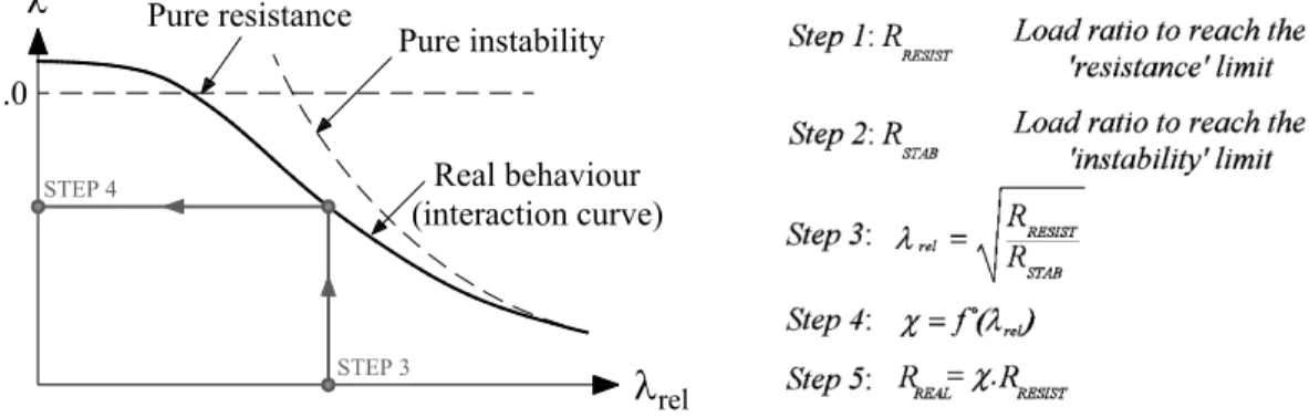
RESIST rel STAB R R l = (1)
where RRESIST represents the factor by which the initial loading has to be multiplied to reach the pure resistance limit, while RSTAB is the factor used to reach the buckling load of the ideal
rel STEP 3 STEP 4 1.0 Real behaviour (interaction curve) Pure resistance Pure instabilityFigure 2 – Principles and application steps of proposed “Overall Interaction Concept”. Doing so allows the generalized relative slenderness to take a non-dimensional balance between the relative influences of instability and resistance, and makes it capable of dealing with combined loading situations or cross-sectional ( local ) instability effects as well. Once determined, this rel value is further used in the design procedure to get into a so-called “interaction curve” ( also sometimes referred to as “buckling curve” ) and leads to the determination of a “” value ( see Figure 2 ). This value ( analogous to the one used in Eurocode 3 ), which may also be called “reduction factor”, represents the penalty due to instability effects on the pure resistant behavior, and can obviously only be lower than 1.0. Then, the final resistance is evaluated as .RRESIST; Figure 2 further illustrates the proposed approach and its application steps.
This rather simple procedure can be applied to many situations within structural engineering – e.g. member buckling, cross-sectional resistance… – regardless of the material behavior, and acts as a general approach to each design situation where instability affects the resistance. Therefore, the prime aim of this thesis is to investigate the behavior of steel hollow sections and propose a suitable new design curves for the prediction of their cross-section capacities, through a new concept termed the Overall Interaction Concept, OIC. The main goals can be subdivided into further sub-sections consisting in:
(i) A comprehensive literature survey on the local buckling, plastic design history, actual treatment of the cross-section resistance and existing alternatives;
(ii) An experimental study of the behavior of cold-formed, hot-rolled and hot-finished square, rectangular and circular sections under simple and combined loading. The
identification of a plastic collapse mechanism relative to short members with stocky sections, from a local buckling instability collapse relative to short members with slender sections is required;
(iii) A simulation of the behavior of tested elements by means of finite element calculations, with the aim of validating the numerical model;
(iv) An extension and use of the validated finite element model to conduct two numerical parametric studies relative to cold-formed and hot-rolled section that account for the effect of imperfections, varying material properties, specimen dimensions, residual stresses distributions and various load cases going from simple ones to combined ones; (v) An Analysis of the governing parameters affecting the cross-section resistance of hollow
cross-sections;
(vi) A proposal of new design curves relative to the cross-section resistance of hollow sections going from stocky to slender ones, subjected to simple and combined load cases, different fabrication processes and different yield limits;
(vii) A comparison of the proposed design approach with existing design recommendations. The OIC approach is actually at the core of the STSS project (“Simple Tools Sell Steel”, STSS 2012), whose main objective is to develop and assess new design concepts to predict accurately the response of members made of standard and high-strength steel up to collapse. The objectives are to remove the cumbersome complexity of nowadays calculation methods and to provide efficient design method and tools.
This thesis is concerned with only the cross-sectional resistance of hollow sections and is a part of European project named ‘HOLLOPOC’ with a financed support being provided by the ‘Comité International pour le Developpement et l’Etude de la Construction Tubulaire’ (CIDECT).
1.3. Outline of the thesis
In order to pursue the objectives described in the previous section, this thesis has been organized in the following separate chapters:
Chapter two presents the state of the art concerning this PhD topic; a detailed historical review of local buckling and plastic design is presented. Methods for ultimate buckling load calculations are listed and described. Then, the current design specifications are presented with its shortcomings and finally a discussion is made concerning the existing alternatives. Chapter three reports on a series of 57 cross-section tests subjected to compression and combined compression and bending. Preliminary measurements were also performed and described in this chapter. They consist in the measurements of the geometrical dimensions and imperfections, the material laws, the residual stresses and the testing of stub columns. The cross-section tests were analyzed and constituted an experimental reference to assess numerical FE models in chapter four. They were then compared with the exiting design formulae of EN 1993-1-1.
Chapter four describes finite element models and the simulation of the 57 cross-section tests with the measured imperfections, material law and residual stresses. The numerical model was compared and validated against the 57 experimental cross-section tests. In a subsequent step, the validation was also performed using experimental data from [7]. The validated finite element model was then used to generate an extensive set of numerical cross-section tests (more than 40 000 results were computed) with the aim of investigating the physical behavior of square and rectangular hollow sections.
Chapter five suggests a design model and proposed curves after targeting and analyzing the governing parameters affecting the cross-section resistance of square and rectangular hollow sections.
Chapter six illustrates the accuracy of the proposed design formulae and statistical results of the comparison between FEM, EC3 and proposal calculations are presented.
Chapter seven gives a summary of the proposed design formulae and recommendations for practical design.
Chapter nine summarizes the research, presents the original contributions of this work and gives aspects and suggestions for further investigations.
2. State of the art
2.1. Literature review on local buckling 2.1.1. Brief historical review
Steel structures are usually composed of flat plate elements and are either fabricated through rolling into standard shapes or assembled from individual plates by welding, riveting, bolting, etc.
The buckling of a component plate element can influence the strength of a structural member in two different ways; from one hand, the buckling may occur before the overall failure, thus, making the buckled plate ineffective; from the other hand, the buckling may induce a redistribution of stresses that influences the cross-section and member carrying capacities. The maximum stress which can be applied to a plate element depends on the width-thickness ratio of the plate, on the boundary conditions and on the stress distribution. The maximum reached stress can be smaller or larger than the theoretical elastic buckling stress, depending on the post-buckling capacity of the constitutive plate element. Cold-formed sections, usually having high /b t ratios, cannot reach their yield strength due to the high slenderness of plate components, but they can however reach strengths higher than their elastic buckling strength, entering thus the post-buckling stage. Rolled sections or built-up sections from thick plates can usually attain the yield stress of the material, due to their small width-to-thickness ratios. In practical design, the width-to-thickness ratio is selected in a way of avoiding the buckling of the plate element below the yield level. The width-to-thickness ratio is not the only factor affecting the maximum average stress reached; the stress distribution and the plate boundary conditions also play a crucial role in the occurrence of local buckling.
In 1823, Navier was the first to formulate the correct differential equation of a buckled plate. His equation is applicable to rectangular plates subjected to equal edge pressure in two directions. Consecutively, he formulated an equation adapted to the current interest in plate vibration (sound produced by a vibrating plate) which was forgotten until Bryan in 1888 was able to solve the plate buckling problem by deriving the following differential equation for a simply supported rectangular plate subjected to a one direction edge compression:
3 4 4 2 2 2 4 2 2 2 4 2 12(1 ) x Et w w w w N x x y y x (2)
where E is the modulus of elasticity, v is poisson’s ratio, t is the plate thickness, w is the lateral deflection of the plate, and N is the edge compression load. Later, x
Timoshenko ( 1907 ) and H. Reissner ( 1909 ) analyzed plates with various boundary conditions and Timoshenko investigated the influence of plate buckling on the column strength.
Bleich in 1924 gave the first treatment of inelastic plate buckling and Ros and Eichinger followed him with important contributions in 1932. Later on, the requirements of the aircraft and shipbuilding industries urged and stimulated further developments on plate buckling theories.
It was not until 1930 that the post-buckling strength of plates was noticed. Consequently, empirical approaches were developed for this purpose but were unsuitable for any practical use. Then, in 1932, Von Karman introduced the concept of the effective width to handle this problem, and an approximate formula was derived for simply supported plates. In 1947, Winter made an important contribution for structural engineering in proposing effective width formulae based on extensive test series. These formulae are still used nowadays in many design standards.
The buckling of structural steel plates in the strain-hardening range has been studied since 1956. Members with low slenderness can undergo considerable plastic deformation without local buckling occurrence, thus reaching the strain-hardening range which is subsequently essential to avoid underestimation of plastic capacities in plastic design. The effect of residual stresses on the buckling of plates in the elastic and plastic ranges has been intensively studied since 1962.
2.1.2. Elastic behavior of plates under edge compression
In order to better visualize the plate behavior under edge compression, Figure 3 illustrates the behavior of a perfectly flat rectangular plate made of an ideal material and subjected to edge compression in one direction. The loading is applied through rigid end blocks and the edges are considered to remain straight during loading. A diagram of plate behavior is obtained by plotting the average compressive stress /P bt versus the average strain , where b is the plate width and t its thickness.
The line OABC in Figure 3 is a typical load-path for a plate with a large width-thickness ratio /
Stress high b/t B C A C' B' A' Post-bucklingstrength Post-buckling strength cr u y cr Average Stress P/bt Ultimate average Stress Critical buckling Stress low b/t
Average axial strain
y C'' P P f P/bt y y st st Stress-strain diagram 0 B''
Figure 3 – Behavior of plates under edge compression.
Several stages can be observed; at first, the strain increases with the increasing average stress /
P bt . At this stage, the stress is distributed uniformly across the width with no out of plane deflection of the plate. Afterwards, the plate starts deflecting and buckles once the average stress /P bt reaches a certain magnitude cr (point A). For plates, the load carrying capacity continues in a stable manner even after buckling ( due to the redistribution of axial compressive stresses and tensile membrane action that come with the out-of-plane bending of the plate in both the longitudinal and transverse directions [8] ). Subsequently, their post-buckling strengths can be greater than their post-buckling strengths, especially for slender plates. The increase in average stress beyond buckling may be quite substantial for high /b t ratios. This property is of great interest to structural engineering as it can be utilized to their advantage. The post-buckling strength takes place thanks to the restraint of the buckles provided by the plate spanning in the transverse direction, enabling thus the plate to carry additional loads beyond buckling.
After buckling occurs, the uniform stress distribution becomes a non-uniform pattern as shown for portion AB. This non-uniform distribution is accentuated with an increasing loading leading to greater and gradually stresses redistributions in the stiffer edge directions
until yielding occurs at these edges ( point B ). Yielding then spreads quickly until the ultimate stress u is reached.
For plates with lower width-to-thickness ratios, the critical stress is close to y and yielding
develops almost immediately after buckling. The ultimate stress is then only insignificantly above the critical stress, as shown by the line OA’B’C’ in Figure 3.
For cases in which the width-to-thickness /b t ratio reach really small values, the average
/
P bt will be able to reach the yield point y without buckling and even undergo further strain at the same stress level as shown by the dash-dot line OB”C” in Figure 3 (Point C” reflects the beginning of the strain-hardening). The plate will eventually fail at a certain strain before or after C”, depending on the /b t ratio.
Plates with different edge support conditions and stress distribution behave in similar qualitative manner and the main differences lie in the magnitude of the critical buckling stress, and the amount of post-buckling strength.
2.1.2.1. Elastic buckling stress of plates
The buckling load is defined as the load at which a structure becomes in a state of indifferent equilibrium and the corresponding structure may assume more than one deflected position without disturbing equilibrium [9]. Figure 6 illustrates the behavior of a perfectly-flat rectangular plate with simply supported edges and subjected to a uniformly distributed edge compression in one direction. Once the buckling stress is reached, it will remain constant and the plate will be able to deflect in either direction as shown by point A in Figure 6.
Considering a simply supported square plate subjected to a uniform compression stress in one direction, it will buckle in a single curvature in both directions. However, for individual elements of a section, the length of the element is usually much larger than the width so that many waves length shall be developed as seen in Figure 4 and Figure 5 .
a
x
y
b
Figure 4 – Behavior of rectangular plates under edge compression.
a
a
y
x
w
Figure 5 – Behavior of square plates under edge compression.
P/bt
w A
cr
Figure 6 – Lateral deflection of a buckled plate.
The buckling phenomenon for a plate under compression in one direction is described by Equation (2). The solution is obtained with an approach assuming the deflection w to be
represented by a series, satisfying the boundary conditions. For a simply supported plate, the following series is assumed:
1,2,3... 1,2,3... sin sin mn m n m x n y w w a b
(3)m and n in Equation (3) indicate the number of half sine waves, respectively in the x and y
directions of the buckling mode. This shape automatically satisfies the boundary conditions for the plate, that are, w at 0 x , x=a, 0 y0 and y b .
Substitution of Equation (3) into Equation (2) gives:
4 4 2 2 4 4 4 2 2 2 4 2 2 4 3 2 12(1 ) 2 ( x cr) m m n n N m a a b b Et a (4) Therefore 2 2 3 2 2 2 2 2 2 3 2 2 2 2 2 2 ( / / ) ( ) 12(1 ) / 12(1 ) x cr Et m a n b Et m n a N m a a mb (5)
Equation (5) can be written as follows:
2 2 2 2 2 ( ) 12(1 ) x cr b a n Et t N m a b m b (6)
The braked expression is defined as the plate buckling coefficient k: 2 2 b a n k m a b m (7)
Noting that the buckling loadN is the product of the buckling stress cr cr and the thickness t,
the critical buckling stress is thus defined as the following equation: 2 2 2 12(1 )(b/ t) cr k E (8)
In Equation (7), the minimum value in square brackets corresponds to n , i.e. only one 1 half sine wave occurs in the y direction. Therefore, to find the minimum value of m, Equation (7) is derived in function of m, leading to the following expression:
2 2 2 0 b a mb a b a m m a bm a bm a bm (9)
Therefore b a a bm/ / 20 and, thus m a b / . The solutions of n and 1 m a b / in Equation (9) leads to:
min 4
k (10)
The value of k is shown in Figure 7 for different /a b ratios. For /a b values comprised between 0 and 1, considering a value of k equal to 4 would be too conservative, whereas this will not be the case for /a b values bigger than 1.0.
0 1 2 3 4 5 2 4 6 2 3 4 5 m=1 s.s. s.s. s.s. s.s. a b a/b k
Figure 7 – Buckling coefficient for rectangular plate.
The value of k equals 4.0 when the ratio /a b is an integer. This would be correct for an
individual plate but no longer fits with group of connected plates.
From Figure 7 and Equation (7), the transition from m to m half sine-waves occurs when 1 the two corresponding curves have equal ordinates, that is,
1 1 1 1 b a b a m m a m b a m b (11) Thus,( 1)
a m m
b (12)
For a long plate:
a m
b (13)
Equation (13) indicates that the number of half sine waves increases with the increase of /
a b ratios. For a long plate in which a is much greater than the width b, multiple buckles in alternate directions develops with a square possible shape, i.e. the length of the half waves equals approximately the width of the plate. This happens when the buckling of a longitudinal strip in the plate finds itself resisted by a transverse strip whose curvature is much less than the longitudinal strips. The resistance is thus much greater than the tendancy to buckle and the strength of the mode with m is found to be very high. Consequently, the 1 plate will buckle in a way that the longitudinal and transverse strips are as equal as possible, i.e. square.
Although the buckling formulae of a plate and a column are identical2, their behavior is quite different. In the case of an ideal column, as the axial load is increased, the lateral displacement remains zero until the attainment of the critical buckling load. This is called the fundamental path. However, when the axial load reaches Euler buckling load, the lateral displacement increases considerably while the load stays constant. This is called the secondary path, or also the bifurcation path at the buckling load and represents a neutral equilibrium. For practical columns having initial imperfections, a smooth transition from the first to the secondary path occurs (see Figure 8).
A perfectly flat plate behaves similarly to an ideal column only at the fundamental path stage. The secondary path reached at the critical buckling load reflects the ability of the plate to carry loads higher than the elastic critical load, and is not considered as a collapse path but rather as a post-buckling path. In other terms, a slender element plate element does not fail by elastic buckling, but exhibits significant post-buckling behavior. The axial stiffness in such
2 For a very wide plate, that is, when b/a is very large, a/b tends to zero, and by takin k
min=1 with the
introduction of the the radius of gyration, equation (6) becomes identical with the Euler column buckling
formula, except for the fact that it is a function of (1-v2), which reflects the effect of plate action due to
plates drops suddenly to a smaller value after buckling but remains relatively constant afterwards. However for practical plates having initial imperfections, a smooth transition, just like the practical columns, occurs with a gradual loss of stiffness ( see Figure 8 ).
The unloading occurs after the actual failure load is reached once the yielding spreads from the supported edges, triggering thus the collapse in both columns and plates.
Secondary path Actual paths corresponding to levels of initial imperfections Fundamental path w w0 1.0 P/Pe Actual paths Fundamental path w w0 1.0 P/Pcr Secondary path Plate Column
Figure 8 – Load versus out-of-plane displacement curves. 2.1.2.2. Elastic local buckling coefficient of plates and sections
2.1.2.2.1. Plate buckling coefficient
In general, the plate buckling stress is conveniently given by
2 2 2 12 1 cr E t k b (14)k, the plate buckling coefficient, should be determined for each particular case of plate
geometry, boundary conditions, material, and edge loading. So far, it has been assumed that the plate is free to rotate about the longitudinal edges.
Hill, [10] presented a chart for the determination of k values in which he gathered different
cases employing various methods – mentioned in Table 1 – using as a background the energy method of Timoshenko. A chart is presented for the k-coefficient in the formula for the
critical compressive stress relative to flat rectangular plates uniformly compressed in one direction. The chart presents various combinations of fixed, simply supported and free edges. Since it would be complicated to include all the possible variations or combinations of edge
conditions, only the mentioned edge conditions were considered. The curves of Figure 9 represent various approximations to the theoretical value, and it can be seen that for the case 3 ( relative to a stiffened element ), the minimum reached value is lower than 4, when Timoshenko’s theory of elasticity is used. However, in the case of an unstiffened element, the minimum reached value in Figure 9 is higher than the value of 0.425 in Figure 10.
Table 1 – Source of k values plotted in Figure 9.
Case Source
1 Solution from Timoshenko’s ‘Theory of Elastic Stability’[9]
1a Approximate solution using the energy method and the deflection method 2 Solution from Timoshenko’s ‘Theory of Elastic Stability’[9]
2a Approximate solution using the energy method and the deflection method 3 Solution from Timoshenko’s ‘Theory of Elastic Stability’[9]
3a Solution from Timoshenko’s ‘Theory of Elastic Stability’[9]
4 Solution following the method employed in ‘Theory of Elastic Stability’
4a rotations between the curves for cases 3 and 3a and cases 5 and 5a The rotation of this curve to that for case 4 is estimated from the 5 Solution from Timoshenko’s ‘Theory of Elastic Stability’[9]
1 -y 1 0 2 3 4 5 0 1 2 3 4 5 6 7 8 9 10 11
k
Case 1 Case 1a Case 2 Case 2a Case 3 Case 3a Case 4 Case 5 Case 4a Case 5aL/b
Case Unloaded edges y = 0 y = b Loaded edges x = 0 and x = L 1a Supported Fixed Supported -Free -2 2a Supported Fixed Fixed -- -3 3a Supported Fixed Supported -Supported -4 4a Supported Fixed Fixed - -5 5a Supported Fixed -Fixed -L b x Figure 9 – k-curves.The local buckling capacity of cross-sections is nowadays analyzed approximately by assuming that the plate elements are hinged along their common boundaries, so that each plate acts as if simply supported along its connected boundary and free along any unconnected boundary. The buckling stress of each plate element can then be determined
with the appropriate use of k-value, and the lowest obtained stress can be considered as the
buckling load of the entire member.
Figure 10 gives the values of the buckling coefficient k for long rectangular plates with
various common support conditions and loading cases adopted in actual standards. The buckling coefficient k, and thus the critical stress, are seen to vary considerably.
Case Boundary Condition Type of stress Value of k
(a) s.s.
s.s. s.s. s.s.
Both edges simply supported
Compression 4.0
(b)
Fixed s.s. s.s.
Both edges fixed
Compression 6.97
Fixed
(c) s.s. s.s.
One edge simple supported, the other free
Compression 0.425
Free s.s.
(d) s.s. s.s.
One edge fixed, the other free
Compression 1.277
Free Fixed
(e) s.s. s.s.
One edge fixed, the other simply supported
Compression 1.277 Fixed s.s. (f) s.s. s.s. Shear 5.34 s.s. s.s. (g) Shear 8.98 Fixed Fixed Fixed Fixed (h) s.s. s.s. Bending 23.9 s.s. s.s. (i) Bending 41.8 Fixed Fixed Fixed Fixed
2.1.2.2.2. Cross-sectional buckling
Usually, today’s standards assume cross-section elements ( e.g. web, flange ) to be hinged along their boundaries. However, the edge conditions could differ from one section to another and is deeply questionable. For example, a rectangular section, made up of four plates with stiff flanges, would not have a k-value equal to that of a section with simply supported plates.
Actually, stiff flanges would prevent the rotation of the corners and the web plates will behave as their longitudinal edges were fixed. Therefore, the resistance offered by the transverse strips in the webs will be considerably higher than a plate with simply supported edges and the buckling stress will be subsequently higher. However, if the flanges are less stiff and prone to local buckling just like the webs, then the corners will not be fixed anymore and will rotate. Hence, in that case, the buckling stress will be the same as that for a plate with simply supported longitudinal edges.
Therefore, the determination of k-values mentioned in the previous section could however
lead to conservative or unconservative results, since all plates are connected with rigid joints and buckle simultaneously at an intermediate stress between the lowest and the highest calculated buckling stresses of each element separately. A number of analyses have been made concerning the stress at which simultaneous buckling takes place. Figure 11 presents examples for the determination of the elastic buckling coefficient k for an I-section under
uniform compression and for a box section under uniform compression, respectively. Such stresses with these k values lead to economic thin-walled compression members.
Figure 11 – Local buckling coefficients for I-section (left) and box section (right) compression members.
In particular, Stowell and Lundquist [11] provided charts for the coefficients k for I, Z and
RHS, based on the principles of moment distribution to the stability of thin plates. The critical compressive stress for the calculation of a rectangular-tube section is given by:
2 2 2 2 12 1 cr k Eth h (15)in which η represents a non-dimensional coefficient that takes into account a reduction of the
modulus of elasticity for stresses above the elastic range ( i.e., within the elastic range,
1
). When the stresses are above the elastic range, cr / is first evaluated and cr is determined in a 2nd step by means of a curve given in [11]. As for the k-value, charts were developed to represent the interaction between elements ( see Figure 12 ).
In general, when an element fails by local instability, one of the constitutive elements of the cross-section is mainly responsible for the instability, i.e. when the critical value is reached, this element will need support and restraint from the adjacent elements since it will no longer be capable of supporting the imposed loads. This restraint will provide additional delay before buckling occurs, until the cross-section as a whole becomes unstable. Figure 12 represents a chart which provide the k-value for a rectangular section, and in which a dashed
line is drawn connecting the points for which the two elements are equally responsible for the instability of the section, dividing the chart in two regions ( see red line in Figure 12 ): in one region, the ‘side wall’ or web is primarily responsible for instability and in the other region the ‘end wall’ or flange is primarily responsible for instability. Therefore the response of a cross-section will be governed by one of these two regions depending on the values of the various cross-sectional ratios.
0 0.2 0.4 0.6 0.8 1.0 0 1 2 3 4 5 6 7
k
b/h
t /t
b h 0.5 0.6 0.7 0.8 0.9 1.0 1.2 1.4 1.6 1.8 2.0h
b
t
ht
bBuckling of end wall
restrained by side wall
Buckling of side wall restrained by end wall
Side wall
End wall
Figure 12 – Values of k for centrally loaded columns of rectangular tube section from [11].
Bleich [12] presented an approximation in order to take into account the interaction between flange and web and for the calculation of the plate buckling coefficients. Equation (16) represents the limiting geometrical value for which the web and flange buckles simultaneously: 0.425 0.326 4 f w w f b t h t (16)
Bleich introduced a clamping coefficient to represent the web-flange interaction. Thus for values of b tf w/h t lower than 0.326, the web is supported by the flanges and the buckling w f
stress of the whole cross-section can be calculated as the following:
2 2 2 12 1 w w cr w k E t h (17) with 2 2 2 10 3 w w k and 3 2 3 0.16 0.0056 4 1 0.425 w f w w f f w w f h b t t b t h t For values higher than 0.326, the flanges are supported by the web and the buckling stress of the whole cross-section can be calculated as followed,
2 2 2 12 1 f f cr f k E t h (18) with 2 2 0.65 3 4 f w k and 2 3 3 1 2 0.425 1 4 w f w w f f f f w h t t h t b b t Recently, Seif and Schafer ( [13] & [14] ) presented equations in which the variation in k may be expressed as a function of the member geometry and loading conditions while including the web-flange interaction through simple equations as shown below.
B
H
t
z
y
Figure 13 – Cross-section geometry for use in Equations (19) (20) and (21). Axial compression: 1.7 4.0 b k h b
2 2 2 12 1 b cr k E t f b (19) Major-axis bending: 3 1 0.19 0.03 h k h b 2 2 2 12(1 ) h cr k E t f h (20) Minor-axis bending: 2 5.5 b k h b
2 2 2 12 1 b cr k E t f b (21) with b B t and h H t considered as the centerline web and flange elements.The primary means of consideration of local buckling in Eurocodes, AISC specifications and many other codes lies in the use of assumed plate buckling coefficient k for each element of the section showed in Figure 10.
In [13], it turned out that for both the web and flange results:
(i) There is a big difference between the assumed k-values in standards and those calculated with finite strips;
(ii) The calculated values can be outside expected bounds, such as the example of cross-sections in which web local buckling is driving the flange local buckling, i.e. the flange
support conditions become worse than simply supported ( which constitutes a lower bound of the plate buckling coefficients ) because a rotational restraint must be provided to the web. Therefore, wider ranges of k values must be accounted for, if the cross-section is considered as a whole.
Nowadays, numerical software dedicated to elastic buckling calculations taking the elements’ interaction into account in a quite accurate way are now available. Thus, the local buckling stress of a cross-section can be calculated with the use of numerical softwares such as CUFSM [15] and GBTUL [16] with a very good accuracy.
The edge conditions are also of prime importance for the post-buckling behavior and not only for the critical buckling stress. As already explained before, if the flanges are stiff enough to prevent corner rotations, the transverse strips in the webs will be tensile and the lateral deflections will be retained because of the stiffness brought to the web from the flanges. However, if the edges are free to rotate, the transverse strips in the webs will not behave in a similar manner as previously and the plate will be prone to larger deflections at the post-buckling stage.
2.1.3. Post-buckling behavior and effective width methods
Post-buckling behavior of plates can be analyzed in an exact way by using the large-deflection theory of plates. Von Karman [17] derived the corresponding differential equations from this theory in 1910, but were too complicated to find practical applications:
4 4 4 2 2 2 2 2 2 4 2 2 2 4 2 2 2 2 2 w w w t w w w x x y y D y x x y x y x y (22) where σ is a stress function defining the mid-thickness fiber stress of the plate, and
2 2 x y
2 2 y x 2 xy x y
Consequently, Von Karman introduced the ‘effective width’ concept as an engineering simplification of the developed theory.
The physical nature of the post-buckling plate behavior can be explained best by means of a model. The plate can be imagined as being replaced by a system of straight bars in both the horizontal and vertical directions, as shown in Figure 14. As soon as the plate starts to buckle,

![Figure 21 represents two simple mechanisms proposed respectively by Kragerup [38] and Korol and Sherbourne [39] [40]](https://thumb-eu.123doks.com/thumbv2/123doknet/6664440.182474/62.918.165.737.99.334/figure-represents-simple-mechanisms-proposed-respectively-kragerup-sherbourne.webp)
![Table 8 – Determination of the plate buckling coefficient for particular cases. 4.00 6.97 0.426 1.28 23.9 39.521-1 Boundary conditions -30 20 10 0 0 1.0 2.0 3.0kmin=4.00kmin=23.9k [-] a/b [-]aabb bendingcompression](https://thumb-eu.123doks.com/thumbv2/123doknet/6664440.182474/80.918.198.713.176.777/table-determination-buckling-coefficient-particular-boundary-conditions-bendingcompression.webp)