The fiscal theory of the price level and sluggish inflation: how important
shall the wealth effect be?
J. Creel and H. Sterdyniak*
Abstract
According to the fiscal theory of the price level (FTPL), the interactions between monetary and fiscal policies with governments facing the possibility to act in a non-Ricardian manner make the general price level be fully determined. Here, depending on the expectations framework, we show to what extent the validity of the FTPL also depends on consumers being non-Ricardian. With prices driven by rational expectations, the qualitative results of the strategic interactions between policies do not depend on the Ricardian or non-Ricardian behaviour by the households. With sluggish inflation, the strong version of the FTPL does not bring to a dynamically stable economy. The economy is stable only for a weak version of the FTPL; but, this time, stability conditions depend strongly on the existence and size of the wealth effect. If inflation is sluggish, the FTPL is incompatible with Ricardian consumers.
Keywords: fiscal theory of the price level, inflation rate, monetary policy, fiscal policy, public debt. JEL Classification: E17, E63, H63
I. Introduction
The Fiscal Theory of the Price Level – hereafter FTPL –, has given rise to many contributions since the beginning of the nineties1. This theory studies the determination of the price level, in an economy with perfectly flexible prices and with monetary authorities reacting weakly to inflation deviations from a target level. The FTPL states that the determination of inflation would no longer be a monetary phenomenon, but a fiscal one linked to the predetermined level of public debt. The relation to the Quantity Theory is obvious: public debt is a nominal, predetermined variable, like money supply in the Quantity Theory. More noteworthy: public debt depends on arbitrary definitions like monetary aggregates: where do narrow monetary aggregates stop? where do broader ones begin? does public debt include public firms accounts, or implicit retirement system debt? what is the statute of indexed debt?
According to the FTPL, governments can disregard their intertemporal budget constraint if monetary policy does not react strongly to inflation. This theory therefore applies to governments the well-known ‘non-Ricardian’ behaviour that Barro (1974) applied to
* Both authors are economists at the Observatoire Français des Conjonctures Economiques, Fondation Nationale des
Sciences Politiques, 69, Quai d’Orsay, 75340 Paris cedex 07, France; tel.: + 33 1 44 18 54 39; fax.: + 33 1 44 18 54 64; email: sterdyniak@ofce.sciences-po.fr (corresponding author); creel@ofce.sciences-po.fr.
1 Let us mention only some of the major papers: Leeper, 1991; Sims, 1994; Woodford, 1995, 1996, and 2000; for the
households. The government faces an alternative: it is Ricardian if it plans its future expected primary surpluses so that they meet the present value budget constraint for any possible values of the price level and the interest rate; it is non-Ricardian if it lets the realisation of the macroeconomic equilibrium satisfy ex post its intertemporal equilibrium.
The determination of the price level faces an alternative also. If prices are perfectly flexible, the price level can jump at each period to insure fiscal solvency. The price level thus depends directly on expected policies. If prices adjust sluggishly, the price level does not depend directly on expected policies but the latter impinge on the general economic setting (interest rates, assets prices, production…), so that expected policies finally influence indirectly the price level.
So far, papers dealing with the FTPL have never given attention to sluggish inflation (or backward-looking Phillips curve). Although some economists studied the implications of sluggish prices in the FTPL (Woodford, 1996; Leith and Wren-Lewis, 2000), they did not consider the case with adaptive expectations. However, the sluggish inflation assumption does not seem at odds with the literature dealing with the determination of the inflation rate (see Fuhrer, 1997; or Mankiw, 2001). In this paper, we thus wish to concentrate on the following question: is there a room for the FTPL in an economy with sluggish inflation?
A debate between Buiter and Woodford is quite emblematic of the degree of validity of the FTPL. Buiter (2000) notably raises a problem with the so-called “non-Ricardian” behaviour by the government, namely that an economic constraint (the present value government constraint) cannot be a condition for reaching the equilibrium. An economic constraint must be met for all possible sequences of prices, interest rates and production, whereas an equilibrium condition is, by definition, only met at equilibrium. The answer by Woodford (2001) promotes the idea – but without presenting any clear-cut demonstration – that non-Ricardian consumers are a necessary condition for the FTPL to hold: “the basic economic mechanism (at the heart of the FTPL) is the wealth effect of fiscal disturbances upon private expenditure. The anticipation of lower primary government surpluses makes households feel wealthier (…). Equilibrium is restored when prices rise to the point that the real value of nominal assets (held by households) no longer exceeds the present value of expected future primary surpluses, since at this point the private and public expenditure that households can afford is exactly equal in value to what the economy can produce.” (p.684)
Drawing on this setting, Leith and Wren-Lewis (2000) (LWL hereafter) proposed a macroeconomic framework for the FTPL. They examined the interactions between monetary
and fiscal policies in an economy with sticky prices and non-Ricardian consumers (finitely-lived agents who face a higher discount factor than the government). These deviations from the neo-classical framework implied a richer set of interactions between policies than the usual channel of seigniorage revenues or surprise inflation at the core of the FTPL. LWL demonstrated that two stable policy regimes could be identified: in the first one, monetary policy would be ‘active’ in the sense defined by Leeper (1991), i.e. reacting toughly to inflation deviations from their steady-state value; while fiscal policy would be ‘passive’, i.e. reacting toughly to public debt deviations from their steady-state value. In the second one, monetary policy’s reactions towards inflation would be weaker whereas the government would stabilise public debt very slowly. This case was clearly the closest to Woodford’s work (2001) dealing with the FTPL. At this point, LWL also conclude that Ricardian consumers are not contradictory with the FTPL. We question the relevance of this conclusion in the paper.
The rest of the paper is organised as follows. After presenting the general (neo-classical) setting of the FTPL (section II) and a variation by Woodford with sticky prices (section III), we turn to LWL’s model and present it with sluggish inflation (section IV). We then evaluate the capacity of this model to reproduce the main conclusions of the FTPL.
II. The FTPL: the case with perfectly flexible prices
Among the various articles which discussed the main features of the FTPL, the paper by Woodford (1995) is one of the most important. He presents the FTPL as a credible alternative to the Quantity Theory, in which the nominal value of the public debt must be equal to the future value of expected fiscal surpluses. Since the difference between money and assets is disappearing – money used at the macroeconomic level is not fiat money with a zero nominal return but, rather, an asset yielding a nominal positive return –, Woodford states that a narrow monetary aggregate can no longer be controlled for by a central bank. He proposes that the Quantity Theory of money be replaced with a “Quantity Theory of public debt”.
In his article, two steady state equilibria are considered within a neo-classical framework. The first one introduces a dominant monetary authority; the primary surplus must meet the present value budget constraint (eq. 1 below) for any values of the nominal income and the real interest rate. This regime is labelled ‘Ricardian’.
(1) ( (1j1 * ) )1 t t k j j t k t b E ∞ − r − s = = ∑ ∏
= + where bt are the public debt obligations at the end of the period, in relation to the GDP; st the public primary surplus (in percentage of the GDP) and r* the real interest rate less the GDP growth rate.
Under the assumption that r* is constant and that the output has reached its steady state value, eq. 1 can be rewritten in the long run:
(2) * s b r = .
Now suppose that the government sets the primary surplus according to the following rule:
(3) st s γ(bt 1 b)
− −
−
= − − , where the superscript denotes long term steady state values.
Eqs. 2 and 3 then determine the long term primary surplus, and the present value budget constraint cannot determine the general price level. The latter is determined by the monetary authority, either through the Quantity theory equation: M =κPy, if the central bank controls the monetary aggregate M (κ is the inverse of money velocity); or via an interest rate rule, as long as the nominal interest rate depends strongly on the inflation rate (demonstration given in Woodford, 1995).
The second regime introduces a dominant fiscal authority: the primary surplus does not react to the variations of public debt, i.e. the government does not implement policies in accordance with the satisfaction of its intertemporal constraint. This regime is labelled ‘non-Ricardian’. The general price level must ‘jump’ so that the real debt obligations of the government meet the intertemporal constraint (eq. 4 below):
(4) 1 1 0 0/ ( (1 * ) ) j t k j j t k t p B E ∞ − r − s = = ∑ ∏ = +
, where p is the general price level , and B are the nominal public debt obligations in percentage of the GDP.
The initial price level depends on the initial stock of nominal public debt. If expectations concerning the primary surpluses or the real interest rates (less the GDP growth rates) change, the price level moves upward. One condition must hold (Buiter, 1998): if the real interest rate is above the GDP growth rate, the long term primary surplus must be strictly positive.
Two different mechanisms are put forward to justify the adjustment of the general price level in this second regime. First, the value of the public debt would be determined by the
expectations of future surpluses; this would make its valuation be similar to the valuation of a private stock (see Cochrane, 1998). In this case however, the general price level would have to be as volatile as a stock price, a situation which is not realistic. According to the second mechanism, the price index would ‘jump’ in accordance with the influence of the real wealth effect on aggregate demand (Woodford, 1998, 2001 – see the quotation upward). This second mechanism is also questionable, but only insofar as it supposes that households are non-Ricardian.
III. The FTPL: sticky prices with forward-looking expectations
The existence of perfectly flexible prices has long been challenged in macroeconomic theory (see Calvo, 1983, for a prominent contribution). Hence, Woodford (1996) extended the FTPL to the case with sluggish prices. Presenting his micro-founded model with some simplifications – expectations are perfect; fiat money is excluded; the interest rate rule does not depend on the output gap – but without loss of generality, it comes down to four equations:
(5) yt =yt+1−σ(it−πt+1)+θt; (6) πt =πt+1+αyt;
(7) it =λπt;
(8) bt+1= + Ψ −bt (it πt)+gt;
where y is the output (in log), i the nominal interest rate, π the inflation rate, b the public debt to GDP ratio, and g the net public transfers in percentage of the GDP. A subscript denotes time.
Eq. 5 is a usual rational-expectations demand curve including a negative impact of the real interest rate (σ is a positive parameter) and θ is a demand i.i.d. shock. Households are Ricardian so that public transfers do not affect consumption. Eq. 6 is an expectations-augmented Phillips curve which proceeds from the assumed existence of staggered nominal price setting by monopolistically competitive firms (see Calvo, 1983). With parameter α
positive, expectations are rational and we obtain a forward-looking Phillips curve. Eq. 7 is the interest rate rule followed by the central bank, with λ a positive parameter. Eq. 8 results from the linearisation of debt dynamics, where Ψ is the value of public debt at the steady state.
(9) πt+2=(2+ασ π) t+1− +(1 ασλ π) t.
Woodford postulates that inflation returns to its initial level and he searches for a solution of type:
(10) t 1 t
π =γ π with γ <1.
This solution is feasible if and only if λ<1, which means that the central bank has to under-react to an inflation deviation from its initial steady state, i.e. the real interest rate has to decrease if inflation increases.
Woodford then introduces two other assumptions. First, he considers that the public deficit is raised according to the following process:
(11) gt =ρtg0, with 0< <ρ 1.
Second, he assumes that the public debt to GDP ratio returns in the long run to its initial level. Both assumptions enable to determine the initial general price level, using also eqs. 7, 8, and 10:
(12) p0 =g0(1−γ ψ) /[ (1−λ)(1−ρ)].
According to eq. 12, an expected announcement of increasing public deficits provokes immediately a steep rise in the general price level, then a progressive reduction in the inflation rate. The inflationary process makes the State be solvent. With the reduction in the inflation rate, output is higher than at the initial steady state (eq. 6) but progressively tends towards it (eq. 5). Since the central bank does not react toughly to inflation deviations from the steady state, the resulting decrease in the real interest rate reduces the value of public debt. The higher the response of the central bank towards inflation, the more inflationary the shock. The model becomes unstable if λ>1. Woodford (1996) concludes that his model generates fiscally-induced inflation without seignoriage, nor change in the implementation of monetary policy in the face of growing public debt.
Two major assumptions in Woodford’s paper are questionable. First, Woodford assumes that monetary policy is passive (λ<1), although most empirical results show the opposite since the eighties (see for instance Clarida and alii, 1998, 2000). Second, sluggish prices do not mean that the inflation rate itself is sluggish2: eq. 6 states that the inflation rate is not a
2 To make understandable the distinction between inertia in the price level and inertia in the inflation rate, Mankiw
pre-determined variable. One should question the relevance of this assumption. Fuhrer (1997), for instance, showed on US data that the inclusion of future inflation rates in the determinants of the actual inflation rate was not statistically significant. Mankiw (2001) shows that equation 6 “is completely at odds with the facts” (p. C52) and that a traditional backward-looking Phillips curve is “mysteriously” more accurate3. In the following, we will thus rewrite eq. 6 with inflation lags.
IV. The model by Leith and Wren-Lewis, with some new results
Contrary to Woodford (1996), LWL (2000) introduce finitely-lived agents. They use the perpetual youth model of Blanchard (1985), which shows under precise microfoundations that public debt can be considered as net wealth by consumers (they can be labelled ‘non-Ricardian’).
LWL introduce two feedback rules, one monetary, the other fiscal, and determine the stability conditions of the resulting macroeconomic model. As in Leeper (1991), two locally-stable regimes are found. In each regime, one policy must be passive whereas the other one must be active. Monetary policy is passive if the nominal interest rate under-reacts to inflation; fiscal policy is passive if taxes (or public spending) react substantially to public debt variations. Policies are active in the reverse case, respectively.
In the following, we present a simplified version of LWL’s model: we drop the intertemporal framework and go straight to the macroeconomic equations; we also drop human capital and disregard money as an asset (this case is studied by the authors themselves). Like LWL, we do not introduce physical capital but one sort of financial assets: Treasury bills with variable coupons. The full model is embodied in the five following equations:
(13) yt = −cτt+kbt−1−σrt
(14) πt =πt−1+ayt
– is a jump variable that can change immediately to changing conditions. Similarly, in models of staggered price adjustment, the price level adjusts slowly, but the inflation rate can jump quickly. Unfortunately for the model, that is not what we see in the data.” (pp. C53-54)
3 Gali and alii (2001) claim that they provide evidence that a forward-looking Phillips curve “fits very well Euro data”
but, in their study, the anticipated inflation depends only on past variables. In their inflation equation, they put as the only explanatory variable the real unit labour cost, which is not exogenous relatively to the inflation process, so that their equation is only a badly-specified reduced form of a traditional Phillips curve. Note that Benigno and Lopez-Salido (2001), hinging on the methodology developed by Gali and alii (2001), show that only Germany out of five European countries support the forward-looking Phillips curve. In the other four countries (France, Italy, Spain, the Netherlands), they find a substantial
(15) bt = +(1 r bt) t−1−τt
(16) τt = fbt−1 (17) rt =µπt
Eq. 13 make aggregate demand (y, expressed in log) depend negatively on net lump-sum taxes (τ) and the real interest rate (r), and positively on public debt (k and c are nil if consumers are Ricardian). Public spending is supposed to be fixed and equal to zero.
Eq. 14 is a discrete-time Phillips curve. If parameter a is negative, eq. 14 is a forward-looking Phillips curve, equivalent to eq. 6. With parameter a positive, we obtain a traditional backward-looking Phillips curve with sluggish inflation.
Eq. 15 illustrates the government’s dynamic budget constraint, in real terms.
Eq. 16 describes the behaviour of the government which sets its taxes in accordance with the stabilisation of public debt.
Eq. 17 represents the behaviour of the central bank which fixes the real interest rate to stabilise the inflation rate. Parameters f and µ indicate the ‘strength’ of fiscal and monetary policies, respectively. Monetary policy is passive if µ<0, active otherwise.
After linearising the model, these equations can be represented in matrix algebra form: (18) t t db b A dπ π ∂ = ∂ , with 0 0 ( ) r f b A a k cf a µ σµ − = − − ,
where dx is the time derivative for variable x, ∂x denotes deviation from steady state for variable x, and a zero subscript for variable x represents its value at the initial steady state. The determinant and the trace for matrix A are respectively: Det A a= µ
[
f(σ+cb0)−σr0−kb0]
and Tr A r= − −0 f aσµ.
Contrary to what Leith and Wren-Lewis mentioned in their article4, the necessary conditions for stability are not the same whether inflation is backward or forward-looking. Drawing on this false assumption, Leith and Wren-Lewis do not study the implications of sluggish inflation in their model. With adaptive expectations (a>0), there are two pre-determined variables (wealth and inflation); but there is only one (wealth) with rational
4 See their footnote 4, p. C97.
expectations (a<0). In the first case, the model is stable if det A 0 and trA 0> < ; in the second one, detA<0 is a sufficient condition.
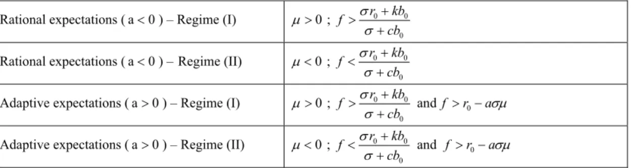
With rational expectations (a 0< ), the solution has a saddle-path structure. Two locally-stable regimes exist. First, an active monetary policy (µ >0) can be implemented as long as fiscal policy is passive (see table 1) and stabilises public debt. Second, if fiscal policy is active (f =0), monetary policy must be passive (µ <0) to stabilise debt. These regimes are exactly those found by Leeper (1991) within a neoclassical framework. The case with an active fiscal policy and a passive monetary policy is consistent with the FTPL. Stability conditions are very slightly dependent on the value of k (see table 1); and the FTPL can hold even if consumers are Ricardian (c k= =0).
Table 1: Stability conditions
Rational expectations ( a 0< ) – Regime (I) 0 0 0 0 ; f r kb cb σ µ σ + > > + Rational expectations ( a 0< ) –Regime (II) 0 0
0 0 ; f r kb cb σ µ σ + < < + Adaptive expectations ( a 0> ) – Regime (I) 0 0
0 0 ; f r kb cb σ µ σ + > > + andf > −r0 aσµ
Adaptive expectations ( a 0> ) – Regime (II) 0 0 0 0 ; f r kb cb σ µ σ + < < + and f > −r0 aσµ
Now, suppose that inflation is sluggish (a 0> ). The model is naturally stable if µ >0 and f is enough high. Combining an active monetary policy with a passive fiscal one ensures the stability of the model.
But a more fundamental question within this expectations regime is: can we still find a situation which illustrates the FTPL? The answer is no in the case in which fiscal policy does not respond to public debt growth. Indeed, if f = is coupled with 0 µ <0, the model is locally unstable since the trace of matrix A is always positive. The strict version of the FTPL is impossible in this framework.
Nonetheless, if one studies a smooth version of this theory (f >0 is coupled with µ <0), possible values for f which induce a stable economy require that:
(19) 2
0 0
This condition states that the net wealth effect must be strictly positive (remember that µ<0), otherwise the model with adaptive expectations is unstable. The existence of Ricardian consumers in this framework is thus a sufficient condition to reject the FTPL, contrary to the result of LWL.
The importance of parameter k in the stability of the model with adaptive expectations is best understood in comparison with the rational expectations framework with a passive central bank (µ < ). Within the latter model, after a negative public expenditure shock, the0 inflation rate immediately decreases, and then progressively returns to its initial steady state value. During this period, the real interest rate is higher and public debt is below its initial level. Introducing a net wealth effect (k>0) has only a marginal impact. With adaptive expectations, the shock-induced progressive decrease in the inflation rate provokes a progressive rise in the real interest rate; then, a persistent (or permanent) fall in the output, unless households have a wealth behaviour. With k>0, the rise in the real interest rate increases public debt and consumption, so that output recovers if the real wealth effect is tough enough (condition (19)). This process thus necessitates that the fiscal authorities do not limit too much the variations in the public debt to GDP ratio (f is not high).
If monetary policy is passive and prices expectations are adaptive, the minimum value for k obviously increases with the gap between the interest rate and the GDP growth rate and with the under-reaction of the central bank; and it decreases with the level of public debt.
In table 2, we used different values for parameters to assess the minimum value of parameter k given by eq. (19) and the possible range of values for the parameter f. Except for parameters a and σ , values were taken from Leith and Wren-Lewis.
First, for plausible values of the parameters (baseline case – the data period is annual), results show that the minimum value for the net wealth effect is equal to 23.2%. This is quite substantial, if one considers that empirical evidence on this net wealth effect generally gives small values (see Ludvigson and Steindel, 1999)5. Second, stable values for f are rare. Finally, in order to obtain empirically consistent values of k, we must suppose that monetary policy, though still under-reacting to inflation, reacts with more stringency towards this target: for instance, for µ = −0.1 (rather than µ = −0.5), k must be superior to 5.8%, and the necessary degree of stabilisation of public debt must be very small (between 5.5 et 6.5%),
otherwise the economy faces unstable dynamics. To obtain small minimum values for k, in a context of a very passive monetary policy, one can also use unrealistic small values for parameter a (Leith and Wren-Lewis, 2000), or for parameter σ (van Aarle and alii, 2001). Using the parameter set used for instance in Hughes Hallett and Vines (1993), the FTPL would lose any relevance with sluggish inflation.
Table 2: Alternative degrees of fiscal feedback
Baseline Variant LWL (2000) van Aarle and alii
(2001)
Hughes Hallett and Vines (1993) a 0.5 - 0.1 0.4 0.5 σ 0.5 - 0.65 0.2 1.25 µ -0.5 -0.1 -0.5/-0.1 -0.5 -0.5 k min 0.232 0.058 0.084/0.029 0.055 1.138 f min 0.155 0.055 0.063/0.037 0.07 0.343 f max 0.1652(1) 0.065(2) 0.141(2)/0.058 0.09(2) n.a. N.B.: b0=0.404;c=0.5;r0=0.03. (1): computed with k=0.25 (2): computed with k=0.075
The effects of a shock on public expenditures may usefully be illustrated by numerical simulations. Results are reported in the appendix. Public expenditures are increased by 0.5 point of GDP in the first year, and then linearly dies away6. Parameters are taken from the variant values in table 2. Parameter k is set at 0.075 and the response of taxes to public debt is supposed to be equal to its maximum possible value: 0.064. One can observe that the increase in public expenditures stimulates aggregate demand, temporarily increasing both inflation and output. The decrease in the real interest rate, due to a passive monetary policy, is rather inflationary. But it also reduces net interests paid on government debt, so that public debt is reduced and inflation goes back to its initial steady state level.
5 The estimated marginal propensity to consume out of wealth varies from 3.8% to 5%, depending on the methodology.
The situation is quite different if we use LWL’s parameter set (µ is set at –0.1). Although the effect of the shock on the output is more temporary, inflation persists longer than with baseline values. This is consistent with the low level of parameter a in the Phillips curve. The upper bound for f being lower than in the baseline (see table 2), the initial growth in public debt also dies away more slowly than in the variant case. The return path towards the new steady state values for the real interest rate and the tax rate is rather long, in comparison with the variant case.
V. Conclusion
The FTPL has now become a prominent theory of the determination of the price level. At its core, one finds the interactions of monetary and fiscal policies, and governments facing the possibility to act in a non-Ricardian manner, generally in a rational expectations framework. In the present paper, we have questioned the relevance of the FTPL in an adaptive expectations framework. More specifically, we have endeavoured to demonstrate to what extent the validity of the FTPL also depends on consumers being non-Ricardian.
Four main points have emerged. First, with prices driven by rational expectations, the qualitative results of the strategic interactions between monetary and fiscal policymakers do not depend on the Ricardian or non-Ricardian behaviour by the households: that k be nil or strictly positive modifies only marginally the stability conditions of the model used in section IV. Second, with sluggish inflation, the strong version of the FTPL does not bring to a dynamically stable economy. Unless governments react somewhat to the change in the public debt to GDP ratio, the FTPL is not valid. Third, a government reacting to public debt changes is not a sufficient condition for a weak version of the FTPL to hold. In this situation, stability conditions depend crucially on the existence and size of the wealth effect. If this wealth effect is too low (or too high) and monetary policy is passive, there is no existing degree of reaction of the government to debt variations which is sufficient to preserve the economy from unstable dynamics. Fourth, in the case of sluggish inflation, the FTPL is incompatible with Ricardian consumers. Hence, the compatibility of the FTPL with sluggish inflation appears very problematic.
References
AARLE B. (VAN), J.C. ENGWERDA, J.E.J. PLASMANS and A. WEEREN (2001),
“Macroeconomic Policy Interaction under EMU: A Dynamic Game Approach”, Open Economies Review, 12.
BARRO R.J. (1974), “Are Government Bonds Net Wealth ?”, Journal of Political
Economy, 82, November-December.
BENIGNO P. and J.D. LOPEZ-SALIDO (2001), “Inflation Persistence and Optimal Monetary
Policy in Europe”, mimeo, August.
BLANCHARD O.J. (1985), “Debt, Deficits, and Finite Horizons”, Journal of Political
Economy, 93(2), April.
BUITER W.H. (1998), “The Young Person’s Guide to Neutrality, Price Level
Indeterminacy, Interest Rate Pegs, and Fiscal Theories of the Price Level”, NBER Working Paper 6396, February.
BUITER W.H. (2000), “The Fiscal Theory of the Price Level: a Critique”, forthcoming in
the Economic Journal.
CALVO G.A. (1983), “Staggered Contracts in a Utility-Maximizing Framework”, Journal
of Monetary Economics, 12, September.
CLARIDA R., J. GALI and M. GERTLER (1998), “Monetary Policy Rules in Practice, some
international evidence”, European Economic Review, 42, April.
CLARIDA R., J. GALI and M. GERTLER (2000), “Monetary Policy Rules and
Macroeconomic Stability: Evidence and some Theory”, Quarterly Journal of Economics, 115(1), February.
COCHRANE J.H. (1998), « A Frictionless View of US Inflation», NBER Macroeconomics
Annual 1998, MIT Press.
FUHRER J.C. (1997), “The (Un)Importance of Forward-Looking Behavior in Price
Specifications”, Journal of Money, Credit, and Banking, 29(3), August.
GALI J., M. GERTLER and J.D. LOPEZ-SALIDO (2001), “European Inflation Dynamics”,
European Economic Review, 45(7), June.
HUGHES HALLETT A.J. and D. VINES (1993), “On the Possible Costs of European
Monetary Union”, The Manchester School, 61(1), March.
LEEPER E. (1991), “Equilibria under ‘Active’ and ‘Passive’ Monetary Policies”, Journal
of Monetary Economics, 27.
LEITH C. and S. WREN-LEWIS (2000), “Interactions between Monetary and Fiscal
Policies”, Economic Journal, Conference Papers, 110, March.
LUDVIGSON S. and C. STEINDEL (1999), “How Important is the Stock Market Effect on
Consumption?”, FRB of New York, Economic Policy Review, 5(2), July.
McCALLUM B.T. (1998), “Indeterminacy, Bubbles and the Fiscal Theory of Price Level
Determination”, NBER Working Paper 6456, March.
MANKIW N.G. (2001), “The Inexorable and Mysterious Trade-Off Between Inflation and
Unemployment”, Economic Journal, Conference Papers, 111(471), May.
SIMS C.A. (1994), “A Simple Model for the Determination of the Price Level and the
Interaction of Monetary and Fiscal Policy”, Economic Theory, 4.
WOODFORD M. (1995), “Price-Level Determinacy Without Control of a Monetary
Aggregate”, Carnegie-Rochester Conference Series on Public Policy, 43, December.
WOODFORD M. (1996), “Control of the Public Debt: a Requirement for Price Stability?”,
NBER. Working Paper n°5684, July.
WOODFORD M. (1998), “Public Debt and the Price Level”, mimeo, July.
WOODFORD M. (2001), “Fiscal Requirement for Price Stability”, Journal of Money,
Appendix
N.B.: f=0.064; k=0.075.