Conventions in the foreign exchange market : Can they really explain exchange rate dynamics ?

Conventions in the Foreign Exchange Market: Can they really explain Exchange Rate Dynamics?

Gabriele Di Filippo1

Department of Economics, LEDA-SDFi, University Paris IX Dauphine

First Version: October 2009 Revised Version: January 2011

Abstract

The present article provides an unorthodox model exchange rate dynamics based on conventions that prevail among market participants. We build a theoretical model that highlights the mechanisms underlying the formation of market conventions. We then test this model empirically on the euro/dollar exchange rate between January 1995 and December 2008. We rely on two alternative methods: a macroeconomic analysis and an econometric analysis based on the estimation of a time-varying parameter model. Both methods show that market switches between fundamentals considered in a bull convention and in a bear convention explain the euro/dollar dynamics between January 1995 and December 2008. Besides, at horizons longer than 1 month, the out-of-sample forecasting power of the convention model beats the traditional exchange rate models and the random walk.

Keywords: Exchange Rate Dynamics, Convention Theory, Imperfect Knowledge Economics,

Kalman filter, Genetic Algorithm

JEL Codes: G10, G12, F31

1

Author Contact: gabriele.di_filippo@yahoo.fr, gabriele.difilippo@daupine.fr; University Paris IX Dauphine, Office B313, Place du Maréchal de Lattre de Tassigny 75775 Paris CEDEX 16, France. For useful comments, I thank Giancarlo Gandolfo (Univ. La Sapienza), Frank Heinemann (Univ. of Technology, Berlin), Stephan Schulmeister (WIFO, Wien) and Henri Sterdyniak (OFCE, Paris). I am also grateful to the participants at the PhD seminars of the University Paris IX Dauphine (EDOCIF and CEREG), the 3rd FIW Conference in International Economics (Wien, Austria), the 2010 ADRES Doctoral Conference (Lyon, France) and the conference in Honor of Giancarlo Gandolfo on Advances in International Economics and Economic Dynamics (Università La Sapienza, Rome). I am also grateful to Sergio De Stefanis and Marcello d’Amato (Università di Salerno). All the remaining errors are of the author only.

1. Introduction

The present paper provides an unorthodox way to model exchange rate dynamics based on conventions that prevail among market participants. The intuition behind the convention model is based on a stylised fact highlighted by De Grauwe (2000). De Grauwe argues that agents tend to look for fundamentals that confirm the observed movements in the exchange rate. For instance, economists attibuted the large depreciation of the euro relative to the dollar between January 1999 and December 2002 to the strong growth performances in the United States relative to the euro zone. On the contrary, the appreciation of the euro relative to the dollar between December 2002 and December 2004 was justified by large current account deficits in the United States compared to the euro zone. Bachetta and Van Wincoop (2005) theorised this idea in the scapegoat model. A fundamental variable is taken as a scapegoat to explain the exchange rate dynamics in a given period of time. Our approach differs strongly from Bachetta and Van Wincoop (2005). Our convention model borrows more elements from the Imperfect Knowledge Economics (IKE) approach pioneered by Frydman and Goldberg (2007).

We first build a theoretical model to explain the mechanisms underlying the formation of market conventions. The simulated exchange rate from the theoretical convention model replicates several stylised facts highlighted empirically in the exchange rate dynamics. We then test this model empirically on the euro/dollar exchange rate. The period of analysis spans January 1995 to December 2008. We rely on two alternative methods. The first method is a macroeconomic analysis that aims at explaining the euro/dollar movements by relying on the consensus of economists. This method is based on the analysis of the fundmantals used by the economic and financial to justify the euro/dollar dynamics. The second method is based on an econometric approach. We estimate a time-varying parameter model to find the conventions that drive the euro/dollar dynamics.

Both methods show that market switches between fundamentals considered in a bull convention and in a bear convention explain the euro/dollar dynamics between January 1995 and December 2008. More precisely, the model shows that during the period of analysis, the market puts a large accent on the US and European productivity indices and dividend yields in times of optimism while a large weight is put on the US and European external debts, oil prices and US house prices in times of pessimism. The analysis underlines the existence of a non-linear relationship between fundamentals and the euro/dollar exchange rate. In other words, some fundamentals may be more important at some periods of time for the determination of exchange rate dynamics while other fundamentals are important at other periods of time.

Both methods identify three major conventions in the euro/dollar market. The first convention is the new economy convention that covered the period January 1995 - December 2000. Investors were relatively more optimistic in the growth perspectives of the US economy than in European economies. The dollar experiences a strong appreciating trend in this period. Between January 2001 and June 2003, the market relies on a bear convention based on the huge external debt of the US economy. The dollar starts a strong depreciating trend in this period. Then, between July 2003 and December 2005 two competing conventions prevailed in the market. A bear convention that focused mainly on the large US current account deficits; and a bull convention that pointed to the spectacular recovery of the US economy from the internet bubble burst. During this period the dollar alternates between short-lasting appreciating and depreciating trends according to whether the bull convention dominates the bear one. After January 2006, fundamentals worsened in the US economy. The bear convention started to dominate the bull one. The spark of the subprime crisis in June 2007 definitely led to the domination of the bear convention in the market.

The article compare thes predicitve performances of the convention model with regards to alternative models. Results show that at horizons longer than 1 month, the out-of-sample forecasting power of the convention model beats the ones of traditional models of exchange rate and of the random walk.

Section 2 presents the main pillars of convention theory and proposes a theoretical model that defines the mechanisms underlying the formation of market conventions. Sections 3 and 4 finds the possible conventions that prevailed for the euro/dollar exchange rate among market agents between January 1995 and December 2008. Section 3 identifies the conventions by relying on a macroeconomic analysis while section 4 rests on an econometric approach based on the estimation of a time-varying parameter model. Section 4 tests the out-of-sample predictive power of the convention model relative to alternative models. Section 5 concludes.

2. Theoretical concepts

2.1 The main principles of convention theory

Convention theory has been developed by the pioneered work of Lewis (1969), Sugden (1989) and Peyton Young (1996). Convention theory comes as an alternative to the traditional theory of asset pricing. Traditional models of asset pricing are based on the efficient market hypothesis (EMH) and the rational expectation hypothesis (REH). Such models assume objectivity ex ante of the future and the existence of a unique intrinsic asset value (the fundamental value). In the tradition of the Arrow-Debreu model, the REH states that a representative agent can predict the future value of an asset by associating ex ante predetermined probabilities to exogenous future events. A rational agent can hence assess the fundamental value of an asset by computing the expected returns of the asset in each state of the Nature conditional on the disposable stock of information. According to the EMH, every asset price has a unique fundamental value that includes all the relevant information of the asset.

Models based on the EMH and the REH offer poor empirical performances concerning the explanation and prediction of asset price dynamics, especially exchange rates (Meese and Rogoff (1983), Cheung, Chinn and Garcia Pascual (2005)). Such models led to unresolved asset pricing puzzles. Besides, assuming the existence of a unique fundamental value for an asset appears rather unrealistic. In a previous work, Bouveret and Di Filippo (2009) show that for the euro/dollar exchange rate, the market does not rely on a unique definition of the fundamental exchange rate but rather on a large panel of fundamental values. Each fundamental value belongs to a specific model designed by a particular agent. These facts cast doubts on the relevance of models based on the traditional asset pricing theory.

Convention theory adopts a rather opposite view to the traditional theory. Following Knight (1921) and Keynes (1936), convention theorists claim that the future is totally uncertain. No agent has the ability to know the probability distribution of future outcomes. The future is here shaped by the heterogeneity of opinions that agents frame on the fundamental value of an asset. There are as many fundamentals as there are opinions about the fundamental value of an asset. The future becomes hence subjective: each agent has his/her own opinion about the future value of the asset. All these opinions - translated into models of exchange rate determination - lead to the existence of multiple asset price equilibria in the market. The key question is how do these opinions converge towards a particular equilibrium? Individual opinions converge towards a particular equilibrium through a mimetic mechanism. This mechanism was early illustrated by Keynes (1936) in his beauty contest. The primary objective for an agent in the market is to anticipate the reaction of the majority of

participants in the market. As a matter of fact, if a market is bull on a given asset, an agent will have to buy the asset even if fundamentals tell him/her to sell the asset. This self-referential behaviour is rational at an individual level although it can lead to irrational phenomena (such as price bubbles) at a collective level. The self-referential behaviour consists in detecting striking events that could catch the attention of the majority of agents in the market. The choice of striking fundamentals is based on a trial-and-error strategy. Agents bet on the possible striking fundamentals that could catch the attention of the majority of agents in the market. Agents then build a model based on the selected fundamentals. The revisions of mistaken bets (or of bad models) imply an increasing volatility in asset prices. The market will stabilise itself when all agents - through mimetism - will focus on a particular striking set of fundamentals. At this point, agents have found a particular model based on a specific set of fundamentals. All agents in the market legitimate this model. This model is called a convention. A convention is therefore a fundamental model legitimated by all agents in the market, in a given time period. A convention therefore creates a focal point that helps resolving the problem of multiple asset price equilibria in the market. Once a convention is determined in the market, asset price volatility decreases. A convention therefore acts as a guide through the uncertainty concerning the future dynamics of asset prices. Indeed agents can rely on the convention to form their expectations on the future value of the asset.

A convention can thus be defined as a particular fundamental model adopted by the majority of agents in a market concerning the future economic perspectives (Orléan (2006)). A convention often ignores other fundamentals that go against it. In order to live long enough, the asset price dynamics fitted by the convention has to match the actual dynamics of asset prices. However, market agents will not abandon a convention at the first anomalies i.e. when the empirical dynamics of asset prices go against the ones assumed by the convention. Agents will do so when there will be a series of events that are in opposition to the fitted exchange rate provided by the current convention. Agents’ beliefs in the current convention vanish and the convention disappears from the market. The uncertainty on the future dynamics of asset prices increases and with it, exchange rate volatility. Market participants will then have to find a new convention.

2.2 A simple theoretical exchange rate model based on conventions

We set a simple theoretical model to explain the mechanisms underlying the formation of market conventions in the foreign exchange market. The model borrows elements from the Imperfect Knowledge Economics (IKE) approach by Frydman and Goldberg (2007).

We assume two countries (domestic and foreign) in an asymmetric world. The assumption of an asymmetric world implies that the influence of a given fundamental in the domestic and foreign countries does not have the same effect on exchange rate dynamics.

Following the IKE approach, the model considers two types of representative agents in the market: an optimistic (or bull) agent and a pessimistic (or bear) agent. The model is based on the following mechanism. When agents are relatively more optimistic in the domestic country than in the foreign country, they expect an appreciation of the domestic currency (and

vice versa). Conversely, when agents are more pessimistic in the domestic country than in the

foreign country, they anticipate a depreciation of the domestic currency (and vice versa). Agents are characterised by bounded rationality. Following a trial-and-error strategy, agents choose a bunch of fundamentals among the available set of fundamentals that best explain past exchange rate dynamics. We model the choice of fundamentals through a genetic algorithm2.

2

The first step of the genetic algorithm is the initialization of the variables. We assume a set of 8 pairs of fundamentals split into two subsets.

ΩBull = {(f1, f2*), (f3, f4*), (f5, f6*), (f7, f8*)}

ΩBear = {(f9, f10*), (f11, f12*), (f13, f14*), (f15, f16*)} (1)

The bull (bear) subset represents the stock of information used by optimistic (pessimistic) agents to forecast future exchange rate dynamics. As agents have bounded rationality, they rely on a particular stock of fundamentals to make their forecasts and ignore other fundamentals. In other words agents do not take account of the entire stock of information (ΩBull and ΩBear) but rely instead on a particular subset of information to make their forecasts (either ΩBull or ΩBear).

Agents are assumed to have knowledge of economic theory. In other words, they know the theoretical sign of the relationship between a given fundamental and the exchange rate. We assume that:

0 1 > t , t df ds ; 0 2 < * t , t df ds ; 0 3 > t , t df ds ; 0 4 < * t , t df ds ; 0 5 > t , t df ds ; 0 6 < * t , t df ds ; 0 7 > t , t df ds ; 0 8 < * t , t df ds (2a) 0 9 < t , t df ds ; 0 10 > * t , t df ds ; 0 11 < t , t df ds ; 0 12 > * t , t df ds 0 13 < t , t df ds ; 0 14 > * t , t df ds ; 0 15 < t , t df ds ; 0 16 > * t , t df ds (2b)

For example, if f1,t and f2,t are considered respectively as the domestic and foreign

interest rates, then an increase in the interest rate differential in favour of the domestic economy (d(f1,t – f2,t) > 0) will induce an appreciation of the domestic currency (dst > 0). Also,

if f9,t and f10,t are considered respectively as the domestic and foreign stocks of external debt,

then an increase in the stock of domestic debt other things being equal (d(f1,t – f2,t) > 0) leads

the domestic currency to depreciate (dst < 0).

Fundamentals are assumed to follow a random walk: k t k t k t f f = ₋₁ +ε (3) Where k t

ε mimics the impact of news on the fundamentals k t

ε → iidN(0,σεk) The second step of the genetic algorithm is the selection of the variables. As agents cannot take account of all fundamentals due to bounded rationality, they select a limited bunch of fundamentals. We assume that in a given state, agents select two pairs of fundamentals among the four pairs available in a given state. Thus, agents include four fundamentals (either from ΩBull or from ΩBear) in their model.

The selection of fundamentals that in turn creates a model of exchange rate determination is based on a fitness process. Agents first test the in-sample historical explanatory power of each possible model based on the above pairs of fundamentals. They then select the model (or the fundamentals) that best explain past exchange rate dynamics.

Thus, each category of agents (optimistic or pessimistic) tests 6 possible models. We therefore end up with 12 models.

Bull agents test the following models (bull models are indexed from 1 to 6): * t , l t , l t , l t , l * t , k t , k t , k t , k t , i t f f f f s =β₀ +β −β ₊₁ +β −β_{+1 +1} With k ≠ l (4a) Where k =2a+1 and l = 2a (a = 0 to 4); i = 1 to 6; β is a constant 0_,t

Bear agents tests the following models (bear models are indexed from 7 to 12): * t , n t , n t , n t , n * t , m t , m t , m t , m t , j t f f f f s =β₀ +β −β _{+1 +1} +β −β _{+1 +1} With m ≠ n (4b) Where m =2b+1 and n = 2b (b = 5 to 8); j = 7 to 12; β is a constant 0_,t

In order to assess the fitness of the above models, each agent estimates the models by ordinary least squares (OLS). The aim is to find the coefficients β that minimize the sum of squared residuals of the model:

∑

β

β

β

The estimated coefficients are given by:

∑

∑

The fitted exchange rate is defined by:

∑

∑

∑

Each agent computes the in-sample mean squared error (MSE) based on the past exchange rate dynamics:

2 1 1 ) sˆ s ( n MSE _{t h} n t h h t h t − = −

∑

The selected models satisfy the following conditions:

{

}

{

}

The expected exchange rate from the model used by each agent is defined as:

* t , l t , l t , l t , l * t , k t , k t , k t , k t , i 1 t t o,(s ) ˆ ˆ f ˆ f ˆ f ˆ f E ₊ =

β

β

β

β

β

β

β

β

β

β

The third step of the genetic algorithm is the reproduction of the best model. Agents drop the fundamental variables that do not explain well the dynamics of exchange rate and look for the ones that provide a better fit of past exchange rate dynamics. In other words, agents re-iterate the procedure described above.

We assume that the proportion of optimistic and pessimistic agents in the market varies trough time. We define the proportion of optimistic and pessimistic agents in the market as: )] exp( ) [exp( ) exp( ' t , p ' t, o ' t , o t , o

γπ

γπ

γπ

ω

γπ

γπ

γπ

ω

Where ωo,t + ωp,t = 1 and 0 < γ < 1

The parameter γ represents the intensity at which agents revise their forecasting rules. Usually, we set γ close to zero and away from unity since as underlined in section 2.1, a convention does not disappear at the first anomalies between the fitted asset price dynamics by the convention and the actual asset price dynamics.

The profitability π'i,t of each rule is evaluated according to the profit πi,t and the risk

σ²i,t related to this rule:

π'i,t = π i,t - µσ²i,t i = o, p (12)

The parameter µ represents the coefficient of risk aversion. The risk associated to a forecasting rule is defined as the variance of the forecasting error:

σ²i,t = [Eit-1(st) - st]² i = o, p (13)

The profit π i,t related to a forecasting strategy is defined as the one-period earnings of

investing one unit of domestic currency in the foreign asset:

Where      < = = = > = 0 x if 1 -sgn[x] 0 x if 0 sgn[x] 0 x if 1 sgn[x]

We obtain the expected exchange rate at time t+1 by aggregating agents’ forecasts in the market:

Et(∆st+1) = ωo,tEo,t(∆st+1) + ωp,tEp,t(∆st+1) (15)

Hence: ∆st+1Market = - ωo,t∆st+1Bull+ ωp,t ∆st+1Bear + εt+1 (16)

Figure 1.1 shows the simulations results of the theoretical convention model for 1000 periods (we assume µ = 5 and γ = 0,2). The blue margins mean that the market is in majority optimistic (P(St=Bull/It) > 0,5) while the white margins mean that the market is globally

pessimistic (P(St=Bull/It) < 0,5).

Figure 1.1: Simulated exchange rate dynamics and probability to be in the bull state

0 0,5 1 1,5 2 2,5 3 3,5 4 -10 -5 0 5 10 15 20 25 30 1 3 6 7 1 1 0 6 1 4 1 1 7 6 2 1 1 2 4 6 2 8 1 3 1 6 3 5 1 3 8 6 4 2 1 4 5 6 4 9 1 5 2 6 5 6 1 5 9 6 6 3 1 6 6 6 7 0 1 7 3 6 7 7 1 8 0 6 8 4 1 8 7 6 9 1 1 9 4 6 9 8 1

NB: The black lines represents the market exchange rate (left scale) ; the blue line represents the probability to be in the bull state (right scale); the orange line represents the Hodrick-Prescott filter (λ = 14400) of the probability to be in the bull state (right scale).

Figure 1.1 shows that the simulated exchange rate alternates between periods of appreciating and depreciating trends. Also, the proportion of bull and bear agents in the market varies through time.

In this model, agents go through two selection processes that define two switching mechanisms.

The first selection process (equations (1) to (10b)) is the selection of the best model by bull and bear agents. This choice is based on the relative performances of the past explanatory powers of exchange rate models based on fundamentals coming respectively from the bull and bear information stocks. Through time, bull and bear agents switch between their respective models and choose the model that provides the best explanatory power of past exchange rate dynamics. Figure 1.2 represents the models chosen by optimistic and pessimistic agents through time.

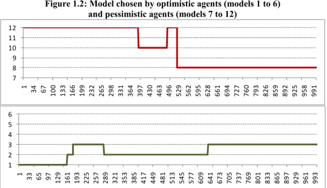
Figure 1.2: Model chosen by optimistic agents (models 1 to 6) and pessimistic agents (models 7 to 12)

7 8 9 10 11 12 1 3 4 6 7 1 0 0 1 3 3 1 6 6 1 9 9 2 3 2 2 6 5 2 9 8 3 3 1 3 6 4 3 9 7 4 3 0 4 6 3 4 9 6 5 2 9 5 6 2 5 9 5 6 2 8 6 6 1 6 9 4 7 2 7 7 6 0 7 9 3 8 2 6 8 5 9 8 9 2 9 2 5 9 5 8 9 9 1 1 2 3 4 5 6 1 3 3 6 5 9 7 1 2 9 1 6 1 1 9 3 2 2 5 2 5 7 2 8 9 3 2 1 3 5 3 3 8 5 4 1 7 4 4 9 4 8 1 5 1 3 5 4 5 5 7 7 6 0 9 6 4 1 6 7 3 7 0 5 7 3 7 7 6 9 8 0 1 8 3 3 8 6 5 8 9 7 9 2 9 9 6 1 9 9 3

NB: The upper figure represents the model chosen by pessimistic agents (models 7 to 12); the lower figure represents the model chosen by optimistic agents (models 1 to 6). The left scale represents the models chosen; the horizontal scale represents the time period.

Figure 1.2 shows that between t = 1 and t = 300 optimistic agents alternate between model 1, 2 and 3. Over the same period, pessimistic agents rely on model 12. Thus in this period, model 12 provides the best explanatory power of past exchange rate dynamics given the stock of fundamentals used by bear agents.

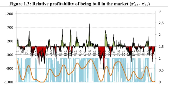
The second selection process (equations (11) to (14)) is the choice of whether being bull or bear in the market. This choice depends on the relative profitability of the selected bull model relative to the selected bear model. Through time, agents can switch between being a bull or a bear agent given the profitability of the model selected by bull and bear agents. Figure 1.3 represents the relative profitability of being bull in the market (π'o,t - π'p,t). The

green area means that the selected bull model generates a positive profitability relative to the selected bear model. Conversely, the red area means that being bull is less profitable than being bear.

Figure 1.3: Relative profitability of being bull in the market (π'o,t - π'p,t) 0 0,5 1 1,5 2 2,5 3 -1300 -800 -300 200 700 1200 1 3 6 7 1 1 0 6 1 4 1 1 7 6 2 1 1 2 4 6 2 8 1 3 1 6 3 5 1 3 8 6 4 2 1 4 5 6 4 9 1 5 2 6 5 6 1 5 9 6 6 3 1 6 6 6 7 0 1 7 3 6 7 7 1 8 0 6 8 4 1 8 7 6 9 1 1 9 4 6 9 8 1

NB: The black lines represents the difference between the profitability of the selected bull model and the profitability of the selected bear model (left scale) ; the blue line represents the probability to be in the bull state (right scale) ; the orange line represents the Hodrick-Prescott filter (λ = 14400) of the probability to be in the bull state (right scale).

Figure 1.3 shows that when the selected model by bull agents generates a positive profitability relatively to the selected bear model, bull agents dominate the market. On the contrary, when the selected model by bull agents generates a negative profitability relatively to the selected bear model, bear agents become dominant in the market.

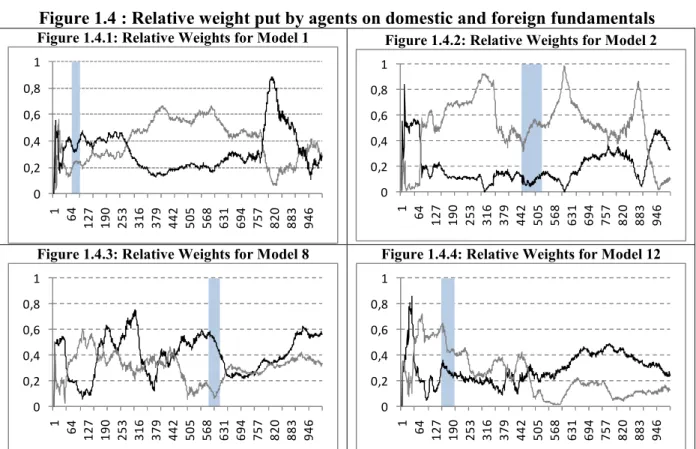
Figure 1.4 shows the relative weights put by agents on domestic and foreign fundamentals for model 1, model 2, model 8 and model 12. These relative weights put by agents on domestic and foreign fundamentals are computed as the contributions of the coefficients for the estimated models in the bull state (ΩBull_Model1) and in the bear state (

Bear Model1

Ω ).

For example, in the case of model 1, we have:

' Bull Model f ˆ f ˆ f ˆ f ˆ f ˆ f ˆ 4 3 3 2 2 1 1 3 3 1 1 1

β

β

β

β

β

β

β

β

β

β

β

β

Figure 1.4 : Relative weight put by agents on domestic and foreign fundamentals Figure 1.4.1: Relative Weights for Model 1

0 0,2 0,4 0,6 0,8 1 1 6 4 1 2 7 1 9 0 2 5 3 3 1 6 3 7 9 4 4 2 5 0 5 5 6 8 6 3 1 6 9 4 7 5 7 8 2 0 8 8 3 9 4 6

Figure 1.4.2: Relative Weights for Model 2

0 0,2 0,4 0,6 0,8 1 1 6 4 1 2 7 1 9 0 2 5 3 3 1 6 3 7 9 4 4 2 5 0 5 5 6 8 6 3 1 6 9 4 7 5 7 8 2 0 8 8 3 9 4 6

Figure 1.4.3: Relative Weights for Model 8

0 0,2 0,4 0,6 0,8 1 1 6 4 1 2 7 1 9 0 2 5 3 3 1 6 3 7 9 4 4 2 5 0 5 5 6 8 6 3 1 6 9 4 7 5 7 8 2 0 8 8 3 9 4 6

Figure 1.4.4: Relative Weights for Model 12

0 0,2 0,4 0,6 0,8 1 1 6 4 1 2 7 1 9 0 2 5 3 3 1 6 3 7 9 4 4 2 5 0 5 5 6 8 6 3 1 6 9 4 7 5 7 8 2 0 8 8 3 9 4 6

NB: The black (grey) line represents the weight attributed to domestic (foreign) fundamentals.

The paragraph below provide a key understanding of the results from figures 1.1, 1.2, 1.3 and 1.4. We have here four cases in the market.

First, in figure 1.1, an appreciation (a depreciation) of the domestic (foreign) currency in the bull state means that agents are relatively more optimistic in the domestic economy than in the foreign economy. For example, in figure 1.1, from t = 70 to 100, the market is bull (P(St=Bull/It) > 0,5) and the domestic currency appreciates. Agents are in majority bull

because being bull is more profitable than being bear (figure 1.3). Optimistic agents rely on model 1 in this period (figure 1.2) and put more weight on domestic fundamentals than on foreign fundamentals (figure 1.4.1).

Secondly, in figure 1.1, an appreciation (a depreciation) of the foreign (domestic) currency in the bull state means that agents are relatively more optimistic in the foreign economy than in the domestic economy. For instance, in figure 1.1, from t = 450 to 525, the market is bull and the domestic currency depreciates. Figure 1.3 shows that over the period the profitability of being bull is higher than the one of being bear. The best model selected by bull agents in this period is model 2 (figure 1.2). Based on model 2, bull agents put more weight on foreign fundamentals than on domestic fundamentals (figure 1.4.2).

Thirdly, in figure 1.1, a depreciation (an appreciation) of the domestic (foreign) currency in the bear state means that agents are relatively more pessimistic in the domestic economy than in the foreign economy. As a matter of facts, from t = 580 to 620 in figure 1.1, the market is bear (P(St=Bull/It) < 0,5) and the domestic currency depreciates over the period.

The profitability of being bear is higher than the one of being bull (figure 1.3). The selected model by bear agents is model 8 (figure 1.2). Model 8 puts more weight on domestic fundamentals than on foreign fundamentals (figure 1.4.3).

Fourthly, in figure 1.1, a depreciation (an appreciation) of the foreign (domestic) currency in the bear state means that agents are relatively more pessimistic in the foreign economy than in the domestic economy. For instance, we observe in figure 1 from t = 150 to

200 that the market is bear and that the domestic currency appreciates. Being bear is indeed more profitable than being bull in this period (figure 1.3). The model chosen by bear agents is model 12 (figure 1.2). Model 12 puts a lower weight on domestic fundamentals than on foreign fundamentals (figure 1.4.4).

Finally, the theoretical convention model shows that exchange rate dynamics are driven by the time-varying fundamental models or equivalently by the convention models selected by market agents.

The convention model offers several advantages compared to recent models of exchange rate such as the heterogeneous agents models (De Grauwe and Grimaldi (2007)). Heterogeneous agents models explain exchange rates dynamics based on the behaviour of fundamentalist and chartist agents. Such models fully predetermine the behaviour of economic agents by associating an exogenous rule to each agent. Agents therefore act as robots in these models. On the contrary, the convention model follows the IKE approach by partially predetermining the behaviour of agents. Indeed, agents can use whatever rules or investment strategies. Such rules are allowed to evolve over time based on a trial-and-error strategy. Moreover, the convention model does not rely on the controversial definition of a fundamental exchange rate. On the contrary, heterogeneous agents models have to specify an arbitrary value for the fundamental exchange rate in the fundamentalist rule.

Having highlighted the mechanisms behind the formation of market conventions, we now test the theory of conventions in the foreign exchange market. The asset of interest is the euro/dollar exchange rate. The period of analysis runs from January 1995 to December 2008.

We rely on two methds to identify the fundamentals considered in conventions by market agents. The first method is a macroeconomic analysis. This method analyses the weight given to a particular fundamental by the economic and financial literature in a given period of time. The results are presented in section 3. The second method relies on the estimation of a time-varying parameter model. This method computes the time-varying dynamics of the coefficients value associated to a particular fundamental through time. The results are presented in section 4.

3. A macroeconomic analysis of market conventions

This section highlights the conventions that prevail in the euro/dollar market by relying on a macroeconomic analysis. The aim is to rely on the consensus of the market concerning the fundamentals that explains the euro/dollar movements. We rely on major articles from financial journals (Wall Street Journal and The Economist) as well as academic ones. We justify each argument by using figures from Thomson Datastream and from the Bureau of Economic Analysis3. The results of this analysis are organised in the following five sections.

3.1 January 1995 - December 2000: the internet convention or the superiority of the US economy compared to the euro zone

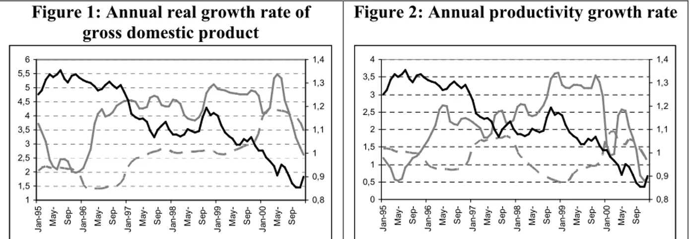
In the second half of the 1990s, the US economy experienced a stronger growth rate than Europe (an average of 8,3 % for the United States versus 5 % for Europe (figure 1)). Stronger growth in the United States was attributed to larger investments in new technologies compared to Europe. Such investments helped increase the productivity differential in favour

3

For figures 1 to 23, data comes from Thomson Datastream and the Bureau of Economic Analysis concerning capitals flows (figures 3, 7 and 21).

of the United States (figure 2). In December 2008, the differential in productivity growth rates amounted to 3 %. Numerous economists praised the glorious perspectives offered by the US economy. Some economists (of whom Jeremy Rifkin) even claimed that the US economy had reached a higher structural growth rate. The market was clearly in presence of a convention defining the US economy as more profitable than the European economy.

Figure 1: Annual real growth rate of gross domestic product

1 1,5 2 2,5 3 3,5 4 4,5 5 5,5 6 J a n -9 5 M a y -S e p -J a n -9 6 M a y -S e p -J a n -9 7 M a y -S e p -J a n -9 8 M a y -S e p -J a n -9 9 M a y -S e p -J a n -0 0 M a y -S e p - 0,8 0,9 1 1,1 1,2 1,3 1,4

Figure 2: Annual productivity growth rate

0 0,5 1 1,5 2 2,5 3 3,5 4 J a n -9 5 M a y -S e p -J a n -9 6 M a y -S e p -J a n -9 7 M a y -S e p -J a n -9 8 M a y -S e p -J a n -9 9 M a y -S e p -J a n -0 0 M a y -S e p - 0,8 0,9 1 1,1 1,2 1,3 1,4

NB: The dashed grey line refers to the euro zone; the solid grey line refers to the United States and the solid black line represents the euro/dollar nominal exchange rate.

Financial investors therefore expected higher returns in US stocks than in European stocks. They invested massively in US stocks, especially in companies belonging to the sector of the new economy (the ever-known start-ups). Net equity flows in the United States increased by an average of 24 % a year between 1998 and 2000 (figure 3). The annual average growth rate of the S&P500 between January 1995 and December 2000 amounted to 21 % a year (figure 23).

The birth of the euro zone in 1999 and the youth of the European Central Bank (ECB) - which had to set its credibility among market agents - led investors to be more timorous in the European economy than in the US economy.

Figure 3: Net equity flows in the United States (in millions of dollars)

-600000 -400000 -200000 0 200000 400000 600000 800000 1995 1996 1997 1998 1999 2000

Figure 4: Short run (3 months) interest rate 2 3 4 5 6 7 8 J a n -9 5 M a y -S e p -J a n -9 6 M a y -S e p -J a n -9 7 M a y -S e p -J a n -9 8 M a y -S e p -J a n -9 9 M a y -S e p -J a n -0 0 M a y -S e p - 0,8 0,9 1 1,1 1,2 1,3 1,4

NB: For Figure 3, the dark grey represents the US current balance; the light grey represents net flows of investment in Treasury bills and government bonds; the black represents net flows of investment in equity and foreign direct investment. For Figure 4, the dashed grey line refers to the euro zone; the solid grey line refers to the United States and the solid black line represents the euro/dollar nominal exchange rate.

The net inflow of capitals in the United States led to an appreciation of the dollar against the euro between January 2001 and December 2000. This appreciation was also induced by an interest rate differential in favour of the United States.

Therefore, between January 1995 and December 2000, markets were relatively more optimistic on the perspectives of the US economy relative to the ones of the European economy. The bull sentiment that prevailed in the market was referred to as the new economy convention or the internet convention.

3.2 January 2001-June 2003: the burst of the internet bubble and the end of the new economy convention

The over-optimistic sentiment in the US economy led to a bubble in stock prices: the internet bubble. This bubble burst in January 2001. This exogenous shock put an end to the new economy convention. Investors realised that their expectations on the perspectives of the US economy were too optimistic.

Financial papers began to put the accent on variables hidden during the internet convention. Stronger US growth rate was gauged on a growing debt of the public and the private sectors. US companies over-estimated the future demand and faced higher debt and excess capacities. The high level of US consumption rested on an increasing debt allowed by the positive wealth effect induced by the rise in stock prices.

The increase in public and private debt induced mechanically an increase in the deficit of the current account balance (figure 6) and induced the return of the twin deficits. A lot of economists began to ask about the sustainability of US deficits (Mann (2002)) and a possible fall in the dollar.

To counter the economic slowdown induced by the internet bubble burst, the Federal Reserve decreased dramatically its rates of interest. The interest rate differential became now in favour of the European economy (figure 5).

Figure 5: Short run (3 month) interest rate

0 1 2 3 4 5 6 7 8 J a n -9 5 J u l-9 5 J a n -9 6 J u l-9 6 J a n -9 7 J u l-9 7 J a n -9 8 J u l-9 8 J a n -9 9 J u l-9 9 J a n -0 0 J u l-0 0 J a n -0 1 J u l-0 1 J a n -0 2 J u l-0 2 J a n -0 3 J u l-0 3 0,8 0,9 1 1,1 1,2 1,3 1,4

Figure 6: Current balances over GDP

-5 -4 -3 -2 -1 0 1 2 1995 1996 1997 1998 1999 2000 2001 2002 2003 0,8 0,9 1 1,1 1,2 1,3 1,4

NB: For Figure 5, the dashed grey line refers to the euro zone; the solid grey line refers to the United States and the solid black line represents the euro/dollar nominal exchange rate. For Figure 6, the dark grey represents the US current balance and the light grey represents the European current balance.

Investors became thus relatively less confident in the US economy than in the European economy. They reduced investments in stocks and foreign direct investment (FDI) in the United States. Between January 2001 and June 2003, the S&P500 lost 44 % and the Eurostoxx 60 %. The financial scandals of Enron and Worldcom and then the attacks of the 11th September 2001 kept increasing the bear sentiment on the US economy. Equity flows in the United States decreased (figure 7) and the dollar stopped its appreciating trend begun earlier in January 1995 (figure 8). The dollar started to depreciate in June 2002. This depreciation was however contained by interventions of East-Asian central banks. Such agents bought US bonds to prevent a severe appreciation of their currency against the dollar.

The bear sentiment of investors on the US economy does not mean that investors became bull in the European economy. Indeed, the excess in the current balance experienced by the euro zone at that period (figure 6) suggests that the growth rate has been very low and is still very low in the euro zone during this period.

Figure 7: Net equity flows and net bond flows in the US (in millions of dollars)

-600000 -400000 -200000 0 200000 400000 600000 800000 1995 1996 1997 1998 1999 2000 2001 2002 2003

Figure 8 : Annual real growth rate of gross domestic product 0 1 2 3 4 5 6 J a n -9 5 J u n -9 5 N o v -9 5 A p r-9 6 S e p -9 6 F e b -9 7 J u l-9 7 D e c -9 7 M a y -9 8 O c t-9 8 M a r-9 9 A u g -9 9 J a n -0 0 J u n -0 0 N o v -0 0 A p r-0 1 S e p -0 1 F e b -0 2 J u l-0 2 D e c -0 2 M a y -0 3 0,8 0,9 1 1,1 1,2 1,3 1,4

NB: For Figure 7, the dark grey represents the US current balance; the clear grey represents net flows of investment in Treasury bills and government bonds; the black represents net flows of investment in equity and foreign direct investment. For Figure 8, the dashed grey line refers to the euro zone; the solid grey line refers to the United States and the solid black line represents the euro/dollar nominal exchange rate.

As a result, between January 2001 and June 2003, financial markets faced an increase in uncertainty concerning economic recovery either in the Euro zone or in the United States. Deflation fears induced by lower growth rates prevailed among economists and central bankers. The market definitely abandoned the internet convention. Agents became bear either in the United States and or in the euro zone. The bear sentiment was however relatively stronger in the United States than in the euro zone.

3.3 July 2003-December 2005: The birth of two competing conventions: the US consumption as the engine of the world economy versus the US as a net debtor

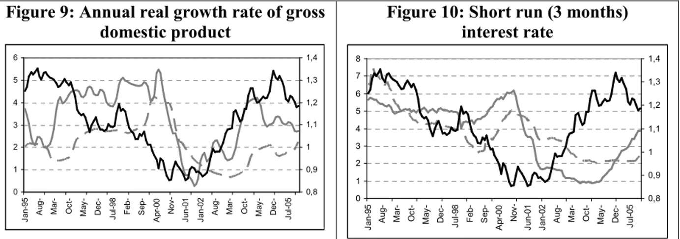
From July 2003, fears of deflation induced by the bubble burst vanished. The US economy was recovering surprisingly fast from the burst of the internet bubble (figure 9). Factors behind the US recovery were the large decrease of interest rates by the Federal Reserve (figure 10) coupled with an increase in public spending (through the decrease in taxes under the Bush government and the increase in military spending (related to wars in Iraq and in Afghanistan)).

Conversely, the Euro area was dealing with a weaker growth rate. Economists started to ask about the relevance of the institutional structure of the euro zone. They began to blame the Growth and Stability Pact because it could prevent the euro area from higher growth rates. Members of the euro zone seemed unable to lead a relevant fiscal policy to counter the economic slowdown. Between July 2003 and December 2005 the annual growth rate reached 1,7 % in the euro zone compared to 4,8 % in the United States (figure 9). Lower interest rates associated to surging house prices (figure 13) allowed US households to ease their access on credit and to increase their consumption. At that time, financial papers argued that the US consumption was the engine of the world economy.

Figure 9: Annual real growth rate of gross domestic product 0 1 2 3 4 5 6 J a n -9 5 A u g -M a r-O c t-M a y -D e c -J u l-9 8 F e b -S e p -A p r-0 0 N o v -J u n -0 1 J a n -0 2 A u g -M a r-O c t-M a y -D e c -J u l-0 5 0,8 0,9 1 1,1 1,2 1,3 1,4

Figure 10: Short run (3 months) interest rate 0 1 2 3 4 5 6 7 8 J a n -9 5 A u g -M a r-O c t-M a y -D e c -J u l-9 8 F e b -S e p -A p r-0 0 N o v -J u n -0 1 J a n -0 2 A u g -M a r-O c t-M a y -D e c -J u l-0 5 0,8 0,9 1 1,1 1,2 1,3 1,4

NB: The dashed grey line refers to the euro zone; the solid grey line refers to the United States and the solid black line represents the euro/dollar nominal exchange rate.

However, several factors seemed to limit investors’ confidence in the US economy. Indeed, the US consumption was gauged on a higher level of debt for US households. Besides, the return of growth in the United States generated no increase in employment. As shown in figure 11, the growth rate of employment was close to the one in the Euro zone although the growth differential was strongly in favour of the United States (figure 9). This fact was partly explained by relocations of US firms to China. Such relocations led the US economy to increase imports of Chinese goods which contributed to increase the US deficit (figure 12). In 2005, the US current deficit reached 6 % of GDP.

All these factors can explain why the dollar still depreciates even after the recovery of the US economy between July 2003 and December 2004.

Figure 11: Employment growth rate

-3 -2 -1 0 1 2 3 4 J a n -9 5 A u g -M a r-O c t-M a y -D e c -J ul -9 8 F e b -S e p -A p r-0 0 N o v -J u n -0 1 J a n -0 2 A u g -M a r-O c t-M a y -D e c -J ul -0 5 0,8 0,9 1 1,1 1,2 1,3 1,4

Figure 12: Current balance over GDP

-7 -6 -5 -4 -3 -2 -1 0 1 2 1995 1996 1997 1998 1999 2000 2001 2002 2003 2004 2005 0,8 0,9 1 1,1 1,2 1,3 1,4

NB: For Figure 11, the dashed grey line refers to the euro zone; the solid grey line refers to the United States and the solid black line represents the euro/dollar nominal exchange rate. For Figure 12, the dark grey represents the US current balance and the light grey represents the European current balance.

At the beginning of 2004, higher growth in the US and increasing oil prices led the Federal Reserve to increase its rates of interest (figure 10). The interest rate differential became in favour of the US economy in December 2004.

Finally, between July 2003 and December 2005, two competing conventions appeared in the market. A first convention (bear convention) focused mainly on large US current deficits and expected a fall in the dollar. A second convention (bull convention) pointed to the fast recovery of the US economy after the bubble burst and its good resistance relative to the increase in oil prices (figure 14). The bull sentiment was also attributed to the success of the fine monetary policy by Alan Greenspan, chairman of the Federal Reserve at that time. The

domination of the bear convention may explain the depreciation of the dollar between July 2003 and December 2004. Conversely, the domination of the bull convention may explain the appreciation of the dollar between January 2005 and December 2005.

3.4 January 2006 - June 2007: the weakening of the bull convention

Between January 2006 and June 2007, the bull sentiment associated to the resistance and the high potential of the US economy became more and more threatened by several negative news about the US economy.

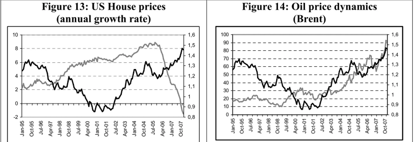
Indeed, the sustained growth in the United States between July 2003 and December 2005 was gauged on a positive growth rate of house prices. Between January 2006 and September 2007, the growth rate of US house prices decreased (figure 13). Economists began to warn about a possible burst of a bubble in US house prices.

On the other hand, oil prices were surging and acted as a burden on the budget of US households. The barrel of Brent reached 96,05 $ in November 2007 (figure 14). Investors feared a decrease in US households’ consumption either by the decrease in house prices that could close access to credit for US households or by the increase in oil prices that would reduce the disposable income of US households. Fears were also accentuated by the increase in interest rates by the Federal Reserve (figure 18) which raised the burden of debt for US households.

Figure 13: US House prices (annual growth rate)

-2 0 2 4 6 8 10 J a n -9 5 O c t-9 5 J u l-9 6 A p r-9 7 J a n -9 8 O c t-9 8 J u l-9 9 A p r-0 0 J a n -0 1 O c t-0 1 J u l-0 2 A p r-0 3 J a n -0 4 O c t-0 4 J u l-0 5 A p r-0 6 J a n -0 7 O c t-0 7 0,8 0,9 1 1,1 1,2 1,3 1,4 1,5 1,6

Figure 14: Oil price dynamics (Brent) 0 10 20 30 40 50 60 70 80 90 100 J a n -9 5 O c t-9 5 J u l-9 6 A p r-9 7 J a n -9 8 O c t-9 8 J u l-9 9 A p r-0 0 J a n -0 1 O c t-0 1 J u l-0 2 A p r-0 3 J a n -0 4 O c t-0 4 J u l-0 5 A p r-0 6 J a n -0 7 O c t-0 7 0,8 0,9 1 1,1 1,2 1,3 1,4 1,5 1,6

NB: For Figure 13 and 14, the solid black line represents the euro/dollar nominal exchange rate.

Negative news about the US economy were also illustrated by the worrying concerns about the sustainability of the US debt. US current deficits were evaluated at more than 6 % of US GDP in 2006 and about 5,5 % of US GDP in 2007 (figure 15). Fears increased among investors about a possible fall in the dollar and hence in the value of assets denominated in dollars. Threats by Chinese authorities to convert part of their huge stock of accumulated dollars (figure 16) in another currency accentuated fears by investors about a possible dollar fall.

Figure 15: Current balance over GDP -7 -6 -5 -4 -3 -2 -1 0 1 2 1995 1996 1997 1998 1999 2000 2001 2002 2003 2004 2005 2006 2007 0,8 0,9 1 1,1 1,2 1,3 1,4

Figure 16: Chinese dollar reserves (in millions of dollars)

0 200000 400000 600000 800000 1000000 1200000 1400000 1600000 1800000 J a n -9 5 O c t-9 5 J u l-9 6 A p r-9 7 J a n -9 8 O c t-9 8 J u l-9 9 A p r-0 0 J a n -0 1 O c t-0 1 J u l-0 2 A p r-0 3 J a n -0 4 O c t-0 4 J u l-0 5 A p r-0 6 J a n -0 7 O c t-0 7 0,8 0,9 1 1,1 1,2 1,3 1,4 1,5 1,6

NB: For Figure 15, the dark grey represents the US current balance and the light grey represents the European current balance. For Figure 16, the solid grey line refers to Chinese reserves and the solid black line represents the euro/dollar nominal exchange rate.

The rising bear sentiment in the US economy led investors to be relatively more optimistic on the perspectives of the euro zone. Investors became aware that the US economy had not significantly outperformed the European economy in the recent years. Growth in the Euro area was at its fastest pace since January 2002 and the growth differential between the United States and the euro zone became very thin from January 2007 to December 2007 (figure 17). In 2007, inflation fears related to the increase in oil prices led the ECB to increase its interest rates. At the end of 2007 the interest rate differential became in favour of the euro zone (figure 18).

Figure 17: Annual real growth rate of gross domestic product

0 1 2 3 4 5 6 J a n -9 5 O c t-9 5 J u l-9 6 A p r-9 7 J a n -9 8 O c t-9 8 J u l-9 9 A p r-0 0 J a n -0 1 O c t-0 1 J u l-0 2 A p r-0 3 J a n -0 4 O c t-0 4 J u l-0 5 A p r-0 6 J a n -0 7 O c t-0 7 0,8 0,9 1 1,1 1,2 1,3 1,4 1,5 1,6

Figure 18: Short run (3 month) interest rates 0 1 2 3 4 5 6 7 8 J a n -9 5 O c t-9 5 J u l-9 6 A p r-9 7 J a n -9 8 O c t-9 8 J u l-9 9 A p r-0 0 J a n -0 1 O c t-0 1 J u l-0 2 A p r-0 3 J a n -0 4 O c t-0 4 J u l-0 5 A p r-0 6 J a n -0 7 O c t-0 7 0,8 0,9 1 1,1 1,2 1,3 1,4 1,5 1,6

NB: The dashed grey line refers to the euro zone; the solid grey line refers to the United States and the solid black line represents the euro/dollar nominal exchange rate.

In December 2007, investors became uncertain about the perspectives offered by the US economy. Economists and central bankers began questioning whether the US economy would experience a soft-landing or a hard-landing. The bull convention that appeared between July 2003 and December 2005 in the United States was fading out at an increasing pace. The increasing domination of the bear convention may explain why the dollar depreciates between January 2006 and December 2007.

3.5 June 2007 - December 2008: The subprime crisis and the end of the bull convention in the US economy

The bankruptcy of two investment funds of Bear Stearns in June 2007 sparked a major financial crisis in the United States. In spring 2007, the Federal Reserve along with the ECB intervened massively in the interbank market to prevent a liquidity crisis.

The Federal Reserve began to decrease its interest rates in June 2007 (figure 20) while the ECB kept its rates unchanged because of inflation fears caused by increasing oil prices and also because growth forecasts were still more optimistic in the euro zone than in the United States (figure 19).

In October 2007, the bubble on US house prices burst (figure 13). Investors faced a great uncertainty about the future perspectives of the US economy. Nobody really knew how bad the subprime crisis would have hurt the US economy. Support brought by the Federal Reserve and the ECB to bad banks in the second half of 2007 prevented both economies from a large financial crisis. However, concerns were now surging about a possible contagion of the financial turmoil to the real economy. Economists feared especially a credit crunch triggered by unhealthy banks that invested in subprime assets. A credit crunch would indeed end access of US households to credit, hence stopping US consumption; one of the main components that sustained US growth until then.

In April 2008 growing evidence raised that the US economy was in recession. Conversely, the European economy seemed on a first time less affected by the financial crisis. Figure 22 shows that European employment still raised when unemployment in the US increased. Newspapers pointed to the relative resistance of European economies although the growth rate in the euro zone lowered. With oil prices still surging and preventing the ECB to decrease its interest rates, economists feared the return of stagflation in the Euro area as well as in the United States.

Figure 19: Annual real growth rate of gross domestic product

-5 -3 -1 1 3 5 7 J a n -9 5 N o v -9 5 S e p -9 6 J u l-9 7 M a y -9 8 M a r-9 9 J a n -0 0 N o v -0 0 S e p -0 1 J u l-0 2 M a y -0 3 M a r-0 4 J a n -0 5 N o v -0 5 S e p -0 6 J u l-0 7 M a y -0 8 F e b -0 9 0,8 0,9 1 1,1 1,2 1,3 1,4 1,5 1,6 1,7

Figure 20: Short run (3 months) interest rates 0 1 2 3 4 5 6 7 8 J a n -9 5 N o v -9 5 S e p -9 6 J u l-9 7 M a y -9 8 M a r-9 9 J a n -0 0 N o v -0 0 S e p -0 1 J u l-0 2 M a y -0 3 M a r-0 4 J a n -0 5 N o v -0 5 S e p -0 6 J u l-0 7 M a y -0 8 M a r-0 9 0,8 0,9 1 1,1 1,2 1,3 1,4 1,5 1,6 1,7

NB: The dashed grey line refers to the euro zone; the solid grey line refers to the United States and the solid black line represents the euro/dollar nominal exchange rate.

The growth rate in the United States became negative and US unemployment surged in August 2008 (figures 19 and 22). Later, in November 2008, the Euro zone experienced a negative growth rate (figure 19). The ECB started to decrease its interest rates in December 2008 (figure 20).

A bear sentiment prevailed among financial markets concerning the economic perspectives either in the euro zone or in the United States. Stock indices started to fall in October 2008. Investors became more averse to risky assets. Net flows of equities in the United States became negative in 2008 (figure 21) and US investors retrieved their liquidities from the euro area. This outflow of capitals from the euro zone partly explains the

depreciation of the euro vis-à-vis the dollar between July 2008 and November 2008 (figure 19).

Figure 21: Net capitals flows in the United States (in millions of dollars)

-1000000 -500000 0 500000 1000000 1500000 2000000 1995 1996 1997 1998 1999 2000 2001 2002 2003 2004 2005 2006 2007 2008

NB: the dark grey represents the US current balance; the light grey represents net flows of investment in Treasury bills and government bonds; the black represents net flows of investment in equity and foreign direct investment.

From September 2008 until June 2009 the US and European governments were beginning to set plans to put an end to the financial crisis and to counter the economic recession. However, market agents cast doubts on the relevance of the successive plans proposed by both governments (especially the US government). In May 2009, some economists feared a W shaped recession such as in the 1939 financial crisis. From the peak of June 2007 to the trough of March 2009, the S&P500 fell by 50 % (figure 23). Over the same period, the Eurostoxx fell by 57 %.

Figure 22: Employment growth rate

-3 -2 -1 0 1 2 3 4 J a n -9 5 O c t-9 5 J u l-9 6 A p r-9 7 J a n -9 8 O c t-9 8 J u l-9 9 A p r-0 0 J a n -0 1 O c t-0 1 J u l-0 2 A p r-0 3 J a n -0 4 O c t-0 4 J u l-0 5 A p r-0 6 J a n -0 7 O c t-0 7 J u l-0 8 0,8 0,9 1 1,1 1,2 1,3 1,4 1,5 1,6 1,7

Figure 23: S&P500 dynamics

0 200 400 600 800 1000 1200 1400 1600 1800 J a n -9 5 N o v -9 5 S e p -9 6 J u l-9 7 M a y -9 8 M a r-9 9 J a n -0 0 N o v -0 0 S e p -0 1 J u l-0 2 M a y -0 3 M a r-0 4 J a n -0 5 N o v -0 5 S e p -0 6 J u l-0 7 M a y -0 8 M a r-0 9 0,8 0,9 1 1,1 1,2 1,3 1,4 1,5 1,6 1,7

NB: The dashed grey line refers to the euro zone; the solid grey line refers to the United States and the solid black line represents the euro/dollar nominal exchange rate.

3.6 Conventions highlighted by the macroeconomic analysis

The above analysis allows distinguishing 5 phases and three main conventions for the euro/dollar exchange rate between January 1995 and December 2008.

The new economy convention prevailed from January 1995 to December 2000. Investors were relatively more optimistic on the perspectives of the US economy than on the ones of the European economy. Investors were fascinated by stronger US growth rates and higher expected profits offered by the US economy. The dollar experiences a strong appreciating trend in this period. The burst of the internet bubble put an end to the new economy convention.

Between January 2001 and June 2003, investors were bear either in the United States or in the euro zone. The market was looking for a new convention. The market started to build a bear convention based on the high external deficits of the US economy. The dollar starts a strong depreciating trend in this period.

From July 2003 to December 2005 two competing conventions prevailed among market participants. A bear convention focused mainly on large US current deficits and a bull convention focused notably on the spectacular recovery of the US economy from the internet bubble burst. During this period the dollar stops its strong depreciating trend and alternates between short-lasting appreciating and depreciating trends according to whether the bull convention dominates the bear one.

Between January 2006 and June 2007, the bear convention started to dominate the bull one. Indeed, several factors came against the bull convention notably the possible burst of the US house price bubble that could trigger an economic downturn in the United States and the surge in oil prices that acted as a burden on US households’ disposable income.

In June 2007, the subprime crisis put an end to the bull convention. Investors became bear in the United States as well as in the Euro zone. The bear convention definitely dominates the market.

The next step of the analysis aims at testing the degree of relevance of the conventions highlighted by the macroeconomic analysis. We rely on an econometric approach based on time-varying parameter models.

4. An econometric analysis of market conventions

To test the significancy of the results highlighted in the macroeconomic analysis we define an alternative and more objective approach. We use econometric tools and estimate a time-varying parameter model. The aim is to identify the most important fundamentals among all the fundamentals considered in the macroeconomic analysis. We thus compute the time-varying dynamics of the coefficients value associated to fundamentals through time. To give credit to the econometric approach, we build a research procedure close to the theoretical convention model presented in section 2. The research procedure follows three steps. The first step identifies the most important fundamentals in the determination of the euro/dollar exchange rate. The second step builds all the models that can be built with the selected fundamentals. The third step analyses the predictive power of these models and selects the models that offer the best predictions of the euro/dollar exchange rate dynamics.

4.1 Analysis of the time-varying weight of fundamentals

The quest for the most important fundamentals in the determination of the euro/dollar exchange rate is based on the estimation of a time-varying parameter model. We use a

state-space model estimated with a Kalman filter. The state-state-space model allows us to find the variables that have the highest weight (i.e. the highest coefficient) in the determination of the euro/dollar exchange rate through the period of analysis.

The measurement equation includes all the fundamentals considered in the macroeconomic analysis (section 3). We consider the following fundamentals: the industrial production (indprod); the productivity (pdty); the net investment position over GDP (niipgdp); the number of employed people (employ); the price of oil (op); the house price index (hpi); the stock price index (sp); the expected profits on the related stock indices (expprofit); the dividend yield on the related stock indices (divyield); the short run (3-months) interest rate (stinrate); the long run (10-years) interest rate (lgintrate). These fundamentals are also the ones considered by the literature concerning the determination of the euro/dollar exchange rate at a monthly frequency (Camarero et al. (2005), Bouveret and Di Filippo (2009)).

State-space models are composed by two equations: a measurement equation that describes the relation between the observed variables (exogenous fundamentals) and the unobserved state variables; and a state equation (or transition equation) that defines the dynamics of the state variables.

The measurement equation takes the following form:

US t t, EU t t, US t t, EU t t, t,

t indprod indprod pdty pdty

s =

α

α

α

α

α

+

α

α

α

α

+

α

α

α

α

, expprofit 14 expprofit

13

α

α

α

α

,stintrate 18 stintrate

17

α

α

+

+

α

α

ε

We assume that the coefficients in the state equations follow a random walk:

t i t i t i,

α

ε

α

Table 1 shows the estimation output for the coefficients over the period January 1995-December 2008. The fundamental variables are classified by the importance of their coefficient value4.

4

Other results relative to the state-space model such as the classification of the fundamentals through time are also available upon author request.