ECOLOGICAL COMMUNITIES IN THE CONTEXT OF AQUATIC ECOSYSTEM SERVICES
THESIS
PRESENTED
AS A PARTIAL REQUIREMENT
FOR THE DOCTORATE IN BIOLOGY
BY
WAGNER SANDRO DA COSTA MOREIRA
Avertissement
La diffusion de cette thèse se fait dans le respect des droits de son auteur, qui a signé le
formulaire Autorisation de reproduire et de diffvser un travail de recherche de cycles
supérieurs (SDU:..522 - Rév.07-2011 ). Cette autorisation stipule que «conformément à
l'article 11 du Règlement no 8 des études de cycles supérieurs, [l'auteur] concède à
l'Université du Québec à Montréal une licence non exclusive d'utilisation et de
publication de la totalité ou d'une partie importante de [son] travail de recherche pour des fins pédagogiques et non commerciales. Plus précisément, [l'auteur] autorise
l'Université du Québec à Montréal à reproduire, diffuser, prêter, distribuer ou vendre des
copies de [son] travail de recherche à des fins non commerciales sur quelque support
que ce soit, y compris l'Internet. Cette licence et cette autorisation n'entraînent pas une
renonciation de [la] part [de l'auteur] à [ses] droits moraux ni à [ses] droits de propriété
intellectuelle. Sauf entente contraire, [l'auteur] conserve la liberté de diffuser et de commercialiser ou non ce travail dont [il] possède un exemplaire.»
COMMUNAUTÉS ÉCOLOGIQUES DANS LE CONTEXTE DES SERVICES D'ÉCOSYSTÈMES AQUATIQUES
THÈSE
PRÉSENTÉE
COMME EXIGENCE PARTIELLE
DU DOCTORAT EN BIOLOGIE
PAR
WAGNER SANDRO DA COSTA MOREIRA
friendly support during this time.
Also, 1 would like to express my sincere appreciation to my past and present labmates, who received me with open arms when 1 first arrived in the group and continue to show their friendship: Bailey Jacobson, Renato Henriques da Silva, Mehdi Layeghifard, Frédéric Boivin, Andrew Smith, Jason Samson, Emily Tissier, Hedvig Nénzen, Henrique Giacomini, Ignacio Castilla-Morales, Louis Donelle, Marcia Marques, Pedro Henrique Pereira Braga, Sylvie Clappe, Viviane Monteiro, Bertrand Fournier and Hector Velazquez. Huge thanks as well to the friends Montréal gave me, who brought some joy during these years: Eric Côté, Sawssan Kaddoura, Emanuel Araujo, Julia Stringhetta, Emanuele Barley, Stéphane Boivin; and to the friends who live physically far, but close in my heart: Vincenzo Maiorana, Eric McCormick, Rafael José, Patricia Mesquita and Thiago Silva.
Last but not least, a heartfelt thank you to my parents, W aldemir and Edilma Moreira, who always supported my decisions, even if they meant to live far from them. These were difficult years to have them so far away, specially under some delicate
situations, but optimism wins them all.
This thesis was funded by both a FQRNT and NSERC research grants awarded to me and P.R. Peres-Neto, which were fundamental during these doctoral years.
"Now this is not the end. It is not even the beginning of the end. But it is, perhaps, the end of the beginning." - Winston Churchill
gift and helped me endure these stormy, yet beautiful years.
RESUMÉ ... xxiii
SUMMARY ... xxv
INTRODUCTION ... 1
0.1 Species modelling ... 1
0.2 Modelling in the context of aquatic ecosystem services ... 12
0.3 Thesis outline ... 16
CHAPTERI GENERALIZED LINEAR MODELS FOR DIRECT GRADIENT ANAL YSIS AND VARIATION PARTITIONING OF SPECIES DATA MATRICES ... 21
1.1 Summary ... 21
1.2 Introduction ... 22
1.3 Methods ... 25
1.3.1 gRDA- Redundancy Analysis and Variation Partitioning via Generalized Linear Models ... 25
1.3.2 Measures of adjusted explained variation ... 27
1.3.3 Simulation study considering one single matrix of regressors ... 29
1.3.4 Variation Partitioning - simulation study considering two groups of regressors ... 30
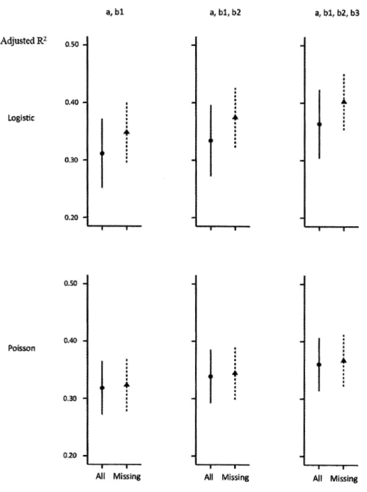
1.3.5 Missing predictors scenario - logistic regression case ... 32
1.4 Results ... 33
1.4.2 Simulation study considering two groups of predictors and assessment of GLM Poisson and logistic measures of explained variation through variation
partitioning ... 35
1.5 Discussion ... 40
CHAPTER II ASSESSING THE ROLE OF COMMUNITY COMPOSITION AND ABIOTIC FACTORS IN PREDICTING FISH SPECIES DISTRIBUTIONS ... 43
2.1 Summary ... 43
2.2 Introduction ... 44
2.3 Methods ... 47
2.3.1 Fish-environment data source ... 47
2.3.2 Target fish species ... 52
2.3.3 Species distribution modelling approaches ... 56
2.4 Results ... 59
2.4.1 Fish species distribution models' quality-of-fit assessment via deviance estimation ... 59
2.4.2 Assessment of predictive accuracy ... 62
2.4.3 Patterns of co-occurrence in freshwater fish species, abiotic parameters and community composition ... 70
2.4.4 Models' agreement and variable importance assessment ... 74
2.5 Discussion ... 92
CHAPTERIII EFFECTS OF ABIOTIC FACTORS ON THE BIOMASS OF SIX FISH SPECIES IN ONTARIO LAKES ... 107
3.1 Summary ... 107
3.2 Introduction ... 108
3.3.1 Fish-environment data source ... 118
3 .3 .2 Lake Selection ... 118
3.3.3 Fish community sampling ... 119
3.3.3.1 BPUE ... 120
3.3.4 Environmental predictors and angling score ... 121
3.3.5 Statistical analyses ... 125
3 .4 Results ... 126
3.4.1 Environmental determinants of species biomass ... 132
3.4.2 Comparison of biomass and occurrence models ... 135
3.4.3 Seeking model parsimony: a comparison between models using the set 3 and 4 of predictors ... 138
3 .4.4 Responses of BPUE from all six freshwater fish species according to the different environmental determinants ... 142
3.4.4.1 Climate ... 146 3.4.4.2 Lake morphometry ... 147 3.4.4.3 Water chemistry ... 148 3.4.4.4 Angling score 149 3 .5 Discussion ... 150 CONCLUSION ... 165 APPENDIX A ... 171 APPENDIX B ... 173 APPENDIX C ... 177 APPENDIX D ... 179 REFERENCES ... 183
covariate was included to the model in the sample size influence assessment, while samples were based on 1 OO observations in the number of inserted random covariates influence case... 34 1.2 The influence of missing covariates on R2 estimation. Values are
expressed as mean ± standard deviation. "a" stands for intercept while "bl", "b2" and "b3" stand for the first, second and third slopes, respectively... .. 36 1.3 The influence of sample size on fraction estimation accuracy,
expressed as mean absolute error (Y axis), in R2 variation
partitioning according to varying levels of correlation between X
and W... 38
1.4 The influence of insertion of random N (0, 1) covariates on fraction estimation accuracy, expressed as mean absolute error, in R2 variation partitioning. Samples were based on 1 OO observations. The degree of correlation between X and W is equal to 0.4... ... 39 2.1 Distribution of the lakes surveyed across Ontario and compiled in
the Aquatic Habitat Inventory... .. . .... .. ... .. ... ... .. .. . .. . ... .. .. 49 2.2 Latitudinal gradient in climate, represented by mean annual air
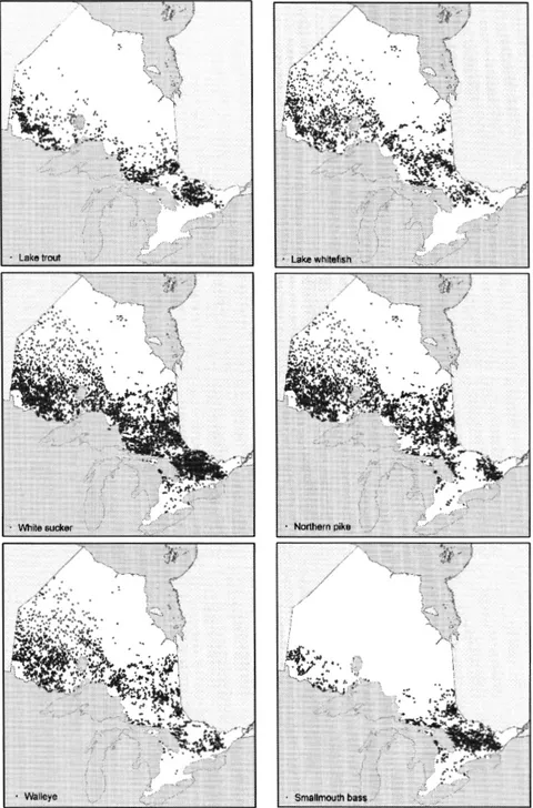
temperature measurements across Ontario... 50 2.3 Distribution of the six freshwater fish species across Ontario,
compiled in the Aquatic Habitat Inventory... . . . 54 2.4 Models' adjusted deviance for all six freshwater fish species target
of this study, according to the three model specifications: (A) models including only abiotic variables, (B) models using only biotic information, and (A+B) models incorporating both abiotic and biotic variables. GLM: generalized linear model based on Poisson distribution; GAM: generalized additive model; MARS: multivariate adaptive regression splines; RF: random forests; BRT: boosted regression trees. . . 61 2.5 Model evaluation assessment through AUC and TSS across all
species' models. Computations were done for (A) models including only abiotic variables, (B) models using only biotic information, and (A+B) models incorporating both abiotic and biotic variables. Models' labels provided in Figure 2.4... 63 2.6 Model evaluation assessment through AUC and TSS for lake trout 64
models. Computations were done for (A) models including only abiotic variables, (B) models using only biotic information, and (A+B) models incorporating both abiotic and biotic variables. Models' labels provided in Figure 2.4 ... . 2.7 Model evaluation assessment through AUC and TSS for lake whitefish models. Computations were done for (A) models including only abiotic variables, (B) models using only biotic information, and (A+B) models incorporating both abiotic and biotic variables. Models' labels provided in Figure
2.4...
65 2.8 Model evaluation assessment through AUC and TSS for walleyemodels. Computations were done for (A) models including only abiotic variables, (B) models using only biotic information, and (A+B) models incorporating both abiotic and biotic variables. Models' labels provided in Figure 2.4. . . 66 2.9 Model evaluation assessment through AUC and TSS for northem
pike models. Computations were done for (A) models including only abiotic variables, (B) models using only biotic information, and (A+B) models incorporating both abiotic and biotic variables. Models' labels provided in Figure 2.4... 67 2.10 Model evaluation assessment through AUC and TSS for white
sucker models. Computations were done for (A) models including only abiotic variables, (B) models using only biotic information, and (A+B) models incorporating both abiotic and biotic variables. Models' labels provided in Figure 2.4. . . 68 2.11 Model evaluation assessment through AUC and TSS for
smallmouth bass models. Computations were done for (A) models including only abiotic variables, (B) models using only biotic information, and (A+B) models incorporating both abiotic and biotic variables. Models' labels provided in Figure 2.4... ... 69 2.12 Model agreement assessment for lake trout, obtained for (A)
models including only abiotic variables, (B) models including only biotic information, and (A+B) models incorporating both abiotic and biotic parameters. GLM: generalized linear model based on Poisson distribution; GAM: generalized additive model; MARS: multivariate adaptive regression splines; RF: random forests; BRT: boosted regression trees; MAX: MAXENT... 75 2.13 Model agreement assessment for lake whitefish, obtained for (A)
models including only abiotic variables, (B) models including only biotic information, and (A+B) models incorporating both abiotic and biotic parameters. GLM: generalized linear model based on Poisson distribution; GAM: generalized additive model; MARS: multivariate adaptive regression splines; RF: random forests; BRT: 76
boosted regression trees; MAX: MAXENT ... . 2.14 Madel agreement assessment for walleye, obtained for (A) models
including only abiotic variables, (B) models including only biotic information, and (A+B) models incorporating both abiotic and biotic parameters. GLM: generalized linear model based on Poisson distribution; GAM: generalized additive model; MARS: multivariate adaptive regression splines; RF: random forests; BRT: boosted regression trees; MAX: MAXENT... 77 2.15 Madel agreement assessment for northern pike, obtained for (A)
models including only abiotic variables, (B) models including only biotic information, and (A+B) models incorporating both abiotic and biotic parameters. GLM: generalized linear model based on Poisson distribution; GAM: generalized additive model; MARS: multivariate adaptive regression splines; RF: random forests; BRT: boosted regression trees; MAX: MAXENT... 78 2.16 Madel agreement assessment for white sucker, obtained for (A)
models including only abiotic variables, (B) models including only biotic information, and (A+B) models incorporating both abiotic and biotic parameters. GLM: generalized linear model based on Poisson distribution; GAM: generalized additive model; MARS: multivariate adaptive regression splines; RF: random forests; BRT: boosted regression trees; MAX: MAXENT... 79 2.17 Madel agreement assessment for smallmouth bass, obtained for (A)
models including only abiotic variables, (B) models including only biotic information, and (A+B) models incorporating both abiotic and biotic parameters. GLM: generalized linear model based on Poisson distribution; GAM: generalized additive model; MARS: multivariate adaptive regression splines; RF: random forests; BRT: boosted regression trees; MAX: MAXENT... 80 2.18 Ranked variable importance obtained for (A) models including only
abiotic variables. Variable importance was computed as an average across all species. GLM: generalized linear model based on Poisson distribution; GAM: generalized additive model; MARS: multivariate adaptive regression splines; RF: random forests; BRT: boosted regression trees; MAX: MAXENT... 82 2.19 Ranked variable importance obtained for (B) models including only
biotic variables. Variable importance was computed as an average across all species. Models' labels provided in Figure 2.18. P _LaTro: presence of lake trout; P _La Whi: presence of lake whitefish; P _ Walle: presence of walleye; P _NoPik: presence of northern pike; P _ WhSuc: presence of white sucker; P _SmBas: presence of smallmouth bass. . . 83 2.20 Ranked variable importance for lake trout, obtained for (A) models 86
including only abiotic variables, (B) models including only biotic information, and (A+B) models incorporating both abiotic and biotic parameters. Variable importancewas computed as an average across all models ... 2.21 Ranked variable importance for lake whitefish, obtained for (A) models including only abiotic variables, (B) models including only biotic information, and (A+B) models incorporating both abiotic and biotic parameters. Variable importance was computed as an average across all models. ... 87 2.22 Ranked variable importance for walleye, obtained for (A) models
including only abiotic variables, (B) models including only biotic information, and (A+B) models incorporating both abiotic and biotic parameters. Variable importancewas computed as an average across all models. ... 88 2.23 Ranked variable importance for northern pike, obtained for (A)
models including only abiotic variables, (B) models including only biotic information, and (A+B) models incorporating both abiotic and biotic parameters. Variable importance was computed as an average across all models. ... 89 2.24 Ranked variable importance for white sucker, obtained for (A)
models including only abiotic variables, (B) models including only biotic information, and (A+B) models incorporating both abiotic and biotic parameters. Variable importance was computed as an average across all models. ... 90 2.25 Ranked variable importance for smallmouth bass, obtained for (A)
models including only abiotic variables, (B) models including only biotic information, and (A+B) models incorporating both abiotic and biotic parameters. Variable importance was computed as an average across all models. ... 91 3.1 Schema of four principal environmental determinants as configured
and entrained by the morphology of an ecosystem, in this case, habitat. The four determinants are comprised of two energetic factors (light and heat) and two material factors (nutrients and oxygen). Light and nutrients are controlling in the sense that they influencebehavior and metabolism, but are rarelylethalat any level found in nature. Heat and oxygen are controlling in their intermediate ranges, but may be limiting at the extremities, and therefore are often lethal. Ex tract from R yder and Kerr
(1989)...·...·...;..~ 112
3.2 Distribution of the sampled lakes across Ontario during the first cycle of theBsM program ... 119 3.3 Explained deviance from boosted regression trees analyses to
3.4 Mean squared error (MSE)/ Mean BPUE estimated from boosted
3.5
3.63.7
3.8
3.9a 3.9b 3.9c3.10
3.113.12
3.133.14
regression trees analyses to predict BPUE of six freshwater fish species ... . Variable relative importance plots generated from boosted regression trees analyses to predict BPUE of six freshwater fish species, using the full set of predictors ... . Variable relative importance plots generated from boosted regression trees analyses to predict BPUE of six freshwater fish species, using the set 2 of predictors ... . Variable relative importance plots generated from boosted regression trees analyses to predict BPUE of six freshwater fish species; using the set 3 of predictors ... . Variable relative importance plots generated from boosted regression trees analyses to predict BPUE of six freshwater fish species, using the set 4 of predictors ... . Partial dependence plots generated from boosted regression tree analyses, showing the responses of BPUE to climate variables for cold water, cool water and warm water freshwater fish species ... . Partial dependence plots generated from boosted regression tree analyses, showing the responses of BPUE to lake morphometry variables for cold water, cool water and warm water freshwater fish species ... . Partial dependence plots generated from boosted regression tree analyses, showing the responses of BPUE to water chemistry variables and angling score for cold water, cool water and warm water freshwater fish species ... . Perspective plot generated from the boosted regression tree model developed for walleye, showing the responses of BPUE to the interaction between MAT and DD5 ... . Perspective plot generated from the boosted regression tree model developed for northern pike, showing the responses of BPUE to the interaction between MAT and DD5 ... . Perspective plot generated from the boosted regression tree model developed for walleye, showing the responses of BPUE to the interaction between DOC and TP ... . Perspective plot generated from the boosted regression tree model developed for northern pike, showing the responses of BPUE to the interaction between DOC and TP ... . Perspective plot generated from the boosted regression tree model developed for northern pike, showing the responses of BPUE to the
131 134 136
140
141
143
144
145
154
155
157
158
158
3.15
interaction between DOC and TP ... . Perspective plot generated from the boosted regression tree model developed for lake trout, showing the responses of BPUE to the interaction between pH and mean depth ... .
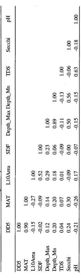
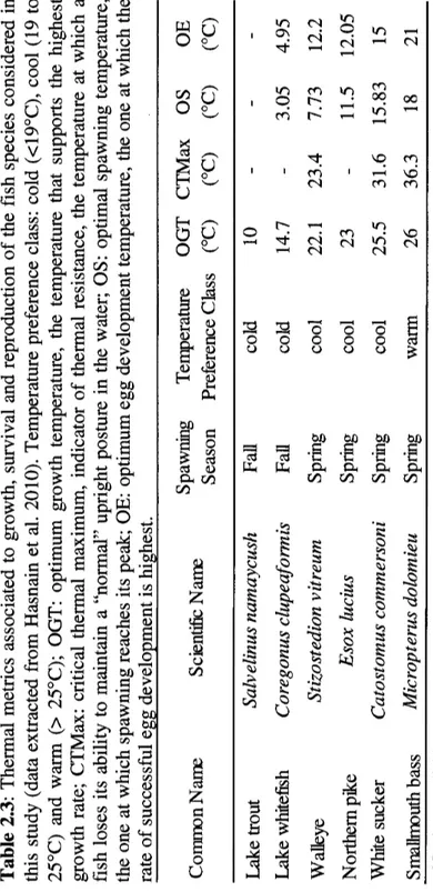
2.2 Pearson correlations among abiotic parameters... .. 51 2.3 Thermal metrics associated to growth, survival and reproduction of
the fish species considered in this study (data extracted from Hasnain et al. 2010). Temperature preference class: cold (<19°C), cool (19 to 25°C) and warm (> 25°C); OGT: optimum growth temperature, the temperature that supports the highest growth rate; CTMax: critical thermal maximum, indicator of thermal resistance, the temperature at which a fish loses its ability to maintain a "normal" upright posture in the water; OS: optimal spawning temperature, the one at which spawning reaches its peak; OE: optimum egg development temperature, the one at which the rate of successful egg development is highest... . . . .. 55 2.4 Relationships' directionality among the six freshwater fish species
and the variables used as predictors in (A) models.
"+"
represents a positive influence of a given variable and"-" represents a negative influence... 72 2.5 Relationships' directionality among the six freshwater fish speciesand the variables used as predictors in (B) models.
"+"
represents a positive influence of a given variable and "-" represents a negative influence. P _LaTro: presence of lake trout; P _La Whi: presence of lake whitefish; P _ Walle: presence of walleye; P _NoPik: presence of northern pike; P _ WhSuc: presence of white sucker; P _SmBas:presence of smallmouth bass. . . 72 2.6 Relationships' directionality among the six freshwater fish species
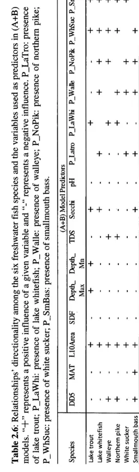
and the variables used as predictors in (A+B) models.
"+"
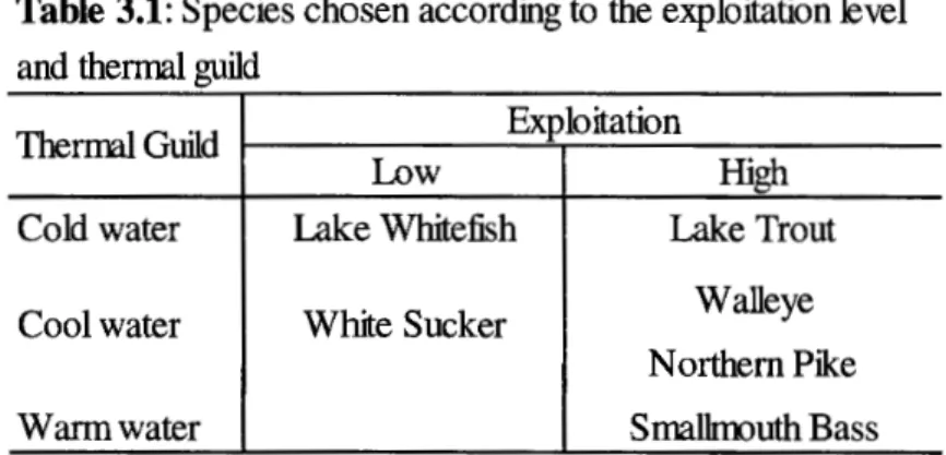
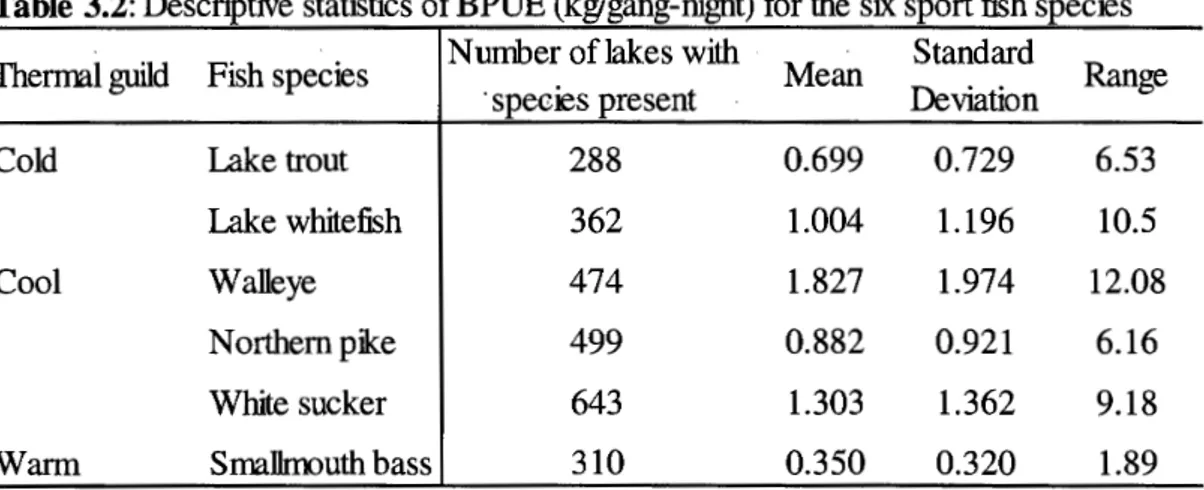
represents a positive influence of a given variable and "-" represents a negative influence. P _LaTro: presence of lake trout; P _La Whi: presence of lake whitefish; P _ W alle: presence of walleye; P _NoPik: presence of northern pike; P _ WhSuc: presence of white sucker; P _SmBas: presence of smallmouth bass... 73 3 .1 Species chosen according to the exploitation level and thermalguild. .. . .. . .. .. ... . .. . ... .. . . ... . . ... .... .. ... . .. ... .. . .. . .. . ... ... . .. ... .. . .... 117 3.2 Descriptive statistics of BPUE (kg/gang-night) for the six
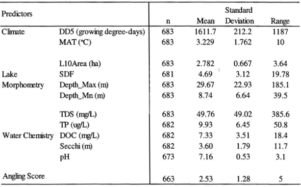
freshwater fish species. . . 121 3.3 Descriptive statistics of all environmental predictors and fishing
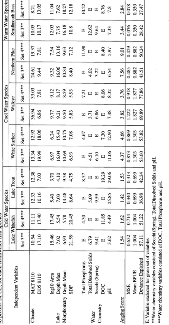
3.4 3.5a
3.5b
2= 1.1-5 hr.ha-1.yr-1; 3= 5.1-10 hr.ha-1.yr-1; 4= 10.1-20 hr.ha-1.yr-1;
5= 20.1-40 hr.ha-1.yr-1 and 6= 40.1
+
hr.ha-1.yr-Pearson correlations among BPUE predictors ... . Variable relative importance, mean squared error and adjusted deviance obtained from boosted regression trees developed to predict BPUE, for each freshwater fish species ... .. Variable relative importance, mean squared error and adjusted deviance obtained from boosted regression trees developed to predict BPUE, for each freshwater fish species ... ..
124
128
modélisation écologique et la quantification des relations espèces-environnement est un élément clé pour la conservation et la gestion des écosystèmes et des populations. L'objectif général de cette thèse est d'améliorer les méthodes quantitatives en : (i) construisant une approche pour les donnée multi-espèces basée sur les modèles linéaires généralisés, appelée "Analyse de Redondance Généralisée" (gRDA); (ii) améliorant la modélisation de la distribution des poissons (présence/absence) en considérant les interactions biotiques entre espèces, et en utilisant les connaissances générées par ces modèles pour (iii) modéliser la biomasse des poissons, déterminer les principaux facteurs environnementaux qui influencent la biomasse des différentes espèces, ainsi qu'évaluer l'impact de la pression exercée par le pêche. Ces liens peuvent contribuer à renforcer la recherche sur la relation espèces-habitat, les services écosystémiques tout en apportant des informations sur les processus qui sous-tendent ces relations. La recherche sur des méthodes quantitatives interconnectées devrait permettre de mieux comprendre les agents qui structurent la biodiversité et comment ils interagissent pour fournir des services écosystémiques, tout en clarifiant les actions qui devraient être entreprises pour remédier à la perte de ces services liées à l'augmentation de l'impact de l'homme. Dans le Chapitre 1, une méthode multi-espèces appelée "Analyse de Redondance Généralisée" (gRDA) a été développée. Cette méthode est basée sur la distribution logistique et la distribution de Poisson, et elle a été étendue au Partitionnement de Variation. Le but du chapitre est de présenter cette méthode et de déterminer ces performances en utilisant une variété de méthodes de Monte Carlo. Nos résultats montrent que la méthode proposée est robuste et devrait remplacer le Partitionnement de Variation standard basé sur l' Analyse de Redondance ordinaire. Le chapitre II présente une comparaison de la performance et de la capacité prédictive de plusieurs méthodes de modélisation de la distribution des espèces, tout en identifiant les prédicteurs les plus importants pour expliquer la présence ou l'absence des espèces considérées. Ces modèles diffèrent par l'utilisation de données empiriques et ont été développés pour six espèces de poisson de l'eau douce dans les lacs d'Ontario. La modélisation dans le chapitre 2 prend en compte trois classes de modèles : (i) les modèles qui n'utilisent que l'information sur les conditions environnementales comme prédicteurs: (ii) ceux qui utilisent uniquement l'information sur les communautés de poissons pour prédire la présence d'une espèce particulière (c.à.d. variables abiotiques) et (iii) une combinaison de (i) et (ii) (c.à.d. variables abiotiques et biotiques). Finalement, en utilisant les mêmes espèces de poissons que pour le Chapitre II, le chapitre III présente des modèles de biomasse développés au moyen d'arbres de régression permettant d'identifier l'importance
relative de différentes variables environnementales ainsi que la pression angulaire. De plus, les similarités et différences entre guildes de poissons ont été mises en évidence par l'influence de chacun des prédicteurs sur la biomasse de chaque espèce. Les résultats des chapitres II et III révèlent l'importance de la morphométrie des lacs et du climat pour l'estimation de la présence/absence et de la biomasse, et, dans le chapitre II particulièrement, il a été observé que les modèles de présence/absence ont de meilleures performances lorsqu'ils tiennent en compte de l'information biotique ainsi que des prédicteurs abiotiques. De plus, les résultats indiquent que la performance des modèles pourrait être largement affectée par la manière dont ces modèles sont développés et évalués. Choisir une méthode de modélisation appropriée, les variables explicatives, les méthodes de validation et les mesures de performances sont des étapes importantes pour obtenir des inférences ou prédictions plus fiables plutôt que des résultats spécifiques aux données ou des artéfacts statistiques. De ce fait, la présente thèse fournit une enquête complète sur l'amélioration des méthodes de modélisation populaires, tout en montrant leurs utilités pour évaluer l'importance des facteurs influençant la distribution et la biomasse des poissons qui ont une importance économique en Ontario, ce qui peut être utile du point de vue de la gestion des ressources naturelles.
Mots-clés: modélisation écologique; Analyse de Redondance; Partitionnement de Variation; modélisation de la distribution des espèces; modèles de biomasse; Poisson d'Eau Douce.
quantification of species-environment relationships is critical for conservation planning and ecosystem/population management. The general objective of this thesis is to improve quantitative methods to: (i) build a framework for multispecies data based on generalized linear models, called "Generalized Redundancy Analysis" (gRDA); (ii) access improvement in species distribution modelling approaches developed for fish presence-absence by inserting biotic information related to the fish species, and knowledge about these models are linked to the (iii) development of fish biomass models while unravelling the principal environmental determinants that influence the biomass of different species, when also evaluating the impact of fishing pressure. These links can contribute to major scientific underpinnings related to the research of species-habitat relationships, while consisting of ecosystem services when promoting information about the processes underlying these relationships. The investigation of interconnected quantitative frameworks to link environmental, spatial and biotic interactions should bring to light a greater understanding of the key agents structuring biodiversity and how they interact to provide the delivery of aquatic ecosystem services, while clarifying about the actions that should be taken to mitigate the loss of these services in face of increasing human impacts. In Chapter 1, a multispecies framework called "Generalized Redundancy Analysis" (gRDA) was developed, based on logistic and Poisson distributions via GLMs, and extend this framework to variation partitioning. The goal was to present the framework as well as assess its performance using Monte Carlo approaches under a variety of scenarios. Our results showed that the proposed framework is very robust and should essentially replace the current standard variation partitioning based on ordinary Redundancy Analysis. Chapter II presents a comparison among a number of SDM approaches in terms of their predictive performance and explanatory power, while identifying the predictors that are most influent in explaining presence-absence of the species considered. These models were contrasted by using empirical data and developed for six species of freshwater fishes in north-temperate lakes of Ontario. The modelling routine for Chapter 2 was done taking into account three classes of models (i) incorporating only information about the environmental features as predictors; (ii) using solely the information about the fish community to predict the occurrence of a particular species (i.e. using biotic parameters) and (iii) represents a combination of (i) and (ii) (i.e. using abiotic
+
biotic parameters); Finally, using the same fish species from Chapter II, Chapter III presents biomass models developed via boosted regression trees, allowing to identify the relative importance of the different principal environmental determinants used as regressors, together with angling pressure. Inaddition, sirnilarities and dissirnilarities within and among fish thermal guilds were showcased regarding the biomass response of each species to every predictor used in the modelling process. Results from Chapter II and III point out the importance of lake morphometry and climate to the estimation of presence-absence and biomass, and in Chapter II particularly it was observed model improvements when biotic information was used together with abiotic predictors for presence-absence models. In addition results indicated that model performance could be largely affected by how models were developed and evaluated. How to choose appropriate modelling approaches, predictor variables, model validation methods, and performance metrics are important steps if we want to get more reliable inferences or predictions rather than data-specifics results or statistical artifacts. Thus, this thesis provides a comprehensive investigation on aspects consisting of improvements of popular modelling approaches, while showing their usefulness in assessing important information related to factors most influent in the distribution and biomass of econornically important fish species in Ontario, which can be useful from the natural resources management point of view.
Keywords: ecological modelling, Redundancy Analysis, Variation Partitioning, species distribution models, biomass models, freshwater fish
part refers to a discussion about the role and increasing importance of species distribution modelling in Ecology, showing the different steps involved in the calibration (building) process, the importance of each of these steps, followed by the importance of proper estimation, addressing the most common limitations faced when building static and probabilistic models. The second part outlines ecosystem services and the importance of different services provided by fish populations. 1 will address the importance of the development and assessment of models and quantitative tools to better predict and understand the ecosystem services provided by fish, focusing on how this information can improve monitoring and management programs for fish populations.
0.1 Species modelling
The analysis of species-habitat relationships has always been a central goal in ecology. lt has become a central framework to explore, understand and tackle specific questions about the intricacies and mechanisms underlying species distributional patterns in space and time. The savoir-faire generated by ecological modelling and its quantification of species-environment. relationships is critical for conservation planning and ecosystem/population management. The statistical frameworks applied in ecological modelling are generally based on estimating parameters about the importance of environmental features (e.g., local habitat, regional climate, habitat connectivity) influencing the distribution of species and their communities (Guisan
and Zimmermann 2000). This knowledge is of utmost importance to estimate habitat suitability for endangered species, discover new populations or previously unknown species, forecast effects of habitat change due to human interference, establish potential locations for species reintroduction, predict how community structure may be affected by the invasion of exotic species, predict the eff ect of ecological disturbances, climate change or how environmental conditions affect different communities across different spatial/temporal scales. Habitat models relating habitat characteristics, and species distributions and community structure allows one to derive/predict the habitat potential distribution within the modelled area, which is equivalent to modelling its potential habitat (Schuster 1994) and niche (Elith and Leathwick 2009). A plethora of statistical approaches for species modelling are available (e.g. Harvey 1978; Somers and Harvey 1984; Legendre and Fortin 1989; Jackson and Harvey 1993; Jenkins and Buikema 1998; Guisan and Zimmermann 2000; Peres-Neto et al. 2006; Sharma and Jackson 2007; Elith et al. 2008 and many others) and they differ in their ability to model environmental relationships. As such, an evaluation of different statistical techniques can provide insights into which approaches are most appropriate for the biological question being asked at both the species and community levels (Guisan and Zimmermann 2000; Elith et al. 2006; Sharma and Jackson 2008; Sharma et al. 2012). It is important to keep in mind that habitat models are expected to address at least two questions: ( 1) how well the distribution of a set of species is explained given a set of covariates? (2) Which covariates are unimportant in the sense of contribution to the explanation of patterns already accounted for by other variables present in the model (i.e., marginal and independent contribution).
The development of environmental niche models involves some steps that are central while generating a consistent tool that works with similar levels of accuracy across large landscapes, particularly in those in which the nature of the covariation among
predictors and their contribution to species distributions change spatially (e.g., non-stationarity; Wenger and Olden 2012). The first step is the conceptual model formulation, or underlying conceptual framework. In this step, one usually faces the task of deciding which model properties are desirable to achieve. Levins (1966) points out three main model properties, generality, reality and precision, stating that only any two out of three can be improved simultaneously. In this sense, three classes of models can be designed: (i) accurate prediction within a limited or simplified reality. In this category, analytical (Sharpe 1990) models are suitable and they incorporate precision and generality; (ii) predictions attained on real cause-effect interactions are named mechanistic (Prentice, 1986), designed to be realistic and general, with a focus on theoretical correctness of the predicted response over predicted precision; (iii) Empirical models (Decoursey 1992) are based on precision and reality, condensing empirical facts instead of considering realistic "cause and effect" between response and explanatory variables. Central aspects to consider when conceptualizing a predictive habitat distribution model are the inclusion of direct
versus indirect (e.g., proxy) predictors, the choice of modelling the fundamental
versus the realized niche (Kearney and Porter 2009), to assume equilibrium between
environment and observed species patterns versus non-equilibrium (Hof et al. 2012) and individual species modelling versus community approach (Ferrier and Guisan 2006). Note that the choice of an appropriate spatial scale (Wiens 1989), selection of a set of conceptually meaningful explanatory variables and designing an efficient sampling strategy are equally important when formulating a given model and its objectives.
The second step in the development of empirical ecological niche models is the statistical model formulation. In other words, the choice of the statistical technique to be applied in order to model the relationship between the response and explanatory variables. The type of response variable (quantitative, semi-quantitative, qualitative)
and its probability distribution has also a great influence on the selection of an appropriate technique. Sorne of the most popular species distribution modelling approaches comprises:
(i) Linear regression methods, which can be extended to mode! complex data types (e.g. fixed versus random covariates) and allow the inclusion of additive combinations of predictors and/or terms representing interactions between predictors;
(ii) GLMs, extensively used by ecologists for its ability to deal with data possessing different error structures, particularly presence/absence modelled via logistic regression. They consist of mathematical extensions of linear models that do not force data into unnatural scales, also allowing for nonlinearity and nonconstant variance structures in data;
(iii) Generalised Additive Models (GAMs, Hastie and Tibshirani 1990), which consist of a powerful extension of GLMs, gaining increasing popularity due to the ability of defining non-parametric smoothers to describe nonlinear responses, contributing with useful flexibility for fitting ecologically realistic associations;
(iv) Multivariate Adaptive Regression Splines (MARS, Friedman 1991) combines the strengths of regression trees with piecewise linear basis fonctions, which allows the modelling of complex relationships while possessing exceptional analytical speed;
(v) Ordination techniques, more specifically direct gradient analysis, providing axes that are constrained to be a fonction of environmental factors, i.e., sample scores are constrained to be linear combinations of explanatory variables. Canonical Correspondence Analysis (CCA) and Redundancy Analysis (RDA) are noteworthy approaches;
(vi) Classification tree analysis (CTA, Breiman et al. 1984, also referred to as classification and regression trees - CART) are machine-learning methods
for constructing prediction models from data. The models are obtained by recursively partitioning the data space and fitting a simple prediction mode! within each partition. Trees explain variation of a single or multiple response variable by repeatedly splitting the data into more homogeneous groups, being each characterized by a typical value of the response variable, the number of observations in the group, and the values of the explanatory variables that specify it;
(vii) Artificial neural networks (ANN, Olden et al. 2008), whose information processing system is composed of a large number of highly interconnected elements called "neurons", working together to solve specific problems. They are popular in Ecology because they are considered to be universal approximations of any continuous fonction, being quite popular when modelling nonlinear relationships. Their full classification procedure is a complex non-parametric process;
(viii) Random forests (RF, Prasad et al. 2006), which creates multiple boot-strapped regression trees without pruning and averages the outputs, with each tree being grown with a subset of predictors entered in the mode! in a random order to avoid bias due to the inter dependencies among predictors. Typically a large number of trees is grown (500 to 2000), creating a limited generalization error, and thus reducing overfitting; (ix) Boosted regression tree (BRT, Elith et al. 2008) improves the performance
of a single mode! by fitting many models and combining them for prediction, using two algorithms: regression trees (from the classification and decision tree group of models) and boosting builds, which combines a collection of models. For regression problems, boosting is a form of "functional . gradient desœnt", a numerical optimization technique for minimizing the loss fonction by adding, at each step, a new tree that best reduces ( steps down the gradient of) the loss fonction. The first tree is the one that maximally reduces the loss fonction, followed by a tree that is
fitted to the residuals of this first tree, which can contain quite different variables and split points compared with the first. The model is then updated to contain two trees (two terms), and the residuals from this two-term model are calculated, and so on. The final BRT model is a linear combination of many trees that can be thought of as a regression model where each term is a tree. BR Ts have been showing interesting results, possessing the ability to account for uncertainty in model structure;
(x) Maximum entropy (MaxEnt, Phillips et al. 2006) estimates a target probability distribution by finding the probability distribution of the maximum entropy (in other words, that is most spread out, leading to uniform), subject to a set of constraints that represent incomplete information about the target distribution. lt bas gained popularity among studies that entail presence-only data (e.g., museum data), but can also be applied to presence/absence data by using a conditional model.
After selecting a given statistical approach, the model is calibrated on real data. Rykiel (1996) defines calibration as "the estimation and adjustment of model parameters and constants to improve the agreement between model output and a data set". However, the selection of proper explanatory variables is a vital component of this process. In an ideal modelling world, a model should be parsimonious, i.e.,
should accomplish its desired level of explanation or prediction with as few predictor variables as possible, and this can be a difficult task since nature is not completely parsimonious. Due to the recognition of (living) nature as an extremely complex phenomenon, driven by several factors interacting at the same time, and in different orders of magnitude. One particular challenge to keep in mind is that parsimony is often obtained by the trade-offs between predictive power and complexity, and not necessarily taking into account how well we understand variable contribution to the model. For instance, two models may have similar predictive power and amount of
predictors, but one is much easier to explain based on current knowledge of how a predictor is likely to affect the response. The choice of predictors can be done arbitrarily (which is not recommended for its inconsistency), automatically (via stepwise procedures available in linear regression methods and GLMs), following physiological and other ecological or mechanistic principles or by shrinkage rules (Harrell et al. 1996). After variable selection, model parameters are estimated and its fit is characterized, most of the time, by a measure of the variance reduction (or deviance reduction in maximum likelihood techniques). The model optimization through deviance reduction is performed through an estimated
D2 (
equivalent to R2 in least-squares models), being defined as:D2 = Null deviance-Residual deviance Null deviance
where the null deviance is the deviance of the model with the intercept only, and the residual deviance is the one that remains unexplained by the model after the insertion of all selected predictors. The ideal model has no residual deviance and its D2 equals
one. Weisberg (1980) argues that the deviance formulation is not representative of the real fit, and proposes an adjusted version based on the number of observations n and the number of predictors p, which bas been largely adopted:
n-1
adjusted D2 = 1 - - -
x
(1 - D2 )n-p
The value of the adjusted D2 increases with an increasing n or a decreasing p in the model, and it allows for comparisons among nested models that include different combinations of explanatory variables. In tree-based approaches, no fit needs to be characterized since the model will attempt to predict the data exactly. Diagnostic tests for significance of estimated model coefficients can be performed based on the related variance or deviance distribution in least-squares and GLM estimation.
After model calibration, the next step consists of evaluating the model, also called
model validation, which is the measurement of adequacy between model predictions
and field observations, depending mostly on the specific purpose of the research and the domain in which the model is supposed to be applicable (Fielding and Bell 1997). Two main approaches are worth mentioning: (i) using a single data set to both calibrate and validate the model via cross-validation (V an Houwelingen and Le Cessie 1990), leave-one-out Jackknife (Efron and Tibshirani 1993) or bootstrap (Efron and Tibshirani 1993); (ii) having two independent data sets, using one for calibration and the other for validation, this approach being optimal and attractive. The first approach is usually selected when the data set is too small to be split into separate data sets but often used for large data sets as well. Regardless of the approach, two types of measure can be used to quantify the fit between predicted and observed values of the validation data set: (i) using the same goodness-of-fit methods used to calibrate the model or (ii) using any discrete measure of association between predicted and observed values (Guisan and Harrell 2000). In the case of presence-absence data (binary), probabilities are truncated at an adjusted optimal threshold (below threshold being predicted absent and above as present) that provides the best agreement between predicted and observed values. A confusion matrix (Guisan et al. 1998) expressing the number of true positives (predicted and observed present), true negatives (predicted and observed absent), false positives (predicted present but observed absent) and false negatives (predicted absent but observed present) is then analysed through the proportion of area correctly classified, the percentage of commission and omission errors, or using Cohen's K (Cohen 1960), among other
metrics. Another option for binary datais the use of a threshold-independent measure like the receiver operating characteristic (ROC) plot methodology (Fielding and Bell 1997). For quantitative data, the evaluation of predictions can be done simply by using Pearson's product-moment correlation coefficient if the variable is normally
distributed, or a non-parametric rank correlation coefficient like Kendall's 't or Spearman's
p.
With the increasing number of studies on predictive habitat distribution modelling, some key topics related to their limitations appear frequently and they comprise potential areas of investigation:
• Multiple scales: all species fonction at specific spatial and related temporal scales. However, their joint localized activities mediate processes that are important at the landscape scale (Anderson 1993). A hierarchy of scale-dependent abiotic factors, biotic interactions, population processes, disturbances and legacies govern their distribution (Ettema and W ardle 2002). Given this fact, species distribution modelling should either focus on appropriate scales that are relevant to the research question, the system, data availability or simultaneously consider multiples scales (Beever et al. 2006). Conceptually, there is no single natural scale at which ecological patterns should be studied (Levin 1992).
• Biotic interactions: most SDMs are calibrated under the assumption that biotic interactions do not influence species range patterns (Huntley et al. 1995) or only affect patterns at small spatial scales (Pearson and Dawson 2003). Recent developments aim at considering abiotic interactions (e.g., Boulangeat et al. 2012), though these approaches remain in their early stages. In models for understanding or interpolation-style prediction, the consequences may not be too severe, except where the presence of a host species is critical and not predicted by the available covariates. Studies were published showing how the incorporation of biotic interactions into SDMs better models species distributions and responses to environmental change. The information about these interactions is included, for example,
in the form of occurrence (Heikkinen et al. 2007), counts or frequencies (Leathwick and Austin 2001) or as a competition coefficient (Strubbe et al. 2010). The importance of biotic interactions may vary depending on the spatial scale and position along environmental gradients. In models built for extrapolation, like in the case of the effects of climate change on species distributions, the effects of competitors, mutualists and conspecific attractions might have far-reaching effects (Elith and Leathwick 2009). • Uncertainty: it results both from data deficiencies (like missing covariates,
small samples, biased species occurrences, lack of data about absence or inadequate sampling strategy) and from errors in model specification (Barry and Elith 2006). Few studies have addressed uncertainty in SDMs and its effects in model calibration, predictions and associated decision making. In management applications, it is important to investigate the impact of uncertainty and how to reduce it, characterizing and exploring its effects in decision making. Heikkinen et al. (2006) provide some useful information in various aspects of SDMs that contribute to uncertainty. • The use of presence-absence data versus abundance: the relative use of
presence-only and presence-absence data has been widely discussed (Elith et al. 2006), abundance data are available for many taxa in some regions, and it can provide additional information that might be better related to conservation status (Johnston et al. 2013), extinction risk (O'Grady et al. 2004) and community structure and function (Davey et al. 2012). Moreover, SDMs derived from abundance data may reflect the importance of key demographic and environmental factors such as carrying capacity (Pearce and Ferrier 2001 ). Howard et al. (2014) points out the importance of abundance data in predictive modelling, deriving a more accurate assessment of habitat suitability in contrast to presence-absence data. However, the choice of using presence-absence over abundance cornes, in most cases, from the focus on methodological development to enhance
model performance (Guisan and Thuiller 2005, Elith et al. 2006) or pure lack of abundance data available, the latter being the most restrictive. Comparisons between models based on abundance versus presence-absence data, while addressing other SDM limitations, are the subject of potential future research.
• Spatial autocorrelation (SAC): spatially explicit predictive models are generally built with little or no attention to spatial processes that drive species distributional patterns. SAC occurs when the values of variables sampled at nearby locations are not independent from each other (Tobler 1970). The causes underlying are manifold, but three are worthy of mention: 1) biological processes such as speciation, extinction, dispersal or species interactions; 2) non-linear relationships between environment and species modelled (erroneously) as linear; 3) spatially-structured environmental features impose a spatial structure in the response (Legendre and Fortin 1989, Legendre and Legendre 1998). While spatial autocorrelation can provide information about biotic processes such as population growth, geographic dispersal, differential mortality, social organization or competition dynamics (Griffith and Peres-Neto 2006), if not properly accounted for, it can also cause serious drawbacks for hypotheses testing and prediction as it affects type 1 errors rates and precision in the estimation of model parameters (with the exception of machine-leaming methods such as Random Forests). This is because SAC violates important statistical assumptions such as independently and identically distributed (i.i.d.) errors in both parametric and non-parametric testing (Lennon 2000). There are several approaches to incorporate spatial autocorrelation in statistical models, being these autocovariate regression, spatial eigenvector mapping (SEVM), generalised least squares (GLS), conditional autoregressive models (CAR), simultaneous autoregressive models (SAR), generalised linear mixed models (GLMM) and generalised
estimation equations (GEE), among others. Dormann et al. (2007) addresses a comparison among these methods, reporting their efficiency and flexibility, with some remarks regarding the use of autocovariate regression. That said, different models are likely to be affected differently by spatial autocorrelation (e.g., logistic regression versus regression trees) and systematic comparison of the effects of SAC on model estimation and prediction is largely missing. There is still considerable debate as to whether spatial autocorrelation results in (statistically) biased coefficient estimates, how to best use explicitly spatial methods with incomplete sample data and whether previous studies that used non-spatial methods with spatially autocorrelated data should be considered fraught with error.
0.2 Modelling in the context of aquatic ecosystem services
Ecosystems generate a range of goods and services to society, which in tum directly contribute to our well being and economic wealth (de Groot et al. 2012). Over the past two decades, progress has been made in understanding how ecosystems provide services and how service provisioning translates into economic value (Daily 1997). Ecosystem services the processes whereby ecosystems render benefits to people
-are becoming the principal means for communicating ecological change in terms of human benefits (Daily 1997). Understanding ecosystem services is fondamental to decision-making efforts that influence multiple human activities and components of ecosystems, informing management and planning decisions such as the appropriate scale and location of a number of activities. Wise and sustainable decisions of this nature will require a comprehensive understanding of how changes in human activities and ecosystem states will result in changes in ecosystem services and the associated benefits to people. Valuing the contribution of ecosystems to human
well-being through economic, ecological and social accounting demands robust methods to define and quantify ecosystem services. Y et, it has proven difficult to move from general pronouncements about the' tremendous benefits nature provides to people to credible, quantitative estimates of ecosystem service values. Without quantitative assessments, and some incentives for landowners to provide them, these services tend to be ignored by those making land-use and land-management decisions. Decision making and policy aimed at achieving sustainability goals can be improved with accurate and defendable methods for quantifying ecosystem services (McKenzie et al. 2011).
Currently, there seems to exist a gap between how the regulation of ecosystem services is perceived and how they are managed. At one band, the effects of landscape patterns at different spatial scales on ecological processes and species distributions have long been recognized by scientists and managers as crucial to understanding how such processes fonction (Hobbs 1997) and regulate ecosystem services and their sustainability. On the other band, management strategies for freshwater ecosystem services most often focus on local systems (place-based) such as individual water bodies. Therefore, an integrated multi-scale framework where conservation, management and development of ecosystem services are coordinated is likely to result in the best approach (Abell et al. 2007).
Although an integrated, landscape oriented framework would likely offer improved tools for the effective and sustainable conservation of regional aquatic biodiversity and related services (Lester et al. 2003), knowledge and agreement on how such an approach ·. can best be implemented 1.s lacking. It is of utmost importance to design sampling strategies (field measures, site selection for monitoring) and quantitative frameworks to link ecological indicators of ecosystem health and provide the best
estimates of an ecosystem's capacity to sustainably deliver ecological services. The focus on increasing the understanding of how ecosystem fonction is related to the delivery of aquatic ecosystem services, at several spatial scales, and how to assess the health of these ecosystems is of considerable relevance. Assessing whether ecosystems and their functional ability to deliver services have been impaired (or are at risk or are recovering) requires the possession of robust metrics to determine ecosystem status and trends. Moreover, reliable ecological knowledge regarding aquatic ecosystem services needs to incorporate ways to measure and understand the effect of cumulative impacts on ecosystem health (Duinker and Greig 2006). Finally, by comparing health conditions of different systems and their delivery regarding aquatic ecosystem services, it is possible to establish (1) how multiple natural and anthropogenic stressors interact and affect aquatic ecosystem services; and (2) an understanding of how resilience of biodiversity-ecosystem services is linked to environmental conditions and ecosystem health. This knowledge makes possible the design of landscape-oriented approaches that can provide much more effective information about the status of local and regional aquatic ecosystems and their related services. This is especially important given the growing support for aligning conservation efforts to ecosystem services (Goldman et al. 2008).
Fish populations in aquatic ecosystems benefit human societies in numerous ways, providing: (i) regulating services (e.g., regulation of food web dynamics, recycling of nutrients, regulation of ecosystem resilience, redistribution of bottom substrates, regulation of carbon fluxes from water to atmosphere, maintenance of sediment processes and maintenance of genetic species, ecosystem diversity); (ii) linking services (e.g., linkage within aquatic ecosystems, linkage between aquatic and terrestrial ecosystems, transport of nutrients, carbon, minerals and energy); (iii) cultural services (e.g., production of food, aquaculture production, production of medicine, control of hazardous diseases, control of algae and macrophytes, reduction
of waste, supply of aesthetic values and recreational activities) and (iv) information services (e.g., assessment of ecosystem stress and resilience, revealing evolutionary histories, provision of historical information, scientific and educational information) (Holmlund and Hammer 1999). Certain ecosystem services generated by fish populations are also used as management tools, e.g. enhancing rice production (Tilapia, carp ), mitigating diseases in tropical zones (mosquito contrai) or mitigating algal blooms (pike Esox Lucius). However, increasing fishing pressure, pollution, habitat destruction, introduction of exotic species and other factors continue to exert strong pressure on fish populations around the world (Malakoff 1997). Human-induced direct and indirect degradation of common fisheries resources might cause impacts at the ecosystem level, putting the fondamental and demand-derived ecosystem services generated by fish at risk with consequences for biodiversity and ecosystem resilience (Perrings et al. 1995).
Ecological modelling can provide a way of clarifying which factors and processes drive ecosystem services related to fish, and it is urgently needed. Modification and loss of aquatic habitat is recognized as the primary factor threatening the conservation of fish populations and their communities (Ricciardi and Rasmussen 1999). Species distribution models have a number of important applications to the conservation and management of fish populations and their related ecosystem services, playing an important role in prioritising surveys and monitoring programmes for fish populations because limitations to resources often preclude exhaustive and continuai sampling of sites and that extensive sampling is needed to accurately sample lake fish communities (Jackson and Harvey 1997). Sorne applications include: (i) forecasting or measuring the effects of habitat alteration and changing land-use patterns (Oberdorff et al. 2001); (ii) providing first-order estimates of habitat suitability to establish potential locations for re-introduction (Evans and Oliver 1995); (iii) assess the impacts of the most recent climate change scenarios (Buisson et al. 2008); (iv)
understand the factors that regulate the spread of invasive species and identifying theirpotential distributions (Wang and Jackson 2014); (v) predicting thelikelihoodof local establishment and spread of exotic species that may help set conservation priorities for preserving vulnerable species and populations that might be lostlocally (Peterson and Vieglais 2001). (vi) predicting hotspots of species persistence for the conservation of biodiversity (Williams and Araujo 2000); and (vii) revealing additional populations of threatened species, or altematively revealing unexpected gaps in theirrange. The first step towards a comprehensive assessment of ecosystem goods and services involves translating ecological complexity (abiotic factors and ecological processes) into a more limited number of ecosystem fonctions, which in tum provide ecosystem services (de Groot et al. 2002). The development of broad-scale perspectives to understand the nature, fonction, vulnerability and threats to fisheries-based aquatic ecosystem services are now deemed essential when designing and implementingscientifically-sound management strategies.
0.3 Thesis outline
The goal of this thesis was to conduct an investigation into aspects currently used modelling ~ (more specifically species distribution models), seeking
improvement of these and ultimately provide analytical tools to be applied in ecological assessments related to freshwater fish populations. To this end this thesis is comprised of three chapters, the first one conducted with simulated data and the others applied to freshwater fish data:
Chapter 1: Generalized linearmodels for direct gradient analysis and variation partitioning of species data matrices
Chapter II: Assessing the role of community composition and abiotic factors in predicting fish species distributions
Chapter III: Effects of abiotic factors on the biomass of six fish species in Ontario lakes
Within Chapter 1, 1 developed a framework called gRDA, and evaluated its performance via simulations for modelling multispecies data based on generalized linear models (logistic and Poisson). To date, the most used tool for multi-species modelling is based on linear regression (Gaussian; Legendre and Legendre 1998), which is known to have undesirable properties for presence-absence and abundance data. Moreover, my research within Chapter 1 found that, despite its popularity, logistic regression has extremely bad behaviour in terms of parameter estimation properties under a high number of covariates and when covariates are missing. To remediate this issue, 1 proposed a modified Poisson model that can model presence-absence data and that provides reliable estimates when covariates are missing or the number of covariates is high. Moreover, 1 evaluated the performance of a robust estimate for the coefficient of determination (R2) for GLMs, which allows for the first time an appropriate ·variation partitioning scheme, a widel y used tool in ecology (Peres-Neto et al. 2006), which is currently based on multiple regression.
Chapter II presents a comparison among a number of SDM approaches in terms of their predictive performance and explanatory power in predicting occurrence of six freshwater fish species in north-temperate lakes of Ontario, including the GLM based on Poisson distribution addressed in Chapter 1. These models were contrasted by using empirical data based on the Aquatic Habitat Inventory provided by the Ontario
Ministry of Natural Resources and Forestry. The modelling routine for Chapter 2 was performed taking into account three classes of models: (i) incorporating only environmental parameters; (ii) using solely the information about the fish community to predict the occurrence of a particular species (i.e. using biotic parameters) and (iii) using both environment and the information about the occurrence of other fish species as predictors (i.e. using abiotic + biotic parameters), seeking to identify the influence of biotic information to the predictive ability of these different models. Finally, variable relative importance assessments were also made across models, for each fish species and classes of models, in order to identify which variables were important in predicting presence-absence of a particular species.
Chapter III aimed at the development of biomass models using biomass-per-unit effort (BPUE) information from the same six freshwater fish species mentioned in Chapter 2, using environmental predictors based on principal environmental determinants (light, heat, lake morphometry, nutrients), together with fishing pressure. The species were chosen in order to disentangle the effects of climate and exploitation when evaluating the model results. To this end, four sets of environmental predictors were used: the first one consisted of the full model, which considered all main environmental predictors from the Broad Scale Monitoring program dataset, including angling pressure; the second one kept the same environmental predictors used in Chapter II to develop occurrence models, in order to evaluate the degree of agreement between occurrence (developed in that chapter) and biomass models; the third, a model with secchi depth, total dissolved solids (TDS) and pH encompassing the pool of variables representing water chemistry, in order to compare with the fourth set; the fourth set included total phosphorus (TP) arid dissolved organic carbon (DOC) by replacing secchi depth and TDS from set 3, in order to evaluate which model better optimizes the full model, achieving model parsimony. In addition, variable relative importance was assessed for all models built,
and partial dependence plots were obtained for the optimized model, seeking to evaluate the influence of each environmental feature to the biomass of the six freshwater fish species. These models "brought a better understanding related to the importance of the different environmental determinants in the biomass composition of each species, including existing interactions among main variables influencing biomass.
In summary, Chapter I results provide ecologists with a new GLM-based tool for variation partitioning schemes, consisting of an improvement over the OLS-based ones; Chapter II presents occurrence models considering both abiotic and biotic features, showcasing the importance of adding biotic information when seeking to improve species distribution models developed for six freshwater fish species, and Chapter III investigates the main environmental determinants influencing the biomass of the same six species, while allowing us to assess similarities among the models developed in the last two chapters, and finally making use of one of the modelling approaches that best explained fish occurrence variability in Chapter Il.