Reverse Blending: an economically efficient approach to the challenge of fertilizer mass customization

Int. J. Production Economics 226 (2020) 107603

Available online 27 December 2019

0925-5273/© 2020 Elsevier B.V. All rights reserved.

Reverse Blending: An economically efficient approach to the challenge of

fertilizer mass customization

Latifa Benhamou

_{, Vincent Giard}

_{, Mehdi Khouloud}

_{, Pierres Fenies}

_,

Fr�ed�eric Fontane

a_{EMINES School of Industrial Management, University Mohammed VI Polytechnique, Benguerir, Morocco} b_{Paris II Panth�eon Assas University, Paris, France}

c_{Universit�e Paris-Dauphine, PSL Research University, CNRS, LAMSADE, Paris, France} d_{Fertilizers Unit UM6P-lab OCP-group, 24025, Jorf Lasfar, Morocco}

e_{Mines-Paris Tech, PSL Research University, Paris, France}

A R T I C L E I N F O Keywords:

Mass customization Continuous production Blending

Composite material design Fertilizer

Pooling problem

A B S T R A C T

Reasoned fertilization, which is a major concern for sustainable and efficient agriculture, consists of applying customized fertilizers which requires a very large increase in the number of fertilizer formulae, involving increasing costs due to the multiplication of production batch, of storage areas and of transportation constraints. An alternative solution is given by adopting a Reverse Blending approach, which is a new Blending Problem where inputs are non-pre-existing composite materials that need to be defined in both number and composition, simultaneously with the quantities to be used in the blending process, such as to meet the specifications of a wide variety of outputs, while keeping their number as small as possible. This would replace the production of a large variety of small batches of fertilizers by few large batches of new composite materials whose blending may be performed close to end-users (delayed differentiation), delivering substantial production and logistics cost sav-ings, well in excess of remote blending costs. Reverse Blending presents some analogies with the Pooling Problem which is a two-stage Blending Problem where primary inputs are existing raw materials. An adapted version of this problem may be used to facilitate the design of new composite materials used by Reverse Blending. This paper presents the Reverse Blending approach, whose modelling is based on a quadratic programming formu-lation, and a large case study to demonstrate its feasibility. Reverse Blending, therefore, may be a disruptive approach to successfully reengineer not only the fertilizer supply chain but any other industry operating in blending contexts to meet a great diversity.

1. Introduction

The fertilizer industry faces a major dilemma which is unable to resolve under the current product/process organization. On the one hand, sustainable and efficient agriculture would require hundreds of different customized fertilizers, amounting to a much greater variety than that currently on offer; and on the other hand, such required di-versity cannot be produced at an acceptable cost in the fertilizer plants as they exist today, with continuous production processes geared to batch production. In discrete production, however, mass customization can easily be performed in assembly lines, enabling successive produc-tion of different products. The proposed soluproduc-tion can be considered both

original and disruptive: fertilizer plants need not produce all the fertil-izers required by end users but only a few intermediate products, which are later combined to produce the required fertilizers in small blending units located in the countryside, close to actual fertilizer users. The proposed solution, called Reverse Blending (RB), uses an original quadratic model to formulate a new blending problem where the num-ber of inputs and their component structures are treated as new decision variables. These are combined with the traditional variables concerning input quantities to be mixed so as to produce a given quantity of an output, whose components must comply with a set of constraints. This paper is organized as described below.

Section 2 describes the stakes of RB through a real-life case study of a

* Corresponding author. EMINES School of Industrial Management, University Mohammed VI Polytechnique, Benguerir, Morocco.

E-mail addresses: [email protected] (L. Benhamou), [email protected] (V. Giard), [email protected] (M. Khouloud),

[email protected] (P. Fenies), [email protected] (F. Fontane).

Contents lists available at ScienceDirect

International Journal of Production Economics

journal homepage: http://www.elsevier.com/locate/ijpe

https://doi.org/10.1016/j.ijpe.2019.107603

sample of 700 different fertilizer needs, isolated from the large fertilizer diversity that would be required to support sustainable and efficient agriculture. Additionally, this section shows why such diversity cannot

be achieved under the current production system. Section 3 is dedicated

to a brief literature review covering the different topics relevant to the

multi-disciplinary problem at hand. Section 4 contains a description of

RB model, which presents some similarities with the Blending Problem (BP) and the Pooling Problem (PP), to point out their differences with

RB. In section 5, a solution of the case study introduced in section 2 is

provided, before giving a short conclusion in section 6.

2. The stakes of Reverse Blending

To illustrate the difficulty of the problem at hand, a real-life sample of several hundreds of required customized fertilizers was selected (x2.1). After showing why such mass customization cannot be achieved under the current continuous production system (x2.2), the main fea-tures of RB are introduced, explaining why this approach may re- engineer the supply chain so as to overcome all the production prob-lems confronting the fertilizer industry (x2.3). Understanding those stakes is a pre-condition to understanding the structure of the literature review.

2.1. The need for large fertilizer diversity to support sustainable and efficient agriculture

As explained is section x3.1, in the years to come, a very large range of highly customized fertilizers must be available to provide each farmer with customized and affordable fertilizers capable of increasing agri-cultural yield while preserving soil fertility to achieve sustainable agriculture. Such fertilizers must comply with specifically adapted formulae whose nutrients and proportions differ according to the pedological characteristics and the crops involved. The three most important nutrients are Nitrogen (N), Phosphorus (P) and Potassium (K). The varying needs for all three nutrients translate into hundreds or even thousands of formulae. This diversity is illustrated through a real-life example of 700 different fertilizer requirements.

This sample was obtained from Fertimap (http://194.204.220.8

9/fertimap/map.html), a fertilization advice application developed by

agronomists under the umbrella of the Moroccan Ministry of Agricul-ture. The application enables selecting a geographical area, a crop and a target yield to calculate the exact need, expressed in kg/ha, of N, P and K. The customized fertilizer solution recommends the adequate fertilizer formula with the right quantities. The sample, an extract of which is

provided in Table 1, can be reviewed in the file named Data_set.xlsx

included in the Mendeley data (https://doi.org/10.17632/z3s

bn5j9z7.1).

The crop chosen for this study is that for which Morocco recorded the largest shortfall in agricultural production in the year 2017–2018,

namely wheat (Ghouibi, 2019) and, more precisely the “bour” variety

that grows in rain-fed areas. To select the geographical area, we referred to the land vocation maps for wheat published under Fertimap, by focusing on areas with a high wheat-growing aptitude. This led to a sample of 700 parcels of land (see columns from B to F of the workbook “Data_set”). Note that the best sustainable target yield for “bour” wheat

is 4000 kg/ha (Alaoui, 2005).

For each parcel, Fertimap proposes what is deemed the best possible operational solution to be obtained by blending available fertilizers (Fertimap calculation rules are not disclosed). One or two solutions are given depending on whether both a regional and generic fertilizer for-mula are available or not. The NPK forfor-mula “15-30-10” means that 100 kg of this fertilizer includes 15 kg of N, 30 kg of P and 10 kg of K. The balance as in 100 15 30 10 ¼ 45 kg corresponds to the filler ma-terial that is added for chemical stabilization purposes and to avoid excessive fertilizer spreading that “burns” the soil. Fillers have no impact on nutritional structure. We retained the proposed operational solutions for 700 NPK requirements and showed their deviations from the exact NPK requirements: for instance, for parcel 381, the optimal requirement for Phosphorus is 82.24 kg/ha, whereas the solution that mixes regional fertilizers yields 16:31 � 30 ¼ 489:3 Kg/ha, which amounts to a differ-ence of þ407.06 kg/ha. Note that this deviation vastly exceeds the

tolerance under forthcoming fertilizer regulation (EU PE-CONS 76/18,

2019).

When nutritional requirements concern a single component, they can easily be obtained from a composite material which is rich in this nutriment. For instance, the requirements for N can be met using urea (which includes 46% of N). The requisite amount of this type of re-quirements is obtained by mixing the composite material with the filler Table 1

Extract of the Fertimap sample for 700 NPK requirements for wheat cultivation in a number of Moroccan regions.

No. NPK Need Geographical data Calculated Nutritional

Requirement (kg/Ha) Fertimap Recommendations Deviations from the calculated requirements (kg/Ha)

Region/Prefecture or province/

District Longitude Latitude

1 Grand Casablanca-Settat/

Berrechid/Sidi Rahal Chatai (Mun.)

7.9447 33.4608 N 72.83 No regional fertilizer formula

exists N –

P 2.17 P –

K 0 K –

2 Grand Casablanca-Settat/

Berrechid/Sidi Rahal Chatai (Mun.)

7.9369 33.4561 N 140.83 No regional fertilizer formula

exists N –

P 0 P –

K 0 K –

… … … …

362 Rabat-Sal�e-K�enitra/Kh�emisset/

Ait Ouribel 6.168 33.7713 N P 138.33 26.06 3.73 q/Ha of 9–23-30 and 3.17 q/Ha of 33-0-0 N P 59.73 0.15

K 112 K 0.1

363 Rabat-Sal�e-K�enitra/Kh�emisset/EL

Ganzra 5.9531 34.0845 N P 197.33 111.29 5.37 q/Ha of 9–23-30 and 4.52 q/Ha of 33-0-0 N P 0.16 12.22

K 161 K 0.1

… … … …

381 Tanger-Tetouan-Al Hoceima/

Ouezzane/Kalaat Bouqorra 5.1789 34.7444 N P 79.33 82.24 16.3 q/Ha of 15–30-10 N P 165.17 406.76

K 163.02 K 0.02

… … … …

699 F�es-Mekn�es/Taza/Zarda 4.4452 33.9143 N 113.83 3.45 q/Ha of 33-0-0 N 0

P 0 P 0

K 0 K 0

700 F�es-Mekn�es/Taza/Zarda 4.3941 33.9137 N 125.33 2.21 q/Ha of 10–20-20 and 3.13

q/Ha of 33-0-0 N 0.06

P 0 P 44.2

in adequate proportions to obtain the required nutritional intake (e.g. to

meet the 2nd _{NPK need, 306.15 kg/ha of formula 46-0-0 should be}

applied: 306:15 � 46% ¼ 140:38 which exactly matches the 2nd _need,

plus the filler ð306:15 140:38 ¼ 165:32Þ). Out of the 700 parcels, 219 required only N, and a single parcel required only P fertilizers. 2.2. Mass customization in continuous production

Mass customization, a major trend in modern economy (Pine II,

1993; Anderson and Pine II, 1997), is the most economically efficient solution to deal with huge diversity. Usually, mass customization is driven by marketing departments that seek to offer products to better meet customers’ expectations. In this case, mass customization is an agronomical requirement to achieve sustainable and efficient agricul-ture. In discrete production, mass customization is essentially performed by assembling alternative components. In continuous production, such as fertilizer production, it consists in producing a sequence of small batches of different products. This involves major cost hikes due to i) the massive increase in the number of setup operations, each one of which takes around 2 h and ii) in warehousing requirements (since a limited number of different fertilizers can be stored in the same shed in order to preserve fertilizer integrity), and due to iii) the problem of transporting multiple small batches to areas where specific fertilizers are needed. 2.3. The basis of the Reverse Blending solution

RB is based on finding the chemical specifications (in terms of component proportion) of the smallest set, called “canonical basis (CB)”, of blending inputs, named “canonical basis inputs (CBIs)”. These are composite materials that may not already exist and whose blends enable meeting the specifications (in terms of component proportion) of any fertilizer belonging to a set of customized fertilizers. These blending combinations form a Bill of Materials (BOM) used to produce any quantity of a required fertilizer.

The massive flow concentration delivered by RB would allow: i) CBIs to be cost-effectively produced-to-stock, in large batches, at existing chemical plants, since their production process is similar to fertilizer production one; ii) few CBIs to be cost-effectively shipped to small blending units located close to end-use areas, such as those currently employed in some countries where fertilizers are mixed to obtain a formula closely matching their specific nutritional requirements; iii) the needed fertilizers to be produced-to-order locally, by applying the appropriate BOM formula so as to support efficient and sustainable agriculture. The proposed solution relies on delayed differentiation (see

x3.3) which, rather than taking place at original production sites (usual

solution in discrete production), is conducted near customers. Obviously, market studies of potential demand for a vast variety of fertilizers that depends on crops, soils, superficies and farmer interests, is impracticable. This, however, would not be of real concern since market studies are not a prerequisite in the case of local delayed dif-ferentiation of few CBIs particularly as their production cost (other than input and setup costs), are bound to be similar to those of existing fer-tilizers. Accordingly, all kinds of demand are treated as potential, focusing on different representative parcels of 1 ha, thus ignoring their overall surface area and whether farmers would be ready to buy the customized fertilizer. This is consistent with the goal of this paper which is to present the RB analytical solution to obtain the required fertilizer diversity with very few CBIs and illustrate its application. If this research is conclusive, further research avenues will need to be explored including the fields of chemistry, agronomy and network design (plants and local blenders location). At that later stage, economic studies based on incremental cash flow reports while considering alternative sets of CBIs, alternative plant locations and alternative networks of the fertil-izer supply chain, will of course make sense.

3. Literature review

This literature review covers the three topics relevant to the problem

at hand. Section x3.1 discusses the need for a very large variety of

fer-tilizers to support cost-effective, sustainable and efficient agriculture, hitherto incompatible with the current fertilizer production model based

on successive production of different fertilizer batches. Section x3.2

discusses the originality of the RB approach compared to one-stage fertilizer blending solutions, particularly at distribution network level.

Section x3.3 addresses the concept of delayed differentiation and

re-views its possible application to non-discrete production. Section x3.4

analyzes the Pooling Problem (PP) by focusing on its differences with the RB problem.

3.1. Mass-customization of fertilizers: a major issue to address looming global food production crises

In order to feed a global population of 9.1 billion people by 2050, food production will have to increase by about 70% versus its 2005 level (Conforti and Sarris, 2012). Rising to this challenge demands rational fertilization so as to provide plants with needed nutrients in the best way and support efficient and sustainable agriculture. However, due to low fertilizer utilization and high nutrient extraction rates, soils are often unable to yield these nutrients without recourse to supplementary

in-gredients (Fixen et al., 2015). The latter must contain the right

pro-portion of a number of nutrients. Below the three most important of these nutrients are presented.

� Nitrogen plays a key role in plant growth and crop yield (Hirel et al.,

2011). Its availability and internal concentration affect the

distri-bution of biomass between roots and shoots (Bown et al., 2010) as

well as metabolism, physiology and plant development (O’Brien

et al., 2016).

� Phosphorus is an essential nutrient for root development and

nutrient availability (Jin et al., 2015). It is essential for cell division,

reproduction and metabolism of plants and allows to store energy

and regulate its use (Epstein and Bloom, 2005).

� Potassium plays a major role in regulating the opening and closing of

stomata, which is necessary for photosynthesis, the transport of

water and nutrients and the cooling of plants (Prajapati, 2012).

Recommending fertilizer blends of these three nutrients requires in- depth knowledge of the different aspects of fertilization including target

yield, crop nutrient need and soil nutrient content (Cottenie, 1980). To

quantify this content, farmers must perform soil tests so as to be able to manage nutrients and avoid long-term nutritional and health problems (Watson et al., 2002). These tests should be carried out at least every

three years (Warncke, 2000) as soil properties change as a result of land

management practices and inherent soil characteristics (Jenny, 1941).

This translates into a wide range of fertilizer needs, hence the need to produce a wide variety of customized fertilizers which, according to Rakshit et al. (2012), are critical to help feed the world’s growing population, provide sustainable global food security and protect the environment.

3.2. The blending problem

RB may be regarded as an extension of the blending problem (BP)

(whose model is detailed in section x4.1) where, unlike in standard BP,

inputs are not pre-existing, such that their composition must be deter-mined. Many papers dealing with one-stage blending problems were

consulted in the agri-food sector (Paredes-Belmar et al., 2016; Steuer,

1984; Karmarkar and Rajaram, 2001; Bilgen and Ozkarahan, 2007; Yoon et al., 1997), mining sector (Kumral, 2003; Williams and Haley,

1959), petroleum sector (Oddsdottir et al., 2013; Bengtsson et al., 2013)

and many others). In all these papers, all the inputs are existing raw materials whose specifications are input data of the blending model.

To support the specificities of our field of application (fertilizer sector), particular focus was placed on the papers dealing with fertilizer blending problems. Indeed, fertilizer blending problems have drawn a

lot of attention, as demonstrated in the papers by Babcock et al. (1984),

Mínguez et al. (1988), Ashayeri et al. (1994), Traor�e et al. (2007), Lima et al. (2011), Aldeseit (2014), Srichaipanya et al. (2014), Cole et al. (2015), Loh et al. (2015) and their respective references. These problems consist in determining the optimal quantities to be taken from a subset of inputs in order to produce one or more fertilizer formulae. The inputs used can either refer to composite materials, conventionally considered

as nutritious raw materials (Cole et al., 2015; Srichaipanya et al., 2014)

or to fertilizers, obtained by chemical reaction or by blending, for which

the proportion of each nutrient is known (Mínguez et al., 1988). In both

cases, these inputs (composite materials), either supplied or produced, are already available. As far as we know, all the inputs associated with the one-stage blending problems addressed in the literature, already exist.

3.3. Delayed differentiation

To benefit from the advantages of both mass production and cus-tomization, the concept of Mass Customization (MC) was first coined by

Stanley Davis in 1989. MC is “the low-cost production of high variety,

even individually customized goods and services” (Pine, 1993). One of

its key techniques is delayed differentiation (McIntosh et al., 2010). It

refers to combining some common processes and delaying other differ-entiation processes as late as possible until the supply chain achieves

cost effectiveness (Boone et al., 2007). To do so, the design of product

structure and supply chain processes must be performed simultaneously (Shao and Ji, 2008; Baud-Lavigne et al., 2012). The Product Differen-tiation Point (PDP) in MC can be delayed to increase flexibility and responsiveness to customer demand. This concept, that has attracted

much attention from researchers (Skipworth and Harrison, 2004; Shao

and Ji, 2008; AlGeddawy and ElMaraghy, 2010; Wong et al., 2011; Daaboul and Da Cunha, 2014; and others), is defined as an operation that transforms one or more common products into customized products based on customers’ needs. Where to locate it is a crucial decision in MC and has given rise to much discussion in the literature: while delaying PDP is generally considered to reduce investment in the value-added component inventory and to enable responsiveness to customer orders (Shao and Ji, 2008), several optimization models, all involving discrete production, have been developed for optimal location purposes (e.g. AlGeddawy and ElMaraghy, 2010; Hanafy and ElMaraghy, 2015).

It is also admitted that the PDP’s optimal location depends on the production strategy adopted. In Assemble-to-order (ATO) operations (e. g. automobile), PDP is usually carried out at assembly lines, within the production plant. In Make-to-stock (MTS) operations, PDP can be either located at the production site or at distribution centers but custom-ization is usually a simple matter of labeling and packaging (e.g. Nestle). Although delayed differentiation has been proven to work well in discrete production (e.g. Hewlett-Packard Products), this analysis in-dicates that it has not been employed in continuous flow production, except to customize packaging.

With RB, delayed differentiation concerns both products and pack-aging and takes place in small capacity blending units located near end users (PDP); the product differentiation, made-to-order, is based on blending ready-made inputs (CBIs), by using a predetermined BOM. 3.4. The pooling problem

According to chemical experts, CBIs may be produced like the blended fertilizers that are obtained by mixing chemically compatible composites. This production mode presents a number of similarities with the pooling problem (PP) which refers to multi-stage blending problems

(Chang et al., 2019) starting from raw materials. Given the availabilities of a number of raw materials and the aim of achieving optimum income from final blend sales, this problem aims to define the composition of “intermediate blends” as well as the quantities to be mixed in order to meet the needs of various final blends whose composition must satisfy

known requirements (Audet et al., 2004). Owing to the specificities of

non-convex quadratic programming, the majority of PP studies focus on

proposing improved resolution methods (Chang et al., 2019). There are

very few papers that have applied pooling in a real industrial context:

Petrochemical sector (Misener et al., 2010; Zheng and Zhang, 2016;

Cheng et al., 2018), solid materials recycling sector (Chang et al., 2019)

and wastewater treatment sector (Misener and Floudas, 2010). To the

best of our knowledge, the pooling problem has not yet been applied to fertilizers, but if one considers the production of CBIs, from existing composite materials, as a possible extension of RB, PP may be an interesting alternative to RB, assuming it can be adapted to address specific constraints. With this in mind, several important differences were pointed between RB and PP as usually dealt with in the literature.

a) Nature of products. In PP, the primary inputs used to produce the intermediate blends are raw materials that correspond either to

crude elements (e.g. petrochemical: hydrocarbon for oil (Misener

et al., 2010)/agri-food: wheat for flour (Akkerman et al., 2010)),

wastewater streams (e.g. wastewater treatment (Ting et al., 2016))

or recycled metals (e.g. aluminum recycling (Chang, 2015)).

Whereas in RB, the primary inputs to be used to produce CBIs are composite materials that may be new chemical products to be designed and produced. For example, Ammonium sulfate and Urea, components used in fertilizer production, are composite materials that cannot be extracted from earth or obtained by agriculture. On the other hand, phosphate ore, petroleum or wheat are raw materials whose common main components list is known. This is not the case for composite materials, such as Ammonium sulfate and Urea which do not share the same components. Thus, their combination in pro-ducing a CBI may be precluded and this constraint may also prevent the free combination of CBIs to produce a fertilizer.

b) Blend feasibility constraints. When dealing with composite ma-terials as opposed to raw mama-terials, PP must be tailored to address new constraints: i) those related to composite materials in-compatibilities: the composite materials to be used to produce a CBI must be chemically and physically compatible (hazard-free) (e.g. an urea composite cannot be mixed with a TSP composite (a mono- component containing 46% of phosphorous)); ii) those related to the inheritance of these incompatibilities: in the previous example, in producing a fertilizer, a CBI using urea cannot be mixed with another using TSP. Constraints related to the minimum quantities i) of composite materials required to produce a CBI and ii) of CBIs to be used to produce a fertilizer must also be taken into account. c) Number of end-products. In the context of reasoned fertilization,

which is increasingly being adopted, the diversity of finished prod-ucts to be delivered is much greater than that of the industries that have been studied (the maximum diversity found in the body of

research amounts to around thirty items (Akkerman et al., 2010),

whereas the diversity enabled by RB is to the tune of several hundreds).

d) Number of intermediate blends. As PP is used to model systems that have intermediate mixing tanks (pools) in the blending process (Audet et al., 2004), the number ‘I’ of intermediate blends is generally modeled by a fixed parameter which is equal to the number

of pools installed in the manufacturing plant (Adhya et al., 1999;

Alfaki, 2012; Audet et al., 2004; Floudas and Aggarwal, 1990; Meyer and Floudas, 2006; Misener and Floudas, 2010; Visweswaran, 2009). On the other hand, given the on-floor storage of granular fertilizers, the size ‘I’ of the canonical basis is not constrained by the number of available pools. Rather, it refers to the minimum number of CBIs needed to produce any fertilizer.

e) Network configuration. In traditional pooling problems, the network structures defining the connections between sources and pools; pools and final products; and sources and final products is

fixed and only the flows must be optimized (Meyer and Floudas,

2006). This assumes that the locations of the blending processes are

fixed within the production sites, which is not the case in the RB approach where small blending units are to be installed outside the production sites (near the final consumer) and their optimal location is to be determined in future research. Indeed, unlike the pooling problem, which is generally solved in an operational context where it is adapted to the current supply chain structure, the RB model must be developed at a strategic level rather than an operational one, since it should be designed with a long-term view. It also should be noted that most PPs introduce capacity constraints on the nodes (tanks) and on the arcs (transportation), which are irrelevant to the problem of fertilizer mass customization.

f) Composition constraints of intermediate products. In PPs, no composition constraints exist in the definition of intermediate blends, as they result from the composition of existing raw materials which are of the same kind. In RB, on the other hand, one must remember that, except for filler, any CBI, a composite material to be created, will combine existing composite materials, since no single component material (like Nitrogen) can exist in a pure and stable state in an industrial environment. This led us to introduce in RB a number of composition constraints to enforce the weight proportion of a given component (e.g. N) to be below an established ceiling (e.g. 46%).

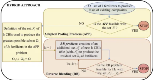
An Adaption of PP was designed, which we called ‘Adapted Pooling Problem’ (APP), that considers all the specificities of RB with the aim of creating as many CBIs as possible from existing composite materials, with the remaining CBIs having to be created as new composite materials.

4. Modelling

To clearly account for the differences and complementarities be-tween the Blending Problem (BP), the Reverse Blending problem (RB) and the Pooling Problem (PP), their mathematical formulation (x4.1 to

x4.3) must be examined. This led to an Adapted Pooling Problem (APP)

(x4.4), which induced a general approach, named Extended Reverse Blending (ERB), combining APP with RB (x4.5).

4.1. Blending problem Indexes and parameters

i Existing inputs (raw material or composite material) ði ¼ 1;:::;IÞ. j Output index ðj ¼ 1;:::;JÞ.

c Component index ðc ¼ 1;:::;CÞ/common to all models.

βmin_cj Minimal proportion weight of component c in the weight of

output j. βmax

cj Maximal proportion weight of component c in the weight of

output j.

Dj Demand for output j, expressed in weight.

Ai Availability of input i, expressed in weight.

αci Proportion of component c in the total weight of input i (raw

material or composite material).

ωi Unit cost of input i.

Variables

xij Quantity of input i used in the production of output j.

Problem definition Min X j X i ωi⋅xij ! (1) Subject to X i xij¼Dj; 8j (2) βmin cj � X i αci⋅xij , Dj�βmaxcj ; 8c; 8j (3) X j xij�Ai; 8i (4) Comments

� Relation (1): cost minimization.

� Relation (2): satisfaction of demand.

� Relation (3): satisfaction of composition constraints of an output.

� Relation (4): respect of input availabilities.

� Implicitly, the formulation is a mono-period one (steady state).

4.2. Reverse Blending problem (RBP)

As RBP aims to meet a potential demand for any fertilizer (without a priori market study), in RBP formulation, fertilizer demand must be conventional. In addition, specifications of inputs, whose blends pro-duce the required fertilizers, are to be defined. It follows that input costs are unknown at this stage, such that a formulation based on economic optimization would be pointless as neither demand nor costs are known. RBP only aims to find a feasible blending solution in a steady state for a set of fertilizers as well as the composition of the CBIs used, whose number must be as low as possible to reduce production, storage and transportation problems.

Indexes and parameters

j Becomes the index of a fertilizer.

i Becomes the index of a CBI, which is now a new composite ma-terial to be created, ði ¼ 2; :::; I’Þ where parameter ‘I’’ is the accept-able upper limit for the number of CBIs. Composite i ¼ 1 is the filler. c Component index ðc ¼ 1; :::; CÞ; only C ¼ 4 components are considered here; the filler is component c ¼ 4 .

Dj Becomes conventional demand for fertilizer j, expressed in Kg/

ha, needed to cover the nutrient requirements of a 1 ha plot of land.

β_cj Target proportion of component c in the total weight of output

(fertilizer) j.

η_cj Maximal absolute deviation of component c in the total weight

of output (fertilizer) j.

τci Maximal proportion weight of component c < 4in the total

weight of CBI i > 1 (see feature f in x3.4).

τ4i Minimal proportion weight of component c ¼ 4 (filler) in the

total weight of CBI i > 1.

αc1 The proportion of component c in the total weight of CBI i ¼ 1 .

For this CBI, which is filler, αc1¼0; 8c < 4 and α41¼1 (as the CBI

filler is 100% made of filler).

M Upper boundary of any CBI quantity used to produce an output (e.g., M ¼ 100000).

κ Minimal weight percentage of a CBI used to produce an output (a

fertilizer), if that CBI is used (e.g., κ ¼ 0:01Þ: Variables

xij Quantity of CBI i used in the production of fertilizer j.

αci Becomes the weight proportion of component c in the total

weight of CBI i > 1; note that in the blending problem, αci is a

the filler (implying that αc1 are parameters and not decision

variables).

wij Binary variable which is equal to1 if CBI i is used to produce

fertilizer j and 0 otherwise.

yi Binary variable which is equal to1 if CBI i is used and 0

other-wise. The set of I ¼Piyi inputs constitutes a Canonical Basis

enabling the production of any fertilizer. Problem definition Min " X i yi # (5) Subject to X i xij¼Dj; 8j (2a) X j xij�M⋅yi; 8i (6) � � � � � β_cj ηcj� X i αci⋅xij , Dj�βcjþηcj; 8c; j � � βcj>0 X i αci⋅xij , Dj¼0; 8c; j � � βcj¼0 (3a) X c αci¼1; 8i (7) � � � �α_αci�τci​ ; ​ 8i; cjc < 4 4i�τ4i; 8i (8) � � � �x_xij�M⋅wij ij�κ⋅wij⋅Dj; 8i; j (9) Comments

�Relation (5) defines the optimization criteria designed to obtain a

feasible solution (i.e., respecting relation 2, 3a and 7 to 9) where I ¼ P

iyi is as low as possible.

�Relation (6) enforces y_i to be equal to 1 only if CBI i is used; that said,

the objective function (5) aims to maximize the number of CBIs

unused (the set of CBIs i where yi ¼0) so as to keep I as small as

possible.

�Relations (3a) replace relation (3) while tolerating deviation η_cjfrom

the target values βcj when βcj>0. Clearly, (3a) is equivalent to (3)

when η_cj¼ ðβmax

cj βmincj Þ=2 and βcj¼βmincj þηcj , but this formulation is

chosen on account of fertilizer regulation (EU PE-CONS 76/18,

2019) which sets target values and tolerances unlike in the classical blending problems where the specifications are expressed as a min-max bracket. Due to relations (3a), the problem becomes a quadratic one.

�Relation (7) constrains the CBI composition to ensure the aggregate

of component proportion weights equals 100%.

�Relations (8) constrain the CBI nutrient proportion not to exceed its

maximal allowed value while having a minimum proportion of filler (see feature f in x3.4).

�Relations (9), which connect the continuous variables to the binary

ones, ensure that if CBI i is to be used to produce fertilizer j, it must represent at least κ% of this fertilizer’s weight.

4.3. Pooling problem (PP)

The formulation of the standard pooling problem proposed by Gupte

et al., (2017) is presented below. This standard version applies to network flow models consisting of arcs and nodes with capacity limit

constraints for both the nodes (tanks) and arcs (devices connecting different units). However, to make the distinction between PP and RB problem easier, this version was adapted to only retain the constraints representing similarities with a RB problem. That said, the limiting ca-pacity constraints are eliminated and the variable decisions now concern quantities and proportions instead of arc flows. Additionally, in PP problems, unlike in RBP, in addition to arcs connecting inputs to pools (intermediate blends) and pools to outputs, there are flows from inputs to outputs.

Indexes and parameters

I Number of pools (fixed value).

k Index of an existing raw materialðk ¼ 1;:::;KÞ.

i Becomes the index of an intermediate input to create ði ¼ 1;:::;IÞby blending raw materials.

j As in the BP, j is the index for an output (final blend)ðj ¼ 1;:::;JÞ.

φ_kj The cost of sending a unit flow on the arc connecting raw

ma-terial k to final blend j.

φ_ki The cost of sending a unit flow on the arc connecting raw

ma-terial k to intermediate input i.

φ_ij The cost of sending a unit flow on the arc connecting

interme-diate input i to final blend j.

γ_ck Proportion of component c in the total weight of raw materialk.

Ak Availability of raw material k, expressed in weight (replaces Ai

in the BP formulation).

Dj Becomes the maximum demand for j.

βmin

cj Minimal proportion weight of component c in the weight of

output j. βmax

cj Maximal proportion weight of component c in the weight of

output j. Variables

xij Becomes the quantity of intermediate input i used in the

pro-duction of output j.

αci Weight proportion of component c in the total weight of

inter-mediate input i.

yki Quantity of raw material k used in the production of

interme-diate input i.

zkj Quantity of raw material k sent directly to be used in the

pro-duction of output j. Problem definition Min X j;k ϕkj:zkjþ X k;i ϕki:ykiþ X i;j ϕij:xij ! (10) Subject to X i xijþ X k zkj�Dj; 8j (11) X j xij¼ X k yki; 8i (12) X j zkjþ X i yki�Ak; 8k (13) X k γck⋅ yki¼ ​αci⋅ X j xij; 8c; i (14) βmin jc � P k γckzkjþ P i αcixij � P k zkjþ P i xij � �β max jc ; 8​j; c (3b) Comments

�Relation (10): cost minimization.

�Relation (11) maximum withdrawal constraint (the sum of the

quantities of raw materials to be withdrawn zkj and/or intermediate

inputs xijmust not exceed demand Dj).

�Relation (12) flow conservation constraint of intermediate inputs.

�Relation (13) raw material availability constraint (the outgoing flows

from the raw material tanks, whether those going to the intermediate

tanks or the outputs tanks, must not exceedAk).

�Relation (14) flow conservation constraint of components.

�Relation (3b) variant of constraint (3) of output specifications taking

into account outflows from the pools and the raw material tanks. 4.4. Adapted pooling problem (APP)

After presenting the APP model (x4.4.1), an explanation of its reso-lution approach is given in x4.4.2.

4.4.1. APP formulation

In APP, one tries to use PP, as far as possible, to produce the

maximum number J1 of fertilizers obtained by blending I1 CBIs made

with existing composite materials that are assumed to be available. I1 is

a parameter that is gradually increased until reaching the possible highest value of J1(see x4.4.2).

Adaptation of the pooling formulation

k Becomes the index of an available composite material (instead of a raw material).

i Becomes the index of a CBI made by blending composite materials ði ¼ 1; :::; I1Þwhere I1 is a parameter to be adjusted (and not a fixed parameter, as in PP).

New parameters

ζ_kk0 Boolean parameter equal to 1 if composite materials k and k

0

are incompatible, and 0 otherwise.

κ’ Minimal weight percentage of a composite material k used to

produce a CBI, if that composite material is used.

ε Very low value (e.g., ε ¼0.00001).

New variables

vj Binary variable equal to1 if fertilizer j is produced and

0 otherwise.

zki Binary variable equal to1 if composite material k is used to

produce CBI i and 0 otherwise. Problem definition Max " X j vj # (15) Subject to X i xij¼Dj; 8j (2) � � � � � β_cj ηcj� X i αci⋅xij , Dj�βcjþηcj; 8c; j � � βcj>0 X i αci⋅xij , Dj¼0; 8c; j � � βcj¼0 (3a) � � � �xij �M⋅wij xij�κ⋅wij⋅Dj; 8i; j (9) � � � � � X i xij�M⋅vj X i xij�ε⋅vj ; 8j (16) X j xij¼ X k yki; 8i (12) � � � � � yki�M⋅zki yki�κ’⋅zki⋅ X j xij; 8k; i (17) zkiþzk0i�1 ; 8i; k; k 0 jk 6¼ k0^ ζ_kk0¼1 (18) wijþwi0j�3 ζkk0⋅ðzkiþzk0i’Þ; 8j; 8i; i 0 ji06¼i; 8k; k0jk 6¼ k0^ ζ_kk0¼1 (19) Comments

� Relation (15) maximizes the number of fertilizers that may be

pro-duced with I1 CBIs obtainable by blending existing composite

ma-terials; as I1 is a parameter that must be as low as possible, APP is a

parametric quadratic problem.

� Relation (2) is taken from BP while relations (3a) and (9) are taken

from RBP.

� Relations (16) enforce vj to be equal to 1 if fertilizer j is produced by a

blend of CBIs, otherwise to 0.

� Relation (12) is a flow conservation constraint taken from PP. In a

two-stage blending perspective, the previous relations deal with the first stage and the following ones, with the second stage.

� Relations (17) similar to relations (9) ensure z_ki¼1 ⇔ y_ki>0

(meaning composite material k is used to produce CBI i) and enforce the proportion of composite material k in the weight of CBI i to exceed a proportion κ’ (e.g.κ’ ¼ 1%), if composite material k is used to produce CBI i.

� According to feature b of x3.4, relation (18), aiming to prevent

blending incompatible composite materials in the CBI BOM, forbid the use of chemically incompatible mixtures when creating CBI granules. So, if for example the two composite materials k and k’ are

incompatible (i.e.ζkk0 ¼1), then these composites cannot be

com-bined in the blend producing CBI i (i.e.zkiþz_k0

i�1, zki being a binary

variable which is equal to 1 when composite k is used to produce CBI i). These incompatibilities are discussed in the dataset section (x5.1)

and illustrated in Table 3.

� According to feature b of x3.4, relation (19), aiming to prevent

blending incompatible CBIs in the fertilizer BOM, ensures compli-ance with the chemical incompatibilities inherited from the first blending stage when the CBIs are mixed to produce a fertilizer. Let

CBIs i and i’ respectively use composites k and k’ (involving zkiþ

zk0

i’¼2Þ, both CBIs being obtained by mixing compatible material

composites. Where these two composites are not compatible ðζkk0 ¼

1Þ, then CBIs i and i’ must not be combined in the production of any fertilizer j (involving: wijþw_i0

j�3 ðzkiþz_k0

i’Þ⇔wijþw_i0

j�1, wij

being a binary variable which is equal to 1 when CBI i is used to produce fertilizer j).

4.4.2. APP resolution

APP being a parametric quadratic problem where one searches the highest value of the fertilizers produced with a canonical basis of I1 CBIs

(quadratic feature) with the lowest possible value of I1 (parametric

feature), the following algorithm must be used to find the optimal

so-lution (optimal size I1 of the canonical basis and optimal fertilizer

blends, i.e.xij=Dj; 8j 2 Ω1;i 2 I1).

1 I1¼0

2 J*

1¼0 3 I1←I1þ1 (continued on next page)

(continued) 4 Solve the APP 5 If J1>J*1then 6 J* 1← J1 7 Go to 3 8 Else go to 9 9 Stop

4.5. Extended Reverse Blending (ERB)

This approach, summarized in Fig. 1, combines APP, whose solution

is a set I1 of I1 CBIs, made of existing composite materials, the blending

of which can produce the greatest set Ω1 of J1 fertilizers. Then, a RBP is

run to find the smallest set I 2 of new composite materials that

corre-sponds to I2 new CBIs which, combined with the initial set of CBIs, gives

a blending solution for the J2 remaining fertilizer requirements. In the

end, the specifications for all fertilizers Ω ¼ Ω1[Ω2 are satisfied.

5. The application

As explained in the introduction, the RB was tested on a sample of 700 fertilizer solutions. The aim was to find the minimum number of CBIs whose physical blending would successfully meet all 700 NPK re-quirements. The results of the RB models are presented in x5.2 before being discussed in x5.3.

5.1. Dataset

The 700 NPK requirements are given by Fertimap in Kg/ha. But as fertilizers are marketed in the form of percentage formulae, it is neces-sary to convert the quantitative NPK requirements into needs expressed in fertilizer formulae. Indeed, since any fertilizer contains a proportion of filler, this conversion was operated by setting the filler proportion. The idea was to do so in such a way as to obtain formulae that are similar to those of currently marketed fertilizers as this would facilitate their production using currently available composite materials. Accordingly, some 70 NPK fertilizers, listed in the catalogs of world leading fertilizer manufacturers, were analyzed. As a result, a set of 8 filler proportions was defined, resulting in 482 different formulae capable of matching Fertimap’s 700 NPK needs. These needs may be satisfied by other formulae of varying filler weight. Be that as it may, changing fertilizer formulae will not alter the approach. These formulae as well as demand

Dj for them, are presented in Table 2 for the NPK requirements listed in

Table 1. For example, to meet NPK requirement No. 362, 531.52 kg/ha of formula 26.03–4.90 21.07 must be applied. By multiplying these %

by the required quantity (531.52 kg/ha), we obtain respectively 138.33, 26.06 and 112 kg/ha of N, P and K which corresponds exactly to the

362nd _{NPK need. As explained at the end of x2.1, by excluding one-}

component fertilizers, the models are targeted on the remaining J ¼ 700 220 þ 2 ¼ 482 fertilizers. Using all 482 formulae, the RB and ERB solutions meeting all 700 NPK needs are listed.

Concerning input data of the RB problem relating to CBI composition constraints ensured by relation (8), the maximum proportions of N, P

and K in a CBI are set at τ1i¼46%;τ2i¼46% ​ and ​τ3i¼75% ​ ; 8i > 1

and the minimum proportion of filler at τ4i ¼5%. It is assumed that a

CBI must represent at least κ ¼ 1% of a fertilizer weight. For the toler-ated absolute deviation, a value of η_cj¼0:0003; 8c; j��c < 4 is used (which complies more than exceeds EU regulation requirements). For the APP input data, only the seven most important NPK material

com-posites in the fertilizer market are considered (see Table 3).

When ζkk’ ¼1, it is considered that composite materials k and k’ are

strictly incompatible. Yet, in practice, the blending of certain composite materials, forbidden above, can in fact, be tolerated subject to specific ratios depending on the composite material and ambient conditions. Since the exact values of these ratios are currently ignored (to be determined by experimentation), the limited incompatibilities are deemed to be strict. It is assumed that the industrial process used for CBI production requires, for any composite material k, a minimum propor-tion κ’ ¼ 1% for it to be used in the producpropor-tion of a CBI.

5.2. Results

The results below were produced by the Xpress solver using a PC (Intel® Xeon® CPU E3-1240 v5 @ 3.50 GHz - 64 Go RAM). Please note that this paper ignores RB computational efficiency aspects as at this stage of this research, the problem can be solved with commercial software. When dealing with much larger problems, computational ef-ficiency will of course be addressed. The results of RB and ERB are successively examined before discussing their results.

5.2.1. RB results

The application of the RBP model (see x4.2) to the above data set (variety of about seven hundred fertilizer solutions using about 482 different formulae) shows that only 8 CBIs are needed, including one

acting as filler (i ¼ 1) (see Table 4 and Reverse_Blending_results.xlsx,

included in the Mendeley data).

Table 5 contains an extract of the optimal quantities xij of these CBIs

to be withdrawn to meet demand for each fertilizer.

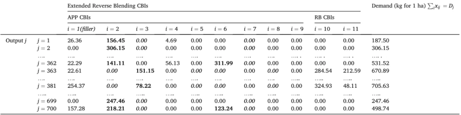
5.2.2. ERB results

First, with the APP model, the results determine the optimal CBIs,

that can be created from the composite materials of Table 3, which

maximizes the set of J1 producible fertilizers (J1¼626 fertilizers). These

626 can be obtained by compatible blends of just 9 CBIs (see the detail of the APP solution in the file Adapted_Pooling_results.xlsx, included in the Mendeley data). Then, the RBP model is used to define the remaining

optimal CBIs set that can be used, combined with the CBIs found with

APP, to produce the set Ω2 of J2 ¼74 remaining fertilizers. To this end,

only two additional CBIs must be created (i ¼ 10 and i ¼ 11) (see Table 6

and file Extended_RB_results.xlsx included in the Mendeley data).

An extract of the quantitiesxijof these CBIs to be withdrawn to

pro-duce each output j is presented in Table 7 while the quantities yki to be

withdrawn from each composite k to meet each CBI i are shown in Table 2

The composition ðβcjÞof the fertilizer formulae (outputs) and the demands ðDjÞ.

No. Need Geographical coordinates The specifications of the outputs

Longitude Latitude Output j The nutritional specifications ðβcjÞ Demands ðDjÞ(kg for 1 ha)

%N %P %K %Filler 1 7.9447 33.4608 j ¼ 1 38.84% 1.16% 0.00% 60.00% 187.50 2 7.9369 33.4561 j ¼ 2 46.00% 0.00% 0.00% 54.00% 306.15 … … … … 362 6.168 33.7713 j ¼ 362 26.03% 4.90% 21.07% 48.00% 531.52 363 5.9531 34.0845 j ¼ 363 29.41% 16.59% 24.00% 30.00% 670.89 … … … … 381 5.1789 34.7444 j ¼ 381 11.24% 11.65% 23.10% 54.00% 705.63 … … … … 699 4.4452 33.9143 j ¼ 699 46.00% 0.00% 0.00% 54.00% 247.46 700 4.3941 33.9137 j ¼ 700 25.13% 0.00% 8.87% 66.00% 498.74 Table 3

Composition of composite materials (γck) and their incompatibilities matrix (ζkk’). Composite material k

Filler Urea TSP KCl MAP DAP Potas. nitrates

k ¼ 1 k ¼ 2 k ¼ 3 k ¼ 4 k ¼ 5 k ¼ 6 k ¼ 7

Composition of the composite materials (γck)

Component c %N c ¼ 1 0 46 0 0 11.2 18.3 13.0

%P c ¼ 2 0 0 46 0 55.0 46.4 0

%K c ¼ 3 0 0 0 60 0 0 46.0

% Filler c ¼ 4 100.0 54.0 54.0 40.0 33.8 35.3 41.0

Matrix of the composite materials incompatibilities (ζkk’)

Composite material k Filler k ¼ 1 0 0 0 0 0 0 0

Urea k ¼ 2 0 0 1 1 0 0 0 TSP k ¼ 3 0 1 0 0 0 0 0 KCl k ¼ 4 0 1 0 0 0 0 0 MAP k ¼ 5 0 0 0 0 0 0 0 DAP k ¼ 6 0 0 0 0 0 0 0 Potas. Nitrates k ¼ 7 0 0 0 0 0 0 0 Table 4

Optimal composition of RB CBIs (αci).

CBI i i ¼ 1(filler) i ¼ 2 i ¼ 3 i ¼ 4 i ¼ 5 i ¼ 6 i ¼ 7 i ¼ 8 Component c %N c ¼ 1 0 46 0 22.53 29.78 12.83 52.20 20.32 %P c ¼ 2 0 0 46 0.15 23.53 0 42.32 0.49 %K c ¼ 3 0 0 0 0 0 47.09 0.49 74.19 % Filler c ¼ 4 100 40 50 77.31 46.69 40.08 5 5 Table 5

The optimal quantities to be withdrawn from the RB CBIs (xij).

CBI i Demand (kg for 1 ha) Pixij¼Dj

i ¼ 1(filler) i ¼ 2 i ¼ 3 i ¼ 4 i ¼ 5 i ¼ 6 i ¼ 7 i ¼ 8 Output j j ¼ 1 0.00 127.53 0.00 51.05 8.92 0.00 0.00 0.00 187.50 j ¼ 2 0.00 306.15 0.00 0.00 0.00 0.00 0.00 0.00 306.15 …. …. …. …. …. …. …. …. …. …. j ¼ 362 154.75 166.41 0.00 0.00 0.00 0.00 59.80 150.56 531.52 j ¼ 363 156.84 38.20 0.00 0.00 0.00 0.00 260.52 215.31 670.89 ….. ….. …. …. ….. ….. ….. ….. ….. ….. j ¼ 381 304.62 0.00 115.12 0.00 0.00 0.00 66.60 219.29 705.63 ….. ….. ….. ….. ….. ….. ….. ….. ….. ….. j ¼ 699 0.00 247.46 0.00 0.00 0.00 0.00 0.00 0.00 247.46 j ¼ 700 158.54 246.25 0.00 0.00 0.00 93.95 0.00 0.00 498.74

Table 8.

Table 7 shows that the CBIs were used in minimum quantities of

0:01 � Dj Kg/ha and that the inheritance of the incompatibilities, forced

by relation (19), was taken into account (e.g., as urea is not compatible

with TSP ðζ2;3¼1Þ, when a CBI which is made from TSP is used (case of

CBI 3), CBIs made from urea (CBIs 2, 5, 6 and 8) are excluded and vice versa). The bold/italic font is used to emphasize the fact that if a CBI i is used (written in bold), then the quantity to be extracted from the inputs that are incompatible with this CBI i is zero (written in italic).

Table 8 shows that the quantities yki all correspond to 100% of the

total quantity required for each CBI ðPkyki¼P_jx_ijÞ thus satisfying

relation (12). Also, thanks to relation (17), the minimum proportion κ’

set at 1% for all the composites as well as the incompatibilities of Table 3

were taken into account. 6. Discussion

In addition to the filler, RB came up with 7 CBIs whose possible combination fully satisfies the 700 NPK requirements. Besides accu-rately delivering the exact nutritional requirements, this drives huge flow massification by reducing the flows to be managed from 100% to just 1.57% (subject to laboratory experiments finding chemically stable reactions for the development of these new formulae). Otherwise, if a CBI technical feasibility is to be achieved by blending available compatible composite materials (through the APP), then the number ‘I’ of CBIs may increase slightly. Indeed, using the ERB hybrid approach, the number of the required CBIs went up from 7 (possibly unfit for manufacturing) CBIs (standard RB) to 10 CBIs (extended RB) (see Table 6) which are known to yield eight feasible formulae. In both cases, 700 fertilizer solutions can be provided with no more than 10 CBIs.

With such a disruptive solution, which as yet to be implemented, no benchmark is possible with any fertilizer company. Nevertheless, if one takes the real life example of 700 fertilizer needs, involving 482 different fertilizers formulas, it is obvious that no fertilizer plant can achieve annual production to stock (or to order) of at least 482 batches of these fertilizers, involving as many setups (each requiring around 2 h) and

solve the associated problems of separate storage and transportation. The results show that these requirements can be met with a canonical basis of 8 new inputs with Reverse Blending (or 11, with Extended Reverse Blending). Clearly, this flow massification drastically reduces the issues confronting fertilizer plants. These are such that currently they are able to cope at best with a diversity of a few dozens of different fertilizers (for example, the world’s ten largest fertilizer companies offer a variety of less than 180 different fertilizers). It can be argued that the proposed solution involves remote blending, and thus additional costs. To this, it can be answered that remote blending of fertilizers is already done in some countries, with very poor results, as it is limited to a mix of two or three existing fertilizers, which hardly satisfies all nutrient requirements.

After showing that a feasible solution ensuring maximum flow massification may be found, we outline in the conclusion the next steps of this research.

7. Conclusion

Reverse Blending appears to be an economically efficient way of delivering customized fertilizers that satisfy the needs of sustainable agriculture while reducing production and transportation costs and is-sues thanks to flow consolidation (as detailed in x2.2). This, however, involves reengineering the production and distribution processes, which means that industries wishing to implement RB must be prepared to redesign their supply chain. RB, therefore, forms part of a long-term strategy with a predictable impact on the supply chain. Indeed, flow consolidation will deliver multiple streamlining opportunities such as increasing production capacity, reducing storage problems and avoiding shipping costs and problems. While the potential interest of the RB approach may be obvious, a number of issues still need to be addressed: implementing the approach requires the expertise of a multidisciplinary team. Bringing scientists from a variety of different backgrounds together is a crucial part of fixing the world’s problems especially when it comes to projects that involve multiple scientific disciplines. Table 6

Optimal composition of the hybrid extended RB CBIs (αci).

Extended Reverse Blending: CBI i to be obtained with

The existing composite materials (Result of the APP model) New composite materials to be created (Result of

the RB model) i ¼ 1(filler) i ¼ 2 i ¼ 3 i ¼ 4 i ¼ 5 i ¼ 6 i ¼ 7 i ¼ 8 i ¼ 9 i ¼ 10 i ¼ 11 Component c %N c ¼ 1 0 46 0 18.30 37.05 20.25 12.64 31.27 12.60 13.31 75 %P c ¼ 2 0 0 46 46.40 15 0 0 22.23 2.64 14.12 0.75 %K c ¼ 3 0 0 0 0.00 0 35.90 46.39 0 42.67 48.58 10.71 % Filler c ¼ 4 100 54 54 35.30 47.95 43.86 40.97 46.50 42.09 23.99 13.54 Table 7

Optimal quantities required for ERB CBIs (xij).

Extended Reverse Blending CBIs Demand (kg for 1 ha) Pixij¼Dj

APP CBIs RB CBIs

i ¼ 1(filler) i ¼ 2 i ¼ 3 i ¼ 4 i ¼ 5 i ¼ 6 i ¼ 7 i ¼ 8 i ¼ 9 i ¼ 10 i ¼ 11 Output j j ¼ 1 26.36 156.45 0.00 4.69 0.00 0.00 0.00 0.00 0.00 0.00 0.00 187.50 j ¼ 2 0.00 306.15 0.00 0.00 0.00 0.00 0.00 0.00 0.00 0.00 0.00 306.15 …. …. …. …. …. …. …. …. …. …. . …. . …. . …. . j ¼ 362 22.29 141.11 0.00 56.13 0.00 311.99 0.00 0.00 0.00 0.00 0.00 531.52 j ¼ 363 22.61 0.00 151.15 0.00 0.00 0.00 0.00 0.00 0.00 284.54 212.59 670.89 …. …. …. …. …. …. …. …. …. ….. ….. ….. ….. j ¼ 381 254.37 0.00 78.22 0.00 0.00 0.00 0.00 0.00 0.00 324.93 48.11 705.63 ….. ….. …. ….. ….. ….. ….. ….. ….. ….. ….. ….. ….. j ¼ 699 0.00 247.46 0.00 0.00 0.00 0.00 0.00 0.00 0.00 0.00 0.00 247.46 j ¼ 700 157.28 218.21 0.00 0.00 0.00 123.24 0.00 0.00 0.00 0.00 0.00 498.74

In bold: the non-zero quantities that are taken from the used CBIs. In italic: the “0” (zero quantities) corresponding to CBIs that are unused because of their in-compatibility with the used CBIs (the ones in bold).

�First, agronomists should be asked to define the exact nutrient re-quirements for land parcels across countries. These rere-quirements depend on the “soil/crop” combinations and their identification re-quires state-of-the art agronomic expertise. Additionally crops will range from the current ones to those that are targeted by local policy.

�Secondly, chemists shall be called upon to further expand the

com-posite materials set, address the assumptions (mentioned at the end of §5.1) used to simplify the constraints related to composite mate-rials incompatibilities and eventually experiment and study the sta-bility of new chemical reactions that would be essential for the new formulae to be designed.

�Thirdly, it is planned to work on large projects and study the impact

of this transformation of production processes on OCP’s supply chain (our sponsor) and eventually design new distribution and production schemes. These will be based on several scenarios describing the impact on transport of massive flow consolidation as well as the nature, location and sizing of post-manufacturing blending facilities to be installed in Africa, one of OCP’s largest markets.

To conclude, RB may be used by other industries, like cosmetics, which is well on its way to marketing 100% customized products. Lastly, with reference at least to the fertilizer sector, RB effectiveness does not boil down to achieving corporate goals but, more importantly, appears to be a major lever in solving the looming food supply crises facing mankind and, as such, clearly belongs to the field of corporate social responsibility.

Data Set and Results are included in the Mendeley data (https://doi.

org/10.17632/z3sbn5j9z7.1) Credit author statement

Latifa Benhamou: Conceptualization, Methodology, Software, Vali-dation, Formal analysis, Investigation, Resources, Writing - Original Draft, Visualization, Vincent Giard: Conceptualization, Methodology, Validation, Formal analysis, Investigation, Writing - Review & Editing, Visualization, Supervision, Mehdi Khouloud: Validation, Resources, Pierres Fenies: Supervision, Fr�ed�eric Fontane: Supervision, Project administration, Funding acquisition

References

Adhya, N., Tawarmalani, M., Sahinidis, N.V., 1999. A Lagrangian approach to the

pooling problem. Ind. Eng. Chem. Res. 38, 1956–1972. https://doi.org/10.1021/

ie980666q.

Akkerman, R., Van Der Meer, D., Van Donk, D.P., 2010. Make to stock and mix to order: choosing intermediate products in the food-processing industry. Int. J. Prod. Res. 48,

3475–3492. https://doi.org/10.1080/00207540902810569.

Alaoui, S.B., 2005. R�ef�erentiel pour la Conduite Technique de la Culture du bl�e dur (Triticum durum) 14.

Aldeseit, B., 2014. Linear programming-based optimization of synthetic fertilizers

formulation. J. Agric. Sci. 6 https://doi.org/10.5539/jas.v6n12p194.

Alfaki, M., 2012. Models and Solution Methods for the Pooling Problem. The University of Bergen.

AlGeddawy, T., ElMaraghy, H., 2010. Assembly systems layout design model for delayed

products differentiation. Int. J. Prod. Res. 48, 5281–5305. https://doi.org/10.1080/

00207540903117832.

Anderson, D.M., Pine II, B.J., 1997. Agile Product Development for Mass Customization: How to Develop and Deliver Products for Mass Customization Niche Markets, JIT, Build-To-Order and Flexible Manufacturing. McGraw-Hill.

Ashayeri, J., van Eijs, A.G.M., Nederstigt, P., 1994. Blending modelling in a process

manufacturing: a case study. Eur. J. Oper. Res. 72, 460–468. https://doi.org/

10.1016/0377-2217(94)90416-2.

Audet, C., Brimberg, J., Hansen, P., Digabel, S.L., Mladenovi�c, N., 2004. Pooling problem: alternate formulations and solution methods. Manag. Sci. 50, 761–776. https://doi.org/10.1287/mnsc.1030.0207.

Babcock, B., Rister, M.E., Kay, R.D., Wallers, J.A., 1984. Identifying least-cost sources of

required fertilizer nutrients. Am. J. Agric. Econ. 66, 385–391. https://doi.org/

10.2307/1240806.

Baud-Lavigne, B., Agard, B., Penz, B., 2012. Mutual impacts of product standardization

and supply chain design. Int. J. Prod. Econ. 135, 50–60. https://doi.org/10.1016/j.

ijpe.2010.09.024.

Bengtsson, J., Bredstr€om, D., Flisberg, P., R€onnqvist, M., 2013. Robust planning of blending activities at refineries. J. Oper. Res. Soc. 64, 848–863.

Bilgen, B., Ozkarahan, I., 2007. A mixed-integer linear programming model for bulk

grain blending and shipping. Int. J. Prod. Econ. 107, 555–571. https://doi.org/

10.1016/j.ijpe.2006.11.008.

Boone, C.A., Craighead, C.W., Hanna, J.B., 2007. Postponement: an evolving supply

chain concept. Int Jnl Phys Dist & Log Manage 37, 594–611. https://doi.org/

10.1108/09600030710825676.

Bown, H.E., Watt, M.S., Clinton, P.W., Mason, E.G., 2010. Influence of ammonium and nitrate supply on growth, dry matter partitioning, N uptake and photosynthetic

capacity of Pinus radiata seedlings. Trees 24, 1097–1107. https://doi.org/10.1007/

s00468-010-0482-1.

Chang, J.C., 2015. Designing Two-Stage Recycling Operations for Increased Usage of Undervalued Raw Materials (Thesis). Massachusetts Institute of Technology. Chang, J.C., Graves, S.C., Kirchain, R.E., Olivetti, E.A., 2019. Integrated planning for

design and production in two-stage recycling operations. Eur. J. Oper. Res. 273,

535–547. https://doi.org/10.1016/j.ejor.2018.08.022.

Cheng, X., Tang, K., Li, X., 2018. New multi-commodity flow formulations for the

generalized pooling problem. IFAC-PapersOnLine 51, 162–167. https://doi.org/

10.1016/j.ifacol.2018.09.293.

Cole, B.M., Bradshaw, S., Potgieter, H., 2015. An optimisation methodology for a supply chain operating under any pertinent conditions of uncertainty - an application with two forms of operational uncertainty, multi-objectivity and fuzziness. Int. J. Oper. Res. 23, 200–227.

Conforti, P., Sarris, A.S., 2012. Challenges and Policies for the World Agricultural and Food Economy in the 2050 Perspective, pp. 509–540. FAO (chapter 12). Cottenie, A., 1980. Soil and plant testing as a basis of fertilizer recommendations. FAO

Soils Bull. 38 (2).

Daaboul, J., Da Cunha, C.M., 2014. Differentiation and customer decoupling points: key value enablers for mass customization. In: Grabot, B., Vallespir, B., Gomes, S., Bouras, A., Kiritsis, D. (Eds.), Advances in Production Management Systems. Innovative and Knowledge-Based Production Management in a Global-Local World.

Springer Berlin Heidelberg, Berlin, Heidelberg, pp. 43–50. https://doi.org/10.1007/

978-3-662-44733-8_6.

Davis, S.M., 1989. From “future perfect”: mass customizing. Planning Review. https://

doi.org/10.1108/eb054249.

Epstein, E., Bloom, A.J., 2005. Mineral nutrition of plants : principles and perspectives. In: Sunderland, Mass. ; [Great Britain], second ed. Sinauer Associates.

Table 8

Optimal quantities yki required for each composite k.

APP RB Pjxij

filler Urea TSP KCl MAP DAP Potassium nitrates Pkyki k ¼ 1 k ¼ 2 k ¼ 3 k ¼ 4 k ¼ 5 k ¼ 6 k ¼ 7

APP CBI i i ¼ 1 (filler) 40,562.06 0.00 0.00 0.00 0.00 0.00 0.00 40,562.06 ¼ 40,562.06

i ¼ 2 0.00 108,230.83 0.00 0.00 0.00 0.00 0.00 108,230.83 ¼ 108,230.83 i ¼ 3 0.00 0.00 5623.60 0.00 0.00 0.00 0.00 5623.60 ¼ 5623.60 i ¼ 4 0.00 0.00 0.00 0.00 0.00 49,659.79 0.00 49,659.79 ¼ 49,659.79 i ¼ 5 0.00 5044.22 0.00 0.00 0.00 2409.66 0.00 7453.88 ¼ 7453.88 i ¼ 6 0.00 2701.88 0.00 0.00 0.00 0.00 9598.68 12,300.55 ¼ 12,300.55 i ¼ 7 0.00 0.00 0.00 48.92 0.00 0.00 1726.20 1775.12 ¼ 1775.12 i ¼ 8 17.54 270.32 0.00 0.00 0.00 264.82 0.00 552.68 ¼ 552.68 i ¼ 9 135.46 0.00 0.00 0.00 266.84 0.00 5153.16 5555.45 ¼ 5555.45 RB CBI i i ¼ 10 13,703.54 ¼ 13,703.54 i ¼ 11 7948.44 ¼ 7948.44

In bold: the non-zero quantities that are taken from the used composites. In italic: the “0” (zero quantities) corresponding to composites that are unused because of their incompatibility with the used composites (the ones in bold).