The Role of Fixed Cost in International
Environmental Negotiations
Basak BAYRAMOGLU &Jean-François JACQUES
yzNovember 10, 2010
Abstract
We investigate the relative e¢ ciency of an agreement based on a uniform standard without transfers and one based on di¤erentiated standards with transfers when strictly identical countries deal with transboundary pollution. We especially ask what role …xed cost plays.
INRA, UMR Economie Publique; AgroParisTech. Address: Avenue Lucien Brétignières, 78850 Thiverval Grignon, France. Tel: (0)1 30 81 45 35, E-mail: [email protected].
yLEDa, Université Paris-Dauphine, Place du Maréchal de Lattre de Tassigny, 75016
Paris. Tel: (0)1 44 05 44 60, E-mail: [email protected].
zWe gratefully acknowledge Bernard Caillaud and the three anonymous referees for
their comments. We are particularly indebted to one referee who o¤ered numerous, par-ticularly constructive insights. Brian Copeland, Maia David and Stéphane de Cara also made helpful suggestions. We thank the participants of the European Summer School in Resource and Environmental Economics, Venice (July 2004) and the EUREQua-Université Paris 1 seminar, Paris (September 2004) for comments, and S. Tanis-Plant for fruitful dis-cussions and editorial advice in English. This work was initiated during a research visit at the University British Columbia (Vancouver). We therefore also thank Ivar Ekeland for giving us that opportunity. Any errors are the responsibility of the authors.
Two approaches are examined: the Nash bargaining solution, impli-cating two countries, and the coalition formation framework, implicat-ing numerous countries and emphasizimplicat-ing self-enforcimplicat-ing agreements. In the former, in terms of welfare, strictly identical countries may wish to reduce their emissions in a non-uniform way under the di¤erenti-ated agreement. For this result to hold, the …xed cost of investment in abatement technology must be su¢ ciently high. The nature of the threat point of negotiations, however, also plays a crucial role. As concerns global abatement, the two countries abate more under the uniform agreement than under the di¤erentiated one. In terms of coalition formation when numerous countries are involved, a grand coalition could emerge under a di¤erentiated agreement.
Keywords: transboundary pollution, bargaining, standards, trans-fers, …xed cost, coalition stability.
JEL: Q50, C71.
Summary: In this paper, a situation in which identical countries faced with a transboundary pollution problem is investigated. All countries are re-sponsible for this pollution and seek to …nd an institutional arrangement in order to reduce it. We study the relative e¢ ciency of an agreement based on a uniform standard without transfers and an agreement based on di¤erenti-ated standards with transfers when two strictly identical countries are dealing with a problem of transboundary pollution. In the case of a uniform agree-ment, both countries abate and pay the …xed cost of abatement. In the case
of a di¤erentiated agreement, only one of the two countries would abate and pay for the …xed cost of investment. In return, its e¤orts would be com-pensated by monetary transfers. This analysis is carried out using the Nash bargaining solution (Nash (1950)) which makes it possible to determine the equilibrium of a negotiation game implicating two countries. Fixed cost, being part and parcel of abatement technology, plays a major role in determining the relative e¢ ciency of these two types of agreement. We reveal that above a threshold level of …xed cost, the countries may prefer to sign the di¤erentiated agreement, rather than the uniform one. The nature of the threat point of negotiations, however, also plays a crucial role. Furthermore, we show that the two countries abate more under the uniform agreement than under the di¤erentiated one. When this problem is tackled in terms of self-enforcing agreements for numerous countries, a grand coalition could emerge in the case of a di¤erentiated agreement.
1
Introduction
A situation in which similar countries facing the challenge of a transboundary pollution problem comes under study. Each country is both the cause and the victim of this pollution problem. The countries are identical in terms of abatement costs and their willingness to pay for cleaning up the environment they share. They are seeking an institutional arrangement in order to tackle this problem.
This institutional arrangement, in our case, is an International Environ-mental Agreement (hereafter referred to as an IEA). Such an agreement is based on an abatement standard: this is de…ned as the reduction of current emissions in order to reach a percentage of the emissions of a base year. In this case, the countries could choose one standard from a set of two: either a uniform standard or a di¤erentiated standard. The uniform standard means that the above-mentioned percentage would be the same for any country signing an agreement. The Montreal Protocol on Substances that Deplete the Ozone Layer fell into this category of agreements. It included a provision which speci…ed a reduction of emissions of CFCs (Chloro‡uorocarbons) and halons by 20 percent based on 1986 emission levels, to be accomplished by
1998 (Finus (2001), chapter 11).1 The di¤erentiated standard means that
the percentages would be di¤erent according to the country. The Kyoto Protocol on Climate Change (1997) and the Oslo Protocol on Further
Re-1Another example is the Helsinki Protocol (1985) which suggested a reduction of
duction of Sulphur Emissions (1994) are both examples of agreements with di¤erentiated standards.
Within the context a transboundary pollution problem across identical countries, we further de…ne a uniform agreement to be the case where there is reciprocal action. This means that each country undertakes the same abate-ment e¤ort, and any country involved pays for the …xed cost of investabate-ment in the abatement. This uniform abatement is a cost-e¤ective solution given that the countries under study are identical. We call this undertaking an agreement based on a uniform standard without transfers or in short a uni-form agreement. Since countries are identical, there is no need for a transfer payment scheme. We next de…ne a di¤erentiated agreement to be the case where there is unilateral action. This means that only some of the countries opt to make an abatement e¤ort, and pay for the …xed cost, while any other
countries compensate with transfers.2 We refer to this undertaking as the
agreement based on di¤erentiated standards with transfers or in short the di¤erentiated agreement.
In this paper, we emphasize the role of environmental protection …xed costs, which are part and parcel of abatement technology, for the outcome of international environmental negotiations. The recent environmental coop-eration around the regional pollution problem in the Mediterranean Sea can
2Transfer payments are o¤ered in order to increase participation in IEAs. Some
exam-ples of IEAs which include the possibility of transfers between countries are the Fur Seal Treaty (1911), the Montreal Protocol (1987), and the Stockholm Convention on Persistent Organic Pollutants (2001). See respectively Barrett (2003, p.34), Barrett (2003, p.346), and http://chm.pops.int/default.aspx for more details.
serve as an example. The Mediterranean Hot Spot Investment Programme (MeHSIP) and the Horizon 2020 initiative constitute the base of the Eu-ropean Union’s cooperation with the southern and eastern Mediterranean countries. The objective of MeHSIP is to abate 80 % of Mediterranean pol-lution by 2020. To help countries to undertake investment projects, the Programme foresees several …nancing mechanisms, both bilateral and
mul-tilateral. The report provided by the Programme Horizon 20203 states that
“Especially as concerns hazardous wastes, very little has been done so far in the MENA [Middle East and North Africa] countries to take care of this issue, the main reason for this being the high costs of the necessary investments e.g. incineration plants.” (p.30). The high …xed installation cost of these plants represents some of the investment costs of the projects …nanced by MeHSIP. It is clear from this example that the abatement of hazardous wastes in these countries would not take place without MeHSIP’s funding. As this example, among others, displays, the level of …xed costs in abatement technology can play a role in the outcome of international environmental negotiations.
In this paper, we ask what role …xed cost plays. Given the agreements (uniform agreement and di¤erentiated agreement) as we have de…ned them, more speci…cally, we investigate their relative e¢ ciency. To conduct this analysis, we examine two di¤erent approaches. Firstly, we adopt the Nash bargaining solution (Nash (1950)) as an equilibrium of a negotiation game implicating two countries. The threat point of negotiations is represented
by Nash equilibrium. We will show that three types of Nash equilibria can emerge depending on the level of …xed cost. Secondly, we work within the coalition formation framework, implicating thereby numerous countries and emphasizing self-enforcing agreements. We extend the model provided by Barrett (1994) by including …xed costs in the abatement technology. Here, we assume that signatories simply maximize their joint welfare, whereas non-signatories individually play Nash equilibrium strategies. We then ask if the di¤erentiated agreement could lead to a larger number of signatories than the uniform one.
A considerable amount of literature focuses on the possible explanations
for why uniform standards prevail in the presence of asymmetric agents.4
In general, unless the countries are similar, uniform standards are less ‡exi-ble, and therefore less e¢ cient than di¤erentiated standards (Harstad (2007), p.2).5 However, studies show that in the case of IEAs, uniform standards are
frequently the case (Hoel (1991), p.64; Harstad (2007), p.2). The following arguments are put forward to explain this frequency: the stability of agree-ments argument (Finus and Rundshagen (1998)), the monetary transfers argument (Bayramoglu and Jacques (2005)) and the trade theory argument
4One can …nd in the literature several arguments explaining the use of uniform
stan-dards: the fairness argument (Welsch (1992)), the informational problems argument (Lar-son and Tobey (1994), Harstad (2007)), the “focal point”argument (Schelling (1960)), the agency problems argument (Boyer and La¤ont (1999)).
5If the countries have di¤erent marginal implementation costs, then uniform standards
will increase the total cost of attaining a given environmental objective (Hoel (1992), p.142). In an earlier work, Kolstad (1987) showed that the e¢ ciency losses associated with uniform environmental regulations increase when marginal bene…t and cost functions become more steeply sloped.
(Copeland and Taylor (2005)). Finus and Rundshagen (1998) show, in a coalition model, that for global pollutants, governments will decide on an agreement based on a uniform percentage reduction of emissions (known as the quota regime) rather than an agreement based on a uniform tax (known as the tax regime). In the tax regime, countries’net bene…ts are unevenly dis-tributed. In contrast, the quota regime distributes net bene…ts more in line with the countries’characteristics, as abatement depends on initial emission levels. Bayramoglu and Jacques (2005) show, in a negotiation game impli-cating two countries, the possible Pareto superiority of an agreement based on a uniform standard with transfers compared to an agreement based on di¤erentiated standards. The intuition in that case was that if it is less ex-pensive to make transfers payments across the countries in order to incite the country, which bene…ts less from global abatement but has lower abatement costs to abate, then it is in the interest of both of the countries to sign the uniform agreement. The argument behind the Copeland and Taylor (2005) trade model is that trade in goods can act as a substitute for trade in emis-sion permits. Therefore, uniform emisemis-sion reductions in a world with freely traded goods can be e¢ cient, even if trade in permits is banned.
Our paper di¤ers from the literature in that it focuses on a distinct issue. Our interest lies in the analysis of whether or not di¤erentiated standards can be optimal for perfectly symmetric countries. McAusland (2005) uses, with a similar aim in mind, a political economy model to highlight the possi-ble ine¢ ciency of uniform environmental regulations for identical countries.
McAusland shows that the harmonization of these regulations across jurisdic-tions could be negative for both the environment and global welfare, despite the countries being identical in all respects. This happens when politicians are captured by “dirty” industries and if the local e¤ects of damages are su¢ ciently large. The former condition results in weak environmental pol-icy. The latter condition makes the policy harmonization less e¤ective in internalizing pollution, and also leads to a lower harmonized environmental standard. These two e¤ects are detrimental for the environment and in turn for global welfare. By taking into account …xed cost in abatement technology, in the Nash-bargaining setting for two countries, we show that the uniform agreement is positive for the global environment, but it can be negative for the welfare of countries. In the coalition formation framework, implicating numerous countries, the uniform agreement can lead to a lower coalition size than the di¤erentiated one.
The paper is organized as follows. Section 2 presents the negotiation model based on the Nash-bargaining approach implicating just two coun-tries. The threat point of negotiations, the uniform agreement and the dif-ferentiated agreement are analyzed respectively, with the comparison of the individual welfare of each country across the agreements. Section 3 provides an extension of the model within the coalition formation framework, implicat-ing thereby numerous countries and emphasizimplicat-ing self-enforcimplicat-ing agreements in the case of the two institutional arrangements described above. Finally, in Section 4 we discuss our …ndings in terms of the level of …xed cost, individual
welfare and self-enforcing agreement.
2
The Model
The utility function of country i = 1; 2 is written as follows:
N Bi = B(ai+ a i) C(ai) (1)
where ai is the individual abatement level of country i = 1; 2:
The bene…ts from global abatement are represented by the function B(ai+a i);assumed to be increasing and concave. For simplicity, we assume
that B(0) = 0:
The abatement costs are represented by the function C(ai) = co+ c(ai);
when ai is strictly positive. This function is composed of a …xed cost co and
a variable cost c(ai). The variable cost function is assumed to be increasing
and convex. We assume that the total cost of a country is zero when it does not abate, i.e., C(ai) = 0 when ai = 0 for i = 1; 2.
Throughout the paper, we will illustrate our theoretical results by an example with quadratic bene…t and cost functions. The chosen functional
forms are the following: B(x) = x 2x2 with x < ; and c(x) =
2x 2:
Parameters ; and are assumed to be strictly positive.
In this paper, we compare the abatement and welfare levels under the agreement based on a uniform standard without transfers, hereafter denoted
as U, and the agreement based on di¤erentiated standards with transfers, hereafter denoted as DT. Agreement U implies the same level of abatement
for the countries (ai = a i), whereas agreement DT allows di¤erent levels
of abatement (ai = 0 and a i 6= 0 or, ai 6= 0 and a i = 0). Moreover,
under this agreement, the country which undertakes an abatement e¤ort and pays for the …xed cost of investment receives transfer payments from the other country (t > 0). A question arises: is there a threshold level of …xed cost above which the DT agreement is better for each country than the U agreement? We shall show that it is not obviously so.
Before analyzing the outcome of the negotiations, we …rst study the non-cooperative equilibrium of the game, which constitutes the threat point in the negotiations.
2.1
Non-cooperative Equilibria
The non-cooperative game is represented here by Nash equilibrium. The objective of each country is to maximize its utility function by taking the abatement level of the other country as given:
M ax
ai
N Bi = M axai[B(ai+ a i) co c(ai)] (2)
We will show that two threshold levels of …xed cost co1 and co2 de…ne
1. For co < co1: each country abates (Type 1 symmetric Nash equilibrium)
2. For co1 < co < co2: only one country (say country 1) abates (Type 2
asymmetric Nash equilibrium)
3. For co > co2: no country abates (Type 3 symmetric Nash equilibrium)
We now de…ne the levels of abatement and the above mentioned threshold levels of …xed cost which limit the range of each type of Nash equilibrium.
Lemma 1: Letba be the abatement of each country at Type 1
sym-metric Nash equilibrium. It is characterized in the following way: B0(2ba) =
c0(ba).
Let bba be the abatement of country 1 at Type 2 asymmetric Nash equilib-rium. It is characterized in the following way: B0(bba) = c0(bba):
Proof: see proof Proposition 1.
Lemma 2: Let co1 be the threshold level of …xed cost below which
each country abates at Type 1 symmetric Nash equilibrium: co1 is equal to
B(2ba) c(ba) B(bba).
Let co2 be the threshold level of …xed cost above which no country abates
at Type 3 symmetric Nash equilibrium: co2 is equal to B(bba) c(bba):
Proof: see proof Proposition 1.
Lemma 3: co1 < co2:
Proof. The function 2B(x) c(x) is concave. It attains its maximum
that x is higher than bba, because 2B0(bba) c0(bba) = B0(bba) > 0. We also
know that bba is higher than ba, because B0(ba) > B0(2ba) = c0(ba). This implies
that B0(ba) c0(ba) > 0. Consequently, 2B(x ) c(x ) > 2B(bba) c(bba) >
2B(ba) c(ba) > B(2ba) c(ba): The …nal inequality is related to the concavity of the function B(:) which implies that 2B(x) > B(2x) (with B(0) = 0: If
not, we would consider the function (B(x) B(0))and obtain an equivalent
result).
Proposition 1 presents the general conditions under which the three Nash equilibria exist.
Proposition 1: If 0 < co < co1; then the equilibrium is a Type
1 symmetric Nash equilibrium with the following levels of utility for each country,
N B1 = N B2 = B(2ba) co c(ba):
If co1 < co < co2;then the equilibrium is a Type 2 asymmetric Nash
equi-librium with the following levels of utility for the countries,
N B1 = B(bba) co c(bba); NB2 = B(bba):
If co > co2; then the equilibrium is a Type 3 symmetric Nash equilibrium
with the following levels of utility for each country,
N B1 = N B2 = 0.
Proof. At Type 1 equilibrium, the countries maximize their (identical)
utility function: M axai[B(ai+ a i) co c(ai)]:We obtain ai = a i =ba as the solution of these maximization programs. The payo¤s of the countries at
the equilibrium are then equal to B(2ba) co c(ba):
At Type 2 equilibrium, the payo¤ of country i which abates is deduced from the following maximization program: M axai[B(ai) co c(ai)]because a i = 0:We obtain ai = bba as the solution of this program. At equilibrium, the
payo¤ of the country which does not abate is equal to B(bba); and the payo¤ of the country which undertakes an abatement e¤ort is equal to B(bba) co c(bba):
At Type 3 equilibrium, the payo¤s of the countries which do not abate are null.
Let us …rst show that the payo¤s of the countries at Type 1 equilibrium are deduced from Nash equilibrium given the assumptions co1 > 0 and, co < co1:
If country 1 unilaterally deviates (the same for country 2), i.e., if it does not abate it gets B(bba) which is lower than [B(2ba) co c(ba)] given the above
assumptions, co1 > 0 and co < co1.
Let us show now that the payo¤s of the countries at Type 2 equilibrium are those of Nash equilibrium given the assumption co1 < co < co2: Country
1 (which abates) has no interest in deviating if hB(bba) co c(bba)
i
> 0; i.e., if co < co2: As concerns country 2; it has no incentive to deviate unilaterally
if B(bba) > [B(2ba) co c(ba)] ; i.e., if co > co1:
Finally, if co > co2;country 1 deviates to Type 3 equilibrium.
Remark 1: If co1 > 0 does not hold, then Type 1 symmetric
Nash equilibrium would not exist. In this case, only Type 2 asymmetric Nash equilibrium and Type 3 symmetric Nash equilibrium would prevail.
We will illustrate the results of this section using the above-given quadratic example. Example: We obtain: ba = +2 ; bba = + ; co1 = 2(4 +3 ) 2( +2 )2 ( 2( + )2(2 + )2 ); co2 = 2 2( + ); B(bba) = 2(2 + ) 2( + )2 ; B(2ba) c(ba) = 2(4 +3 ) 2( +2 )2 :It is clear that co1 < co2 because 4 2 + 15 2+ 4 3 > 0: Assumption co1 > 0holds
if and only if ( + ) > 2:
In the following section, we analyze the outcomes of negotiations on agree-ments U and DT. Since the countries are identical, we can assume that they have the same negotiation power. Therefore, our focus is on the simple Nash bargaining solution with identical negotiation powers.
2.2
Cooperation: the agreement on a uniform
stan-dard without transfers and the agreement on
dif-ferentiated standards with transfers
Depending on the type of Nash equilibrium (1, 2 or 3), we determine the payo¤s of the countries for each agreement: agreement U and agreement DT. We then show that for Type 1 and Type 2 Nash equilibria, at least one of the two agreements dominates the Nash equilibrium. Moreover, for each Nash equilibrium, we highlight the threshold level of …xed cost above which agreement DT outperforms, in terms of welfare, agreement U. It is worthwhile noting that these thresholds do not necessarily belong to the range of the related Nash equilibrium. This gives rise to di¤erent con…gurations
of equilibrium that we highlight below (Proposition 5). As concerns Type 3 symmetric Nash equilibrium, we show that there is a threshold level of …xed cost above which none of the two agreements leads to gains to cooperation. Finally, we compare the levels of global abatement across the agreements U and DT (Proposition 6).
Here, we de…ne the two agreements (De…nition 1), we characterize the associated levels of abatement (Lemma 4) and the thresholds levels of …xed cost (Propositions 2, 3 and 4). We analytically compare these levels of …xed costs (Lemma 5). Subsequently, we illustrate these results by an example with quadratic bene…t and cost functions.
De…nition 1: The objective of the countries is to maximize the
following Nash function with respect to a1; a2 and t:
N (a1; a2; t) = [B(a1 + a2) co c(a1) + t N B1] [B(a1 + a2) co
c(a2) t N B2]
where N B1 and N B2 are the respective payo¤s of the countries at the
threat point.
The U agreement results from this maximization problem under the fol-lowing constraints: a1 = a2 = a and t = 0:
The DT agreement results from the same maximization problem under the following constraints: a1 6= 0; a2 = 0 and t > 0:
Remark 2: As concerns agreement DT, it is equivalent to de…ne
it in the following way: a1 = 0; a2 6= 0 and t < 0: We arbitrarily assume here
Lemma 4: Let a be the uniform abatement of the countries under agreement U. It is characterized in the following way: 2B0(2a) = c0(a).
Let a1 be the abatement of country 1 under agreement DT. It is
charac-terized in the following way: 2B0(a1) = c0(a1):
As concerns agreement DT, the level of transfers from country 2 to coun-try 1; given Types 1, 2 and 3 Nash equilibria are respectively equal to (c(a1)+co)
2 ;
(c(a1) c(bba))
2
and (c(a1)+co)
2 :
Proof: see Appendix.
Proposition 2: If the threat point of negotiations is Type 1
Nash equilibrium, then agreement DT is better for each country, in terms of
welfare, than agreement U, if the …xed cost is higher than co = 2(B(2a)
c(a)) (2B(a1) c(a1)).
Agreement U always dominates, in a Pareto sense, Type 1 Nash equilib-rium.
Proof: see Appendix.
The …rst part of this proposition is quite intuitive: when the …xed cost of investment in abatement technology is su¢ ciently high, it is better that only one of the countries abates. As we will see later on, the mere presence of a high level of …xed cost is, however, not enough for the superiority of agreement DT over agreement U.
Proposition 3: If the threat point of negotiations is Type 2
welfare, than agreement U, if the …xed cost is higher than co = B(2a) c(a)
B(a1)
[c(bba) c(a1)]
2 :
Agreement DT always dominates, in a Pareto sense, Type 2 Nash equi-librium.
Proof: see Appendix.
The …rst part of this proposition says the following: when the …xed cost of abatement technology is lower than co, but higher than co1, then it is better to
negotiate an agreement based on mutual abatement (U agreement), whereas only country 1 abates at the non-cooperation. This result is explained by the fact that, at the cooperation, global abatement bene…ts are su¢ ciently high that they counter balance the payment of abatement costs.
Proposition 4: If the threat point of negotiations is Type 3
Nash equilibrium, then
Agreement DT is better for each country, in terms of welfare, than agree-ment U, if the …xed cost is higher than co:
Agreement U dominates, in a Pareto sense, Type 3 Nash equilibrium if
and only if the …xed cost is lower than coU = B(2a) c(a).
Agreement DT dominates, in a Pareto sense, Type 3 Nash equilibrium if and only if the …xed cost is lower than coDT = 2B(a1) c(a1):
Proof: see Appendix.
First, when the threat point of negotiations is represented by Type 1 Nash equilibrium, i.e., when the countries abate at the non-cooperative
equilib-rium, then agreement U always leads to gains to cooperation. Second, when the threat point of negotiations is represented by Type 2 Nash equilibrium, i.e., when only country 1 abates at the non-cooperative equilibrium, then agreement DT always improves upon the non-cooperative outcome. Hence, in these two cases there exist at least a cooperative agreement (agreement U or DT) which leads to gains to cooperation no matter the level of the …xed cost. However, when the threat point of negotiations is represented by Type 3 Nash equilibrium, i.e., when no country undertakes abatement activities at the non-cooperative equilibrium, the level of …xed cost comes into play. In this case, agreement U (resp. agreement DT) improves upon the non-cooperative outcome if co < coU (resp. co < coDT): In the opposite
case, there is no gain to cooperation.
Lemma 5: The thresholds levels of …xed cost can be ranked in
the following way: 1) co2 < coU < coDT.
2) co < coU.
3) If co > 0, then co< co.
Proof: see Appendix.
Example: With the above example with quadratic bene…t and
cost functions, we obtain: a = +42 ; a1 = +22 ; coU = 2
2 +4 ; coDT = 2 2 +2 ; co = 2coU coDT = 4 2 +4 2 2 +2 ; co = co 2 4( + ) 2 = 2 2 +4 2 +2 4( + ) 2: We then have:
1)co2 = 2 2( + ) < coU = 2 2 +4 < coDT = 2 2 +2 : 2) co = 4 2 +4 2 2 +2 < coU = 2 2
+4 :Here, co is not negative no matter the
value of the parameters.
3) co = 4 2 +4 2 2 +2 > 0 and c(bba) = 2( + ) 2 > 0. Recall that co = 12(co c(bba)), then co < co:
The following proposition summarizes the three con…gurations in relation to the bene…t function B(:) and to the variable abatement cost function c(:):6 Indeed, the threshold levels of …xed cost depend on functions B(:) and c(:): Proposition 5: 1) If co < co1 < co < co2, as co increases, then
the U agreement is …rst negotiated for a …xed cost lower than co1, afterwards
the DT agreement is negotiated until coDT is reached. If the …xed cost exceeds
coDT, Type 3 Nash equilibrium prevails (absence of abatement).
2) If co1 < co < co2 < co < coU, as co increases, then the U agreement is
…rst negotiated for a …xed cost lower than co, afterwards the DT agreement is
negotiated until co2; the U agreement is again negotiated when co2 < co < co;
the DT agreement again comes into force when co < co < coDT. Finally,
if the …xed cost exceeds coDT, Type 3 Nash equilibrium prevails (absence of
abatement).
3)If co2 < co < co < coU, as co increases, then the U agreement is …rst
negotiated for a …xed cost lower than co; afterwards the DT agreement is
negotiated until coDT is reached. If the …xed cost exceeds coDT, Type 3 Nash
6Two more cases can theoretically arise, but we have not found the numerical examples
equilibrium prevails (absence of abatement).
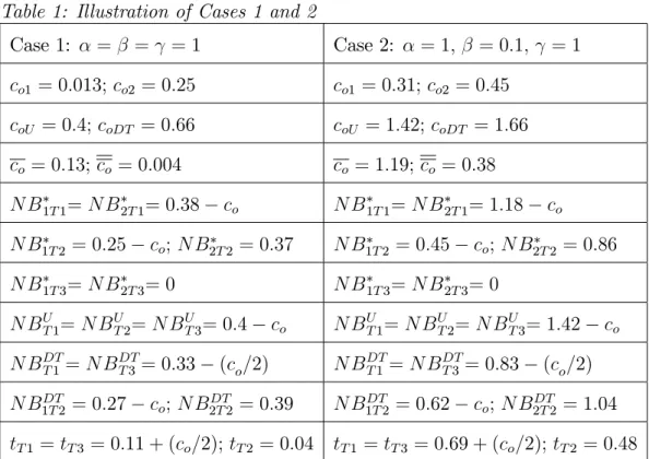
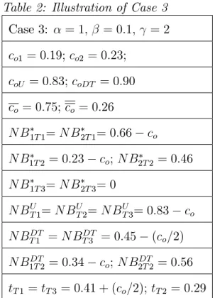
Example: With the above example with quadratic bene…t and
cost functions, we illustrate the three cases of Proposition 5 in Tables 1 and 2 (note that the subscript T j with j = 1; 2; 3 stands for Type 1, Type 2 and Type 3 Nash equilibrium).
Table 1: Illustration of Cases 1 and 2
Case 1: = = = 1 Case 2: = 1; = 0:1; = 1 co1 = 0:013; co2 = 0:25 co1 = 0:31; co2 = 0:45 coU = 0:4; coDT = 0:66 coU = 1:42; coDT = 1:66 co = 0:13; co = 0:004 co = 1:19; co = 0:38 N B1T 1= N B2T 1= 0:38 co N B1T 1= N B2T 1= 1:18 co N B1T 2= 0:25 co; N B2T 2 = 0:37 N B1T 2 = 0:45 co; N B2T 2= 0:86 N B1T 3= N B2T 3= 0 N B1T 3= N B2T 3= 0 N BUT 1= N BUT 2= N BUT 3= 0:4 co N BUT 1= N B U T 2= N B U T 3= 1:42 co N BDTT 1= N BDTT 3= 0:33 (co=2) N BDTT 1= N BDTT 3= 0:83 (co=2) N BDT 1T 2= 0:27 co; N B2T 2DT = 0:39 N B1T 2DT = 0:62 co; N B2T 2DT = 1:04 tT 1= tT 3= 0:11 + (co=2); tT 2= 0:04 tT 1= tT 3= 0:69 + (co=2); tT 2= 0:48
Table 2: Illustration of Case 3 Case 3: = 1; = 0:1; = 2 co1 = 0:19; co2 = 0:23; coU = 0:83; coDT = 0:90 co = 0:75; co = 0:26 N B1T 1= N B2T 1= 0:66 co N B1T 2= 0:23 co; N B2T 2 = 0:46 N B1T 3= N B2T 3= 0 N BUT 1= N BUT 2= N BUT 3= 0:83 co N BDT T 1 = N BT 3DT = 0:45 (co=2) N BDT 1T 2= 0:34 co; N B2T 2DT = 0:56 tT 1= tT 3= 0:41 + (co=2); tT 2= 0:29
Our …ndings as regards Proposition (5.1 and 5.3) can be summarized as follows. The U agreement is preferred by the countries to agreement DT for a su¢ ciently low level of …xed cost of investment. Conversely, when the …xed cost exceeds a threshold level (co > co1 in (1) and co > co in (3)), the
countries are better o¤ under agreement DT. These …ndings illustrate that strictly identical countries can have an interest in reducing their emissions di¤erently, and not in a uniform way. This result can be explained by the assumption of …xed cost in the abatement technology which implies a local non-convexity of the abatement cost function. Identical countries could be better o¤ by signing an agreement based on di¤erentiated standards with transfers in order to take advantage of local increasing returns to scale in
abatement activities. In this case, one of the countries abates for both, and pays for the …xed cost of investment. In return, it is compensated by monetary transfers for this e¤ort. We have shown that in such a case the level of …xed cost must be su¢ ciently high.
A new result emerges for a di¤erent con…guration given by Proposition (5.2). In this case, the preference of countries over the two alternative agree-ments changes as the level of …xed cost increases. The optimality of the U agreement and the DT agreement are occurring by turns. The U agreement which is …rst negotiated for a low level of …xed cost (co < co) could be also
preferred by the countries for a higher level of …xed cost (co2 < co < co).
The DT agreement which is …rst agreed on for a medium level of …xed cost (co < co < co2) could be also negotiated for a high level of …xed cost
(co < co < coDT). The explanation of this result is as follows. As the level
of …xed cost increases, the threat point of negotiations changes. As we have already seen, for each threat point, there exists a threshold level of …xed cost under which it is better to negotiate a U agreement and above which it is better to negotiate a DT agreement. Consequently, as co increases, it
is possible that the type of the best agreement changes because the threat point changes. If we do not observe this alternation (as in cases 1 and 3), it is because for a given threat point, this threshold level of …xed cost (under which it is better to negotiate the U agreement, and above which it is better to negotiate the DT agreement) does not belong to the range of that threat point. In this case, the intuitive result prevails: as co increases from 0, the
best agreement is …rst the U agreement, and above the threshold level of …xed cost, the best agreement is the DT agreement.
The di¤erence in these three con…gurations is due to the forms of the bene…t function B(:) and the variable abatement cost function c(:), which modify the ranking of the threshold levels of …xed cost. In all three con…g-urations, the countries prefer to not cooperate for a very high level of …xed cost (co > coDT). In such a situation, none of the countries abates because it
is too costly (Type 3 Nash equilibrium).
We can now compare the levels of abatement of di¤erent institutional arrangements.
Proposition 6: Given the assumptions on the concavity of the
bene…t function from global abatement B(:) and the convexity of the variable abatement cost function c(:), we have the following ranking of the abatement levels: 2ba > bba and 2a > a1:
Proof. B0(2ba) = c0(ba) < c0(2ba) and B0(bba) = c0(bba): The property that the function B0(:) is decreasing and the function c0(:) is increasing implies that 2ba > bba: A similar argument leads to 2a > a1:
Proposition 6 states that the total abatement is more when both countries make an e¤ort to abate (the case of a uniform standard without transfers) rather than when only one country abates and the other country compensates it for this e¤ort (the case of di¤erentiated standards with transfers). This also holds for the non-cooperative equilibria. To be more speci…c, the level of total
abatement is higher when the two countries abate (Type 1 Nash equilibrium) than when only one of the countries abates (Type 2 Nash equilibrium). This is due to the concavity of the bene…t function and to the convexity of the abatement cost function. Nevertheless, when we take into account the level of individual welfare, which is in‡uenced by the level of …xed cost, we have seen that it could be better that only one of the countries undertakes an abatement e¤ort.
In the next section, we tackle the issue of …xed costs in terms of self-enforcing agreements for numerous countries. The theoretical framework put forward by Barrett (1994) is adopted.
3
Extension: Stability of Agreements
We posit the context of i = 1; 2; :::::N identical countries facing a trans-boundary pollution problem, as is the case when the issue is the climate change or the ozone layer. We will compare the number of countries that join a cooperative agreement for the given two types of agreements: the uni-form (U) and the di¤erentiated (DT) ones. We are guided by the literature on the internal and external stability of IEAs (Barrett (1994), Carraro and Siniscalco (1993)).7 The majority of the models adopting this approach come
7This concept of stability of coalitions is taken from the literature on cartel stability
(d’Aspremont et al. (1983)). This concept has some drawbacks. First, it excludes group deviations. This issue is tackled in Finus and Rundshagen (2003). Secondly, it assumes that a given country believes that other countries do not react to a change in its behaviour. This last point was challenged by the concept of farsighted stability (see for a recent
to the conclusion that the size of the stable coalition is very small, unless pun-ishment strategies in a repeated game framework are taken into account. As de Zeeuw (2008) stresses, trigger mechanisms highlighted in repeated games are similar to the -core concept used in cooperative game theory to analyze the stability of the grand coalition (Chander and Tulkens (1995)).
We assume that the coalition of signatory countries plays Nash equilib-rium strategies with the individual outsiders (non-signatories). The outsiders are also assumed to have Nash equilibrium strategies between them (sym-metric Nash equilibrium). We adopt one of the models in Barrett (1994) with linear bene…t and quadratic cost functions, for which it is possible to obtain
analytical results.8 We also assume that there is a …xed cost in abatement
technology. When a country does not abate, its abatement cost is assumed to be null.
For agreement DT, we posit the existence of an arrangement between (p) signatory countries in the coalition which abate (as > 0) and pay a …xed
cost co; and (m) signatory countries in the coalition which do not abate, but
pay a transfer (t) to other coalition members. Then the number of
non-signatories is N (p + m): Their individual abatement level is represented
by (an): The agreement U is the case with m = 0 and t = 0 : all the
coalition members abate and pay the …xed cost, so there is no need to a
application de Zeeuw (2008)).
8Barrett (1994) assumes that a Stackelberg game is played between the coalition of
signatory countries, which moves …rst, and the outsiders (followers). In the case of a con-stant marginal bene…t function, this assumption yields the same outcomes as those under the assumption of Nash equilibium strategies (Rubio and Casino (2005), p.90, footnote 2).
transfer scheme. The calculations for agreement U are identical to the below calculations of agreement DT by putting m = 0.
Each non-signatory maximizes ex-ante its own utility by taking the abate-ment levels of all other countries as given. The program of a non-signatory is written as follows: max an ( N Bn= w(pas+ i=NP i=p+m+1 ain) co ca2 n 2 ) (3) where w represents the slope of each country’s damage curve and c repre-sents the slope of each country’s marginal abatement cost curve.9 We obtain
ai
n = an =
w
c: We assume that an outsider country will abate if its utility when it abates is higher or equal to that when it does not abate. This con-dition reduces to the following: w p2coc:10 This condition states that the
outsider abates if the marginal bene…t from abatement is su¢ ciently high, or, in other words, if the …xed cost of abatement is su¢ ciently low.
At equilibrium, the utility level of a coalition member which abates and receives a transfer payment (recipient) from other coalition members is
writ-ten in the following way: N Bs = w(pas+(N (m+p))an) co ca
2 s
2 + m
pt:The
9A linear damage function implies that every unit of pollution has a similar marginal
e¤ect on the environment. As Kolstad (2000, p.187) stresses, CO2 emissions could be assumed to exhibit such constant marginal damage. In line with the literature, we assume that returns to scale in abatement technology are diminishing.
10Proof : The utility level of an outsider when it abates is the following:
N Bn1 = w(pas + n=NP n=p+m+1 an) co ca 2 n
2 : Its utility when it does not abate is:
N Bn2= w(pas+ n=NP n=p+m+2
expression of transfers (mp:t) comes from the fact that m countries make a transfer payment t and these total payments are equally shared across p recip-ient countries. At equilibrium, the utility level of a coalition member which does not abate but does make a transfer payment (donor) to other coalition
members, is written in the following way: N Bs= w(pas+(N (m+p))an) t:
We assume that the level of transfers is such that the gains to cooperation are identical across the two groups of signatories.11 This gives us the following
level of transfers: t = p
p + m co+
ca2 s
2 : Subsequently, the utility level of
each coalition member is the following:
N Bs = w(pas+ (N (p + m))an) p p + m co+ ca2 s 2 (4)
As concerns agreement DT, we …rst determine the abatement levels of the p recipient countries in a coalition of (p + m) members. The regulator of the coalition aims to maximize the joint welfare of all its members:
max as (p + m) w(pas+ n=NP n=p+m+1 an) p co+ ca2s 2 (5)
The transfer disappears in the sum. The optimum is achieved for:
as j(p+m)=
(p + m)w
c :
The problem is now to determine (p + m) the number of countries that sign the IEA when the conditions for the internal stability and the external
11For equity reasons, we assume identical transfers for all members. We could also
stability of the coalition are met.
De…nition 2: An IEA consisting of (p + m) signatories must
satisfy the two conditions:
internal stability: N Bn(p + m 1) N Bs(p + m)
external stability: N Bn(p + m) N Bs(p + m + 1)
The internal stability guarantees that a signatory country does not have an incentive to leave the coalition, and the external stability ensures that an outsider country does not have an incentive to join the coalition.
Proposition 7: If non-signatories abate ( w p2coc) :
1) as concerns agreement U ( m = 0), the stable number of countries in the coalition is equal to 2 when the total number of countries is 2, and is equal to 3 when the total number of countries is at least 3:
2) as concerns agreement DT ( m 1), the number of signatories which
abate is 2 ( p = 2) and the number of signatories which make a transfer
pay-ment is any positive number m ( m 1) when the total number of countries
is at least 3. The stable number of countries in the coalition is thus at least 3, providing the possibility for a grand coalition.
Proof: see Appendix.
When the …xed cost of abatement is su¢ ciently low ( w p2coc); our
…ndings as regards Proposition (7.1) replicate the result of Barrett (1994) with linear bene…t and quadratic cost functions. In fact, the agreement
that Barrett (1994) takes into account is identical to the U agreement as it is de…ned in this paper. Here, the existence of a …xed cost in abatement technology is taken into account compared to the model of Barrett (1994). When the …xed cost is su¢ ciently low, as in this case, the countries even abate in the non-cooperative situation. Therefore, they pay the …xed cost both in cooperation and in non-cooperation. We show, as Barrett (1994), that the U agreement is not able to sustain more than two or three signatory countries. In contrast, under the same condition for the level of …xed cost, agreement DT is able to generate a stable coalition if there is precisely two coalition members who abate and pay the …xed cost, with at least one coalition member which …nances their abatement e¤orts. The higher the number of donor countries in the coalition, the larger the size of the stable coalition. It leads that a grand coalition can emerge in the case of a di¤erentiated agreement.
Given the coalition size for each agreement, we now compare the levels of individual payo¤, individual abatement, and global abatement across the U and DT agreements.
Proposition 8: If non-signatories abate ( w p2coc) and if
the total number of countries is at least 3 (N 3) :
1) The individual payo¤ under agreement U (with a coalition size of 3) is higher than that under agreement DT (with a coalition size of 2 + m; with
m 1).
2) The individual abatement under agreement DT is higher or equal to that under agreement U.
3) The global abatement under agreement DT is higher than that under agreement U, if the number of countries which make a transfer payment in agreement DT is at least 5.
Proof: see Appendix.
When the …xed cost of abatement is su¢ ciently low (w p2coc); we
know that the number of countries which abate is 3 for agreement U, and it is equal to 2 for agreement DT. As Proposition (8.2) shows: the higher the number of countries which abate, the lower the level of individual abatement. This leads to the reduction of individual abatement costs in agreement U. This reduction in costs is able to o¤set the lower level of bene…ts from global
abatement, the latter being true for m 5 (Proposition (8.3)). Therefore,
each signatory country is better o¤ under agreement U than under agreement DT (Proposition (8.1)). The global payo¤ associated with an agreement is de…ned as the sum of the payo¤ of signatories and the payo¤ of non-signatories. The comparison of the global payo¤ under agreements U and DT is ambiguous. It depends on the values of the total number of countries,
N, and the number of donor countries in agreement DT, m:
Proposition 9: If non-signatories do not abate ( w <p2coc) :
1) as concerns agreement U ( m = 0), when the total number of countries is at least 2; then the stable number of countries in the coalition is equal to 2 if 2 2coc
w2 , zero if not.
when the total number of countries is 2, then the number of signatories which abate is 1 ( p = 1) and the number of signatories which make a transfer
payment is 1 (m = 1) if 3 2cco
w2 4;
when the total number of countries is at least 3, then the number of sig-natories which abate is 2 ( p = 2) and the number of sigsig-natories which make
a transfer payment must satisfy m + 2 2cco
w2 :
Proof: see Appendix.
When the …xed cost of abatement is su¢ ciently high ( w < p2coc), the
U agreement is not able to sustain more than two signatory countries, no matter the total number of countries a¤ected by the environmental problem. In contrast, under the same condition for the level of …xed cost, agreement DT is able to generate a stable coalition of at least 3 countries, if the total number of countries is su¢ ciently high. Again, the higher the number of donor countries in the coalition, the larger the size of the stable coalition. The high level of …xed costs requires, however, more donor countries in this case. If there was no possibility of transfer payments between countries, the stable coalition would contain only two signatories (this falls into the case of agreement U).
Proposition 10: If non-signatories do not abate ( w < p2coc)
and if the total number of countries is 2 (N = 2) :
1) With a coalition size of 2, the individual payo¤ under agreement U is higher than that under agreement DT.
2) The global payo¤ under agreement U is higher than that under
agree-ment DT if 2 coc
w2.
3) The individual abatement under agreement DT is equal to that under agreement U.
4) The global abatement under agreement U is higher than that under agreement DT.
Proof: see Appendix.
When the …xed cost is su¢ ciently high (w <p2coc)and the total number
of countries is 2, we know that the number of countries which abate is 2 for agreement U, and it is equal to 1 for agreement DT. Proposition (10.3) shows that, under agreement DT, one of the countries makes the abatement equal to the sum of the abatement levels of countries under agreement U. Since the global abatement is higher for agreement U (Proposition (10.4)), this leads to higher bene…ts from global abatement under this agreement. Indeed, this increase in bene…ts under agreement U outperforms the savings in abatement costs allowed by agreement DT. Therefore, individual countries are better o¤ in agreement U (Proposition (10.1)). Remember that the level of …xed cost must be, at the same time, su¢ ciently low in this case, i.e., 2 2coc
w2 ; given by the self-enforcing condition for the U agreement of Proposition 9.1. As concerns global payo¤, it is also higher in agreement U if the level of …xed cost is not too high (Proposition (10.2)).
and if the total number of countries is at least 3 (N 3) :
1) The individual payo¤ under agreement DT (with a coalition size of
2 + m; with m 1) is higher than that under agreement U (with a coalition
size of 2).
2) The global payo¤ under agreement DT is higher than that under
agree-ment U if N 4.
3) The individual abatement under agreement DT is higher than that under agreement U.
4) The global abatement under agreement DT is higher than that under agreement U.
Proof: see Appendix.
When the …xed cost is su¢ ciently high (w <p2coc)and the total number
of countries is at least 3; we know that the number of countries which abate
is 2 for agreement U, and it is equal to 2 + m; with m 1; for agreement
DT. In this case, each country is better o¤ under agreement DT than under agreement U (Proposition (11.1)). The receipt of transfer payments by the two countries in agreement DT provides each of them with the incentive to abate more (Proposition (11.3)), and, in turn, to abate more at the global level (Proposition (11.4)). This leads to higher bene…ts from global abate-ment under agreeabate-ment DT. Furthermore, the DT agreeabate-ment is able to divide the abatement costs across the signatory countries by the means of transfer payments. Remember that the level of …xed cost must be, at the same time, su¢ ciently low in this case, i.e., m + 2 2cco
con-dition for the DT agreement of Proposition 9.2. As concerns global payo¤, it is also higher under agreement DT if the number of signatories is at least 4 (Proposition (11.2)).
To sum up, it would appear that with linear bene…t and quadratic cost functions, agreement U could sustain at most 3 signatory countries. This con…rms Barrett’s (1994) result. Hence, agreement U cannot substantially increase overall payo¤s when the number of countries a¤ected by the envi-ronmental problem is very high. However, agreement DT could lead to a coalition of at least 3 countries. In this case, when the …xed cost is high, the number of donor countries must be su¢ ciently high. By taking into ac-count …xed costs in abatement technology, it would be possible to alter the pessimistic …nding on the small number of signatories of an IEA that is re-ported in the literature. In this case, the agreement must be designed given the di¤erentiated standards with transfers. That is, some of the countries should abate on behalf of all the other countries and pay the …xed cost of abatement. The remaining coalition partners should then compensate them by transfer payments.
4
Conclusion
We investigate the relative e¢ ciency of an agreement based on a uniform standard without transfers and one based on di¤erentiated standards with transfers when strictly identical countries deal with transboundary pollution.
We especially ask what role …xed cost plays. Two approaches are examined: the Nash bargaining solution, implicating two countries, and the coalition formation framework, implicating numerous countries and emphasizing self-enforcing agreements. In the former, in terms of welfare, strictly identical countries may wish to reduce their emissions in a non-uniform way under the di¤erentiated agreement. For this result to hold, the …xed cost of investment in abatement technology must be su¢ ciently high. The nature of the threat point of negotiations, however, also plays a crucial role. As concerns global abatement, the two countries abate more under the uniform agreement than under the di¤erentiated one. In terms of coalition formation when numerous countries are involved, a grand coalition could emerge under a di¤erentiated agreement.
Our results highlight the fact that when the level of …xed cost – arising from the installation of an abatement technology –is accounted for, it could be optimal, even for perfectly symmetric countries, to sign an agreement based on di¤erentiated abatement standards. This analysis could apply to similar and future environmental negotiations, in the case where the cost of the initial investment in abatement activities is too expensive for the coun-tries. This cost could be split between the countries concerned by the en-vironmental problem. This type of enen-vironmental cooperation is already on the European Union agenda in order to strengthen bilateral environmental projects involving southern and eastern Mediterranean countries within the framework of the European Union Neighborhood Policy.
References
[1] d’Aspremont, C., Jacquemin, A., Gabszewicz, J.J., Weymark, J. (1983): On the stability of collusive price leadership, Canadian Jour-nal of Economics, vol. 16, 17-25.
[2] Barrett, S. (1994): Self-enforcing international environmental agree-ments, Oxford Economic Papers, vol.46, 878-894.
[3] Barrett, S. (2003): Environment & Statecraft, The Strategy of Envi-ronmental Treaty-Making, Oxford University Press, New York.
[4] Bayramoglu, B., Jacques, J-F. (2005): Comparison of negotiated uniform vs. di¤erentiated abatement standards for a transboundary pol-lution problem, working paper, Cahiers de recherche EURIsCO [2005.15], Université Paris-Dauphine.
[5] Boyer, M., La¤ont, J-J. (1999): Toward a political theory of the emergence of environmental incentive regulation, Rand Journal of Eco-nomics, vol.30, No.1, 137-157.
[6] Carraro, C., Siniscalco, D. (1993): Strategies for international pro-tection of the environment, Journal of Public Economics, vol. 52, 309-328.
[7] Chander, P., Tulkens, H. (1995): A core-theoretic solution for the design of cooperative agreements on transfrontier pollution, International Tax and Public Finance, vol. 2, 279-294.
[8] Copeland, B., Taylor, S. (2005): Free trade and global warming: a trade theory view of the Kyoto protocol, Journal of Environmental Economics and Management, vol. 49, 205-234.
[9] de Zeeuw, A. (2008): Dynamic e¤ects on the stability of interna-tional environmental agreements, Journal of Environmental Economics and Management, vol. 55, 163-174.
[10] Finus, M., Rundshagen, B. (1998): Toward a positive theory of coali-tion formacoali-tion and endogenous instrumental choice in global pollucoali-tion control, Public Choice, vol. 96, 145-186.
[11] Finus, M. (2001): Game Theory and International Environmental Co-operation, Edwar Elgar, Cheltenman.
[12] Finus, M., Rundshagen, B. (2003): Endogenous coalition formation in global pollution control: a partition function approach, in C.Carraro (ed.), The Endogenous Formation of Economic Coalitions, Edward El-gar, chapter 6, 199-243.
[13] Harstad, B. (2007): Harmonization and side payments in political co-operation, American Economic Review, vol. 97, 871-889.
[14] Hoel, M. (1991): Global environmental problems: the e¤ects of unilat-eral actions taken by one country, Journal of Environmental Economics and Management, vol. 20, 55-70.
[15] Hoel, M. (1992): International environment conventions: the case of uniform reductions of emissions, Environmental and Resource Eco-nomics, vol. 2, 141-159.
[16] Kolstad, C.D. (1987): Uniformity versus di¤erentiation in regulating externalities, Journal of Environmental Economics and Management, vol. 14, 386-399.
[17] Kolstad, C.D. (2000): Environmental Economics, Oxford University Press, New York.
[18] Larson, B.A., Tobey, J.A. (1994): Uncertain climate change and the international policy response, Ecological Economics, vol. 11, 77-84. [19] McAusland, C. (2005): Harmonizing tailpipe policy in symmetric
countries: Improve the environment, improve welfare?, Journal of Envi-ronmental Economics and Management, vol. 50, 229-251.
[20] Nash, J.F. (1950): The bargaining problem, Econometrica, vol. 18, 155-162.
[21] Rubio, S.J., Casino, B. (2005): Self-enforcing international environ-mental agreements with a stock pollutant, Spanish Economic Review, vol. 7, 89-109.
[22] Schelling, T.C. (1960): The Strategy of Con‡ict, Harvard University Press, Cambridge.
[23] Welsch, H. (1992): Equity and e¢ ciency in international CO2
agree-ments, in E.Hope and S.Strom (eds.), Energy Markets and Environmen-tal Issues, Oslo.
APPENDIX
Proof of Lemma 4
The maximization of the function N (a1; a1; t) for agreement U (a1 =
a2 = a and t = 0) leads to the following …rst-order condition: [2B0(2a)
c0(a)][B(2a) c
o c(a) N B2] = [2B0(2a) c0(a)][B(2a) co c(a) N B1].
This condition de…nes a: This holds true for the three Nash equilibria which represent the threat points of the negotiation on agreement U.
The maximization of the function N (a1; a1; t) for agreement DT
(a1 6= 0; a2 = 0 and t 6= 0) leads to the following …rst-order conditions:
(B0(a
1) c0(a1))[B(a1) t N B2] + B0(a1)[B(a1) co c(a1) + t N B1] = 0
and [B(a1) co c(a1) + t N B1] = [B(a1) t N B2].
As concerns Type 1 Nash equilibrium, we have N B1 = N B2 = B(2ba)
co c(ba). Then, the expression of transfers in agreement DT takes the
fol-lowing form, t = (co+c(a1))
2 :Consequently, we obtain (B0(a1) c0(a1))[B(a1) (co+c(a1))
2 B(2ba) + c(ba)] + B0(a1)[B(a1) + co
2
c(a1)
2 B(2ba) + c(ba)] = 0. This
condition leads to a1.
As concerns Type 2 Nash equilibrium, we have N B1 = B(bba) co
c(bba) and NB2 = B(bba). Then, the expression of transfers in agreement DT takes the following form, t = (c(a1) c(bba)
2 : Consequently, we obtain (B0(a1) c0(a1))[B(a1) B(bba) ((c(a1) c(bba)) 2 ] + B0(a1)[B(a1) B(bba) [c(a1) c(bba)] 2 ] = 0.
This condition de…nes a1.
As concerns Type 3 Nash equilibrium, we have N B1 = N B2 = 0. Then,
the expression of transfers in agreement DT is the following, t = [co+c(a1)]
Consequently, we obtain (B0(a
1) c0(a1))[B(a1) (co+c(a2 1))] + B0(a1)[B(a1) (co+c(a1))
2 ] = 0. This condition de…nes a1.
As the expressions of transfers in the three cases show, there exists a unique level of transfers such that the two countries are equally well o¤. This is derived from the de…nition of the Nash bargaining solution and the assumption that all the countries have the same negotiation powers.
Proof of Proposition 2
[B(2a) co c(a)] < h B(a1) [co+c(a2 1)] i if and only if co> co:The (identical) payo¤ of the countries in agreement U when the threat
point is represented by Type 1 Nash equilibrium is the following: [B(2a) co c(a)],
which exceeds their payo¤ at the threat point [B(2ba) co c(ba)] because a
maximizes the function B(2x) co c(x):
Proof of Proposition 3
[B(2a) co c(a)] < B(a1)
[c(a1) c(bba)]
2 if and only if co> co:
The payo¤s of the countries in agreement DT when the threat point is rep-resented by Type 2 Nash equilibrium are the following: B(a1)
[c(a1)+c(bba)]
2 co
for country 1 and B(a1)
[c(a1) c(bba)]
2 for country 2: These payo¤s exceed
those at the threat point (N B1 = B(bba) co c(bba) and NB2 = B(bba)),
because a1 maximizes the function 2B(x) c(x): Consequently, we have
B(a1) c(a21) > B(bba) c(b2ba).
Proof of Proposition 4
[B(2a) co c(a)] < h B(a1) [co+c(a1)] 2 i if and only if co> co:The payo¤ of the countries in agreement U when the threat point is
represented by Type 3 Nash equilibrium is the following: [B(2a) co c(a)] ;
which exceeds 0 if co < coU:
The payo¤ of the countries in agreement DT when the threat point is represented by Type 3 Nash equilibrium is the following: hB(a1) [c(a12)+co]
i ; which exceeds 0 if co < coDT:
Proof of Lemma 5
1) co2 < coU because B(bba) c(bba) < B(2a) c(a). This holds true because
B(2x) > B(x)for every x, since B(:) is an increasing function. Consequently,
the maximum of the function B(2x) c(x)is higher than that of the function
B(x) c(x):
coU < coDT because B(2a) c(a) < 2B(a1) c(a1). This holds true
because B(2x) < 2B(x) by the concavity of the function B(:) and by the assumption that B(0) = 0. Consequently, the maximum of the function
2B(x) c(x) is higher than that of the function B(2x) c(x):
2) We know that co = 2coU coDT, then co < coU because coU < coDT (see
above). Since the inequality coDT > 2coU could exist, co could be negative.
3) co < co because B(2a) c(a) B(a1)
[c(bba) c(a1)]
2 < 2(B(2a) c(a))
(2B(a1) c(a1)) = 2co+ c(bba):
Proof of Proposition 7
We …rst study the condition of internal stability:
N Bn(p + m 1) N Bs(p + m): These utility levels are de…ned in the
N Bn((p 1) + m) = w [(p 1)as+ (N (m + p 1)an] co ca2 n 2 : N Bs(p + m) = w [pas+ (N (m + p))an] p m + p co+ ca2 s 2 : We have as(m + p) = (m + p)w c and an= w c: Substituting, we obtain: N Bn((p 1)+m) = w (p 1) (m + p 1)w c + (N (m + p 1) w c co c 2 w c 2 (6) N Bs(p + m) = w p (m + p)w c + (N (m + p)) w c (7) p m + p " co+ c 2 (m + p)w c 2#
Then, the condition N Bn(p + m 1) N Bs(p + m) reduces to the
following: w2c2 [3 + p(p 4) + m(p 2)] m+pm co:
We now study the condition of external stability:
N Bn(p + m) N Bs(p + m + 1): These utility levels are de…ned in the
following way: N Bn(p + m) = w [(pas+ (N (m + p)an] co ca 2 n 2 : N Bs(p + m + 1) = w [(p + 1)as+ (N (m + p + 1))an] p + 1 m + p + 1 co+ ca2s 2 : We have as(m + p) = (m + p)w c and an= w c: Substituting, we obtain:
N Bn(p + m) = w p (m + p)w c + (N (m + p)) w c co c 2 w c 2 (8) N Bs(p + m + 1) = w (p + 1) (m + p + 1)w c + (N (m + p + 1)) w c(9) p + 1 m + p + 1 " co+ c 2 (m + p + 1)w c 2#
Then, the condition N Bn(p + m) N Bs(p + m + 1) reduces to the
following: 0 < 2cco
w2
m+p+1
m (m(p 1) + p(p 2)):
Let turn now to the core of the proof of Proposition 7.
1) The condition of internal stability is written in the following way in this case (the calculus for agreement U is similar if we put m = 0 and t = 0
in the calculus above): N Bs(p) N Bn(p 1) = w
2 c ( 1 2p 2+ 2p 3 2) 0.
The condition of external stability is (the calculus for agreement U is similar if we put m = 0 and t = 0 in the calculus above): N Bn(p) N Bs(p +
1) = w2 c (
1 2p
2 p) 0:
These conditions are identical to those in Barrett (1994). We will show that only p = 2 and p = 3 satisfy these two conditions.
N Bs(p) N Bn(p 1)is a polynomial in p with a maximum attained for
p = 2. This maximum implies the following value wc2(12) > 0:This polynomial is equal to 0 for p = 1 and p = 3; it is negative for p > 3:
N Bn(p) N Bs(p + 1) is also a polynomial with a minimum attained for
p = 1: This minimum implies the following value wc2( 12) < 0: It is equal to 0 for p = 2 and is strictly positive for p > 2.
2) The condition of internal stability is written in the following way in
this case (see above): (3 + p(p 4) + m(p 2)) m+pm 2cc0
w2 :
The condition of external stability is (see above):
(m(p 1) + p(p 2)) m+p+1m 2cc0
w2 :
For p = 1; we check that the second condition does not hold because
m m+2
2cc0
w2 > 0: For p = 2; these two conditions are written in the following way: the …rst condition 1 m+2m 2cc0
w2 and the second condition m
m m+3 2cc0 w2 ; or 2cCw2 0 1
m+3; which is true for each m strictly positive. We should now
prove that a stable coalition could not exist for p 3 and m 1: Recall
the condition of internal stability (3 + p(p 4) + m(p 2)) m+pm 2cC0
w2 . We
know that (3 + p(p 4) + m(p 2))m+pp exceeds (3 + p(p 4) + m)m+pp when
p 3 and m 1. This latter expression is strictly superior to 1 for p 3
and m 1: However, we have 2cC0
w2 1 by assumption. Consequently, the
condition of internal stability does not hold for p 3 and m 1:
Proof of Proposition 8
1) The individual payo¤ under agreement U (with a coalition size of p = 3) is as follows: N BU
s (3) =
w2(2N +3)
2c co:
The individual payo¤ under agreement DT (with a coalition size of 2 + m;
with m 1) is as follows: N BDT s (2 + m) = w2N c 2co m+2: N BsDT(2 + m) > N BsU(3) if co > 3w2(m+2)
our initial assumption co< w
2
2c: Therefore, N B U
s(3) > N BDTs (2 + m):
2) The individual abatement under agreement DT is: aDT
S (2 + m) =
(2+m)w c :
The individual abatement under agreement U is: aUS(3) = 3wc . We then
have aU
S aDTS because m 1:
3) The global abatement under agreement U is as follows: AU = paU
S + (N m p)an = 33wc + (N 3)wc = wc(6 + N ):
The global abatement under agreement DT is as follows: ADT = paDT
S + (N m p)an= 2(2+m)wc + (N m 2)wc = wc(2 + N + m):
ADT > AU if m 5:
Proof of Proposition 9
We …rst study the condition of internal stability:
N Bn(p + m 1) N Bs(p + m): We have as(m + p) = (m + p)w c and an= 0: We obtain: N Bn(p + m 1) = w (p 1) (m + p 1)w c (10) N Bs(p + m) = w p (m + p)w c p m + p " co+ c 2 (m + p)w c 2# (11)
Then, the condition N Bn(p + m 1) N Bs(p + m) reduces to the
We now study the condition of external stability: N Bn(p + m) N Bs(p + m + 1): We have as(m + p) = (m + p)w c and an = 0: We obtain: N Bn(p + m) = w p (m + p)w c (12) N Bs(p + m + 1) = w (p + 1) (m + p + 1)w c (13) (14) p + 1 m + p + 1 " co+ c 2 (m + p + 1)w c 2#
Then, the condition N Bn(p + m) N Bs(p + m + 1) reduces to the
following: 2ccw2
o(m(1 p) + p(2 p) + 1)
p+1 p+m+1:
Let turn now to the core of the proof of Proposition 9.
1) The condition of internal stability is written in the following way in this case (the calculus for agreement U is similar if we put m = 0 and t = 0
in the calculus above): ( p2+ 4p 2) 2coc
w2 : This inequality does not hold for p = 1 because w2 < 2c
oc: It holds for p = 2 if 2 2cwo2c. Neither it can hold for p = 3 because w <p2coc; nor for p > 3 because 2cwo2c > 0:
We should now prove that the condition of external stability (the cal-culus for agreement U is similar if we put m = 0 and t = 0 in the calcal-culus above) holds for p = 2: In the general case, this condition is written in the
following way ( p2+2p+1) 2coc
w2 , and the case p = 2 satis…es this inequality. 2) The condition of internal stability is written in the following way
(see above): (m(2 p) + p(4 p) 2) m+pp 2cco
w2 .
The condition of external stability is (see above):
(m(1 p) + p(2 p) + 1) m+p+1p+1 2cco
w2 :
For p = 1; the …rst condition leads to (m + 1)2 2cco
w2 ; and the second
condition implies (m + 2) 2cC0
w2 . Since the total number of countries is 2; the number of signatories which make a transfer is 1 (m = 1). Consequently, the two conditions imply the following relationship 3 2cco
w2 4.
For p > 2 and m 1; we note that the condition of internal stability
(m(2 p) + p(4 p) 2)is lower than (2 p) + p(4 p) 2 = p2+ 3p. This
…nal expression is a polynomial with an integer maximum attained for p = 1 and p = 2. These maxima imply the following value (2). This polynomial is inferior or equal to zero for p 3:Consequently, the condition of internal
stability does not hold for p 3:
For p = 2; the condition of internal stability is equal to 2 m+22 2cco
w2 :This holds for a given value of m higher than a threshold level, if the total number of countries is su¢ ciently high. The condition of external stability is equal
to (1 m) m+33 2cco
w2 ; which always holds for m 1:
Proof of Proposition 10
1) The individual payo¤ under agreement U (with a coalition size of p = 2) is as follows: N BU
s (2) = 2w2
c co:
as follows: N BDT s (2) = w2 c co 2: N BDT
s (2) > N BsU(2) if w2 < cc2o;which is incompatible with the
assump-tion co w
2
c needed to have a coalition size of 2 in agreement U. Therefore,
N BUs(2) > N BsDT(2):
2) The global payo¤ under agreement U (with a coalition size of p = 2) is as follows: VU(2) = (m + p)N BU s + (N m p)N BnU = 2 h 2w2 c co i = 4wc2 2co;
because there is no non-signatory for N = 2:
The global payo¤ under agreement DT (with a coalition size of m+p = 2) is as follows: VDT(2) = (m + p)N BsDT + (N m p)N BnDT = 2hwc2 co 2 i = 2w2 c co: VU(2) > VDT(2) if w >pcco 2 :
3) The individual abatements under agreements U and DT are as follows: aU
S(2) = aDTS (2) = 2w
c .
4) The global abatement under agreement U is as follows: AU = 2aU S(2) = 4w
c :
The global abatement under agreement DT is as follows: ADT = aDTS (2) =
2w c :
We have ADT < AU:
Proof of Proposition 11
1) The individual payo¤ under agreement U (with a coalition size of p = 2) is as follows: N BU
s (2) = 2w2
c co: