Residual Networks for Computer Go

IEEE TCIAIG 1

Residual Networks for Computer Go

Tristan Cazenave

Universit´e Paris-Dauphine, PSL Research University, CNRS, LAMSADE, 75016 PARIS, FRANCE

Deep Learning for the game of Go recently had a tremendous success with the victory of AlphaGo against Lee Sedol in March 2016. We propose to use residual networks so as to improve the training of a policy network for computer Go. Training is faster than with usual convolutional networks and residual networks achieve high accuracy on our test set and a 4 dan level.

Index Terms—Deep Learning, Computer Go, Residual Networks.

I. INTRODUCTION

D

EEP Learning for the game of Go with convolutional neural networks has been addressed by Clark and Storkey [1]. It has been further improved by using larger networks [2]. Learning multiple moves in a row instead of only one move has also been shown to improve the playing strength of Go playing programs that choose moves according to a deep neural network [3]. Then came AlphaGo [4] that combines Monte Carlo Tree Search (MCTS) with a policy and a value network.

Deep neural networks are good at recognizing shapes in the game of Go. However they have weaknesses at tactical search such as ladders and life and death. The way it is handled in AlphaGo is to give as input to the network the results of ladders. Reading ladders is not enough to understand more complex problems that require search. So AlphaGo combines deep networks with MCTS [5]. It learns a value network from self-played games in order to evaluate positions. When playing, it combines the evaluation of a leaf of the Monte Carlo tree by the value network with the result of the playout that starts at this leaf. The value network is an important innovation due to AlphaGo. It made a large improvement in the level of play.

One of the problems about training a value network is that millions of games have to be played by the policy network against different versions of itself in order to create the data used to train the value network. It is therefore interesting to find a way to learn with less training examples so as to reduce the bottleneck of playing millions of games. Learning with less examples also often implies that in the end the accuracy of the network on the training set is greater.

Residual Networks improve the training of very deep net-works [6]. These netnet-works can gain accuracy from consider-ably increased depth. On the ImageNet dataset a 152 layers networks achieves 3.57% error. It won the 1st place on the ILSVRC 2015 classification task. The principle of residual nets is to add the input of the layer to the output of each layer. With this simple modification training is faster and enables deeper networks. We propose to use residual networks for computer Go in order to train networks faster, to increase accuracy and also to enable training deeper networks.

The second section details the use of residual networks for computer Go, the third section gives experimental results, and

ReLU

Output Convolution

Input

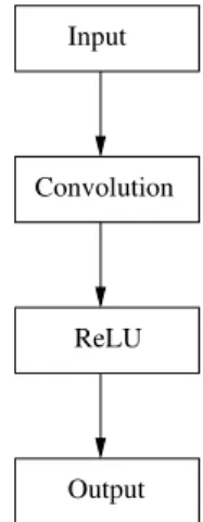
Fig. 1. The usual layer for computer Go.

the last section concludes.

II. RESIDUALLAYERS

The usual layer used in computer Go program such as Al-phaGo [2] and DarkForest [3] is composed of a convolutional layer and of a ReLU layer as shown in figure 1.

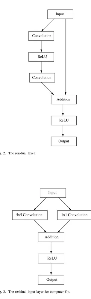
The residual layer used for image classification adds the input of the layer to the output of the layer. It uses two convolutional layers before the addition. The ReLU layers are put after the first convolutional layer and after the addition. The residual layer is shown in figure 2. We will experiment with this kind of residual layers for our Go networks.

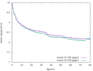
The input layer of our Go networks is also residual. It uses a 5 × 5 convolutional layer in parallel to a 1 × 1 convolutional layer and adds the outputs of the two layers before the ReLU layer. It is depicted in figure 3.

The output layer of the network is a 3 × 3 convolutional layer with one output plane followed by a SoftMax. All the hidden layers use 256 feature planes and 3 × 3 filters.

We define the number of layers of a network as the number of convolutional layers. So a 28 layers network has 28 convolutional layers corresponding to 14 layers depicted in figure 2.

III. EXPERIMENTALRESULTS

In this section we will explain how we conducted the exper-iments evaluating deep residual networks. We first present the

IEEE TCIAIG 2 Input Convolution ReLU Convolution Addition ReLU Output

Fig. 2. The residual layer.

Input

Addition

ReLU

Output

5x5 Convolution 1x1 Convolution

Fig. 3. The residual input layer for computer Go.

data that was used for training and testing. We then describe the input and output planes of the networks and the training and testing phases with results given as percentages on the test set. We finish the section describing our Go playing program Golois. All experiments were done using Torch [7].

A. The Data

Our training set consists of games played between 2000 and 2014 on the Kiseido Go Server (KGS) by players being 6 dan or more. We exclude handicap games.

Each position can be rotated and mirrored to its eight possible symmetric positions. It results in approximately 160 000 000 positions in the training set.

The test set contains the games played in 2015. The posi-tions in the test set are not mirrored and there are 500 000 different positions in the test set.

The dataset is similar to the AlphaGo and the DarkForest datasets, all the games we have used for training are part of these two other datasets. AlphaGo also uses games by weaker players in its dataset [2], instead we only use games by 6 dan or more, it probably makes the dataset more difficult and more meaningful. The AlphaGo dataset is not available, also it would help to have the 30 000 000 games played by AlphaGo against itself so as to train a value network but this dataset is not available either.

We also used the GoGoD dataset. It is composed of many professional games played until today. We used the games from 1900 to 2014 for the training set and the games from 2015 and 2016 as the test set. In our experiments we use the first 500 000 positions of the test set to evaluate the error and the accuracy of the networks.

B. Input and Output Planes

The networks use 45 19 × 19 input planes: three planes for the colors of the intersections, one plane filled with ones, one plane filled with zeros, one plane for the third line, one plane filled with one if there is a ko, one plane with a one for the ko move, ten planes for the liberties of the friend and of the enemy colors (1, 2, 3, 4, ≥ 5 liberties), fourteen planes for the liberties of the friend and of the enemy colors if a move of the color is played on the intersection (0, 1, 2, 3, 4, 5, ≥ 6 liberties), one plane to tell if a friend move on the intersection is captured in a ladder, one plane to tell if a string can be captured in a ladder, one plane to tell if a string is captured in a ladder, one plane to tell if an opponent move is captured in a ladder, one plane to tell if a friend move captures in a ladder, one plane to tell if friend move escapes a ladder, one plane to tell if a friend move threatens a ladder, one plane to tell is an opponent move threatens a ladder, and five planes for each of the last five moves.

The output of a network is a 19 × 19 plane and the target is also a 19 × 19 plane with a one for the move played and zeros elsewhere.

C. Training

In order to train the network we build minibatches of size 50 composed of 50 states chosen randomly in the training set,

IEEE TCIAIG 3

each state is randomly mirrored to one of its eight symmetric states. The accuracy and the error on the test set are computed every 5 000 000 training examples. We define an epoch as 5 000 000 training examples.

The updating of the learning rate is performed using algo-rithm 1. A step corresponds to 5 000 training examples. Every 1000 steps the algorithm computes the average error over the last 1000 steps and the average error over the step minus 2000 to the step minus 1000. If the average error increases then the learning rate is divided by 2. The initial learning rate is set to 0.2. The algorithm stays at least 4000 steps with the same learning rate before dividing it by 2.

Algorithm 1 The algorithm used to update the training rate. if nbExamples % 5000 == 0 then

step ← step + 1

if step % 1000 == 0 then error1000 ←P

last 1000 steps(errorStep)

error2000 ←P

step − 2000 to step − 1000(errorStep)

if step - lastDecrease > 3000 then if error2000 < error1000 then

rate ← rate₂ lastDecrease ← step end if end if end if end if

The evolution of the accuracy on the KGS test set is given in figure 4. The horizontal axis gives the number of epochs. The 20 layers residual network scores 58.2456%. We also give the evolution of the accuracy of a 13 layers vanilla network of the same type as the one described in the AlphaGo papers. We can see that the accuracy of the smaller non residual network is consistently smaller.

In order to further enhance accuracy we used bagging. The input board is mirrored to its 8 possible symmetries and the same 20 layers network is run on all 8 boards. The outputs of the 8 networks are then mirrored back and summed. Bagging improves the accuracy up to 58.5450%. The use of symmetries is similar to AlphaGo.

In comparison, AlphaGo policy network with bagging reaches 57.0% on a similar KGS test set and Darkforest policy network reaches 57.3%.

The evolution of the mean square error on the test set is given in figure 5. We can observe that the error of the 20 layers residual network is consistently smaller than the one of the non residual 13 layers network.

Figures 6 and 7 give the accuracy and the error on the GoGoD test set for 20 residual layers and 28 residual layers networks. Going from 20 layers to 28 layers is a small improvement.

In order to test the 28 layers residual networks we organized a round robin tournament between 10 of the last networks, going from epoch 70 to epoch 79 of the training. The results are given in table I. The network that has the best raw accuracy on the GoGoD test set is the network of epoch 71 with 54.6042% accuracy. When improved with bagging it reaches

Fig. 4. Evolution of the accuracy on the KGS test set.

Fig. 5. Evolution of the error on the KGS test set.

IEEE TCIAIG 4

Fig. 7. Evolution of the error on the GoGoD test set. TABLE I

ROUND ROBIN TOURNAMENT BETWEEN28LAYERSGOGODNETWORKS. Epoch Test error Test accuracy Games won Score 70 8.1108971917629 54.5606 256/540 0.474074 71 8.1061121976376 54.6042 282/540 0.522222 72 8.1098112225533 54.3868 286/540 0.529630 73 8.0968823492527 54.4516 271/540 0.501852 74 8.1007176065445 54.4184 268/540 0.496296 75 8.1010078394413 54.4528 247/540 0.457407 76 8.0951432073116 54.4934 271/540 0.501852 77 8.1806340968609 54.0784 284/540 0.525926 78 8.1806341207027 54.0784 294/540 0.544444 79 8.1806340968609 54.0784 241/540 0.446296

54.9954% on the GoGoD test set. However the network that has the best score is the network of epoch 78 which has a score against the other networks of 0.544444 which is better than the network of epoch 71 that has a score of 0.522222. The epoch 78 network has a 55.0306% accuracy when combined with bagging.

D. Golois

We made the 20 layers residual network with bagging and a 58.5450% accuracy play games on the KGS internet Go server. The program name is Golois4 and it is quite popular, playing 24 hours a day against various opponents. It is ranked 3 dan.

Playing on KGS is not easy for bots. Some players take advantage of the bot behaviors such as being deterministic, so we randomized play choosing randomly among moves that are evaluated greater than the evaluation of the best move when augmented by 0.05. Golois4 plays its moves almost instantly thanks to its use of a K40 GPU. It gives five periods of 15 seconds per move to its human opponents.

We also made the best residual network with 28 layers play on KGS under the name Golois6 and it reached 4 dan.

In comparison, AlphaGo policy network and DarkForest policy network reached a 3 dan level using either reinforce-ment learning [4] or multiple output planes giving the next moves to learn and 512 feature planes [3].

IV. CONCLUSION

The usual architecture of neural networks used in computer Go can be much improved. Using residual networks helps training the network faster and training deeper networks. A residual network with 20 layers scores 58.2456% on the KGS test set. It is greater than previously reported accuracy. Using bagging of mirrored inputs it even reaches 58.5450%. The 20 layers residual network with bagging plays online on KGS and reached a 3 dan level playing almost instantly. The 28 layers residual network trained on the GoGoD dataset reached 4 dan. For future work we intend to use residual networks to train a value network. We could also perform experiments as in [8].

ACKNOWLEDGMENT

The author would like to thank Nvidia and Philippe Van-dermersch for providing a K40 GPU that was used in some experiments.

REFERENCES

[1] C. Clark and A. Storkey, “Training deep convolutional neural networks to play go,” in Proceedings of the 32nd International Conference on Machine Learning (ICML-15), 2015, pp. 1766–1774.

[2] C. J. Maddison, A. Huang, I. Sutskever, and D. Silver, “Move evalu-ation in go using deep convolutional neural networks,” arXiv preprint arXiv:1412.6564, 2014.

[3] Y. Tian and Y. Zhu, “Better computer go player with neural network and long-term prediction,” arXiv preprint arXiv:1511.06410, 2015. [4] D. Silver, A. Huang, C. J. Maddison, A. Guez, L. Sifre, G. van den

Driessche, J. Schrittwieser, I. Antonoglou, V. Panneershelvam, M. Lanc-tot, S. Dieleman, D. Grewe, J. Nham, N. Kalchbrenner, I. Sutskever, T. Lillicrap, M. Leach, K. Kavukcuoglu, T. Graepel, and D. Hassabis, “Mastering the game of go with deep neural networks and tree search,” Nature, vol. 529, no. 7587, pp. 484–489, 2016.

[5] R. Coulom, “Efficient selectivity and backup operators in Monte-Carlo tree search,” in Computers and Games, 5th International Conference, CG 2006, Turin, Italy, May 29-31, 2006. Revised Papers, ser. Lecture Notes in Computer Science, H. J. van den Herik, P. Ciancarini, and H. H. L. M. Donkers, Eds., vol. 4630. Springer, 2006, pp. 72–83.

[6] K. He, X. Zhang, S. Ren, and J. Sun, “Deep residual learning for image recognition,” in 2016 IEEE Conference on Computer Vision and Pattern Recognition, CVPR 2016, Las Vegas, NV, USA, June 27-30, 2016, 2016, pp. 770–778. [Online]. Available: http://dx.doi.org/10.1109/CVPR.2016.90

[7] R. Collobert, K. Kavukcuoglu, and C. Farabet, “Torch7: A matlab-like environment for machine learning,” in BigLearn, NIPS Workshop, no. EPFL-CONF-192376, 2011.

[8] A. Veit, M. J. Wilber, and S. J. Belongie, “Residual networks behave like ensembles of relatively shallow networks,” in Advances in Neural Information Processing Systems 29: Annual Conference on Neural Information Processing Systems 2016, December 5-10, 2016, Barcelona, Spain, 2016, pp. 550–558. [Online]. Available: http://papers.nips.cc/paper/ 6556-residual-networks-behave-like-ensembles-of-relatively-shallow-networks

Tristan Cazenave Professor of Artificial Intelli-gence at LAMSADE, University Paris-Dauphine, PSL Research University. Author of more than a hundred scientific papers about Artificial Intelli-gence in games. He started publishing commercial video games at the age of 16 and defended a PhD thesis on machine learning for computer Go in 1996 at University Paris 6.