Generalized k-means based clustering for temporal data under time warp

(1)

HAL Id: tel-01394280

https://hal.archives-ouvertes.fr/tel-01394280v2

Submitted on 13 Nov 2017

HAL is a multi-disciplinary open access

archive for the deposit and dissemination of sci-entific research documents, whether they are pub-lished or not. The documents may come from teaching and research institutions in France or abroad, or from public or private research centers.

L’archive ouverte pluridisciplinaire HAL, est destinée au dépôt et à la diffusion de documents scientifiques de niveau recherche, publiés ou non, émanant des établissements d’enseignement et de recherche français ou étrangers, des laboratoires publics ou privés.

under time warp

Saeid Soheily-Khah

To cite this version:

Saeid Soheily-Khah. Generalized k-means based clustering for temporal data under time warp. Arti-ficial Intelligence [cs.AI]. Universite Grenoble Alpes, 2016. English. �tel-01394280v2�

(2)

THÈSE

pour obtenir le grade de

DOCTEUR DE L’UNIVERSITÉ DE GRENOBLE

Spécialité : Informatique et Mathématiques appliquées Arrêté ministériel : 7 août 2006

Présentée par

Saeid SOHEILY-KHAH

Thèse dirigée par Ahlame DOUZAL et codirigée par Eric GAUSSIER

préparée au sein du

Laboratoire d’Informatique de Grenoble (LIG) dans l’école doctorale Mathématiques, Sciences et Technologies de l’Information, Informatique (MSTII)

Generalized k-means based clustering

for temporal data under time warp

Thèse soutenue publiquement le 7 OCT 2016,

devant le jury composé de: Mohamed NADIF

Professeur, LIPADE, University of Paris Descartes, Rapporteur Paul HONEINE

Professeur, LITIS, Université de Rouen Normandie, Rapporteur Pierre-François MARTEAU

Professeur, IRISA, Université Bretagne Sud, Examinateur, Présidente du jury

Jose Antonio VILAR FERNANDEZ

Maître de conférences, MODES, Universidade da Coruña, Examinateur

Ahlame DOUZAL

Maître de conférences (HDR), LIG, Université Grenoble Alpes, Directeur de thèse

Eric GAUSSIER

(3)

(4)

UNIVERSITÉ DE GRENOBLE

ÉCOLE DOCTORALE MSTII

Description de complète de l’école doctorale

T H È S E

pour obtenir le titre de

docteur en sciences

de l’Université de Grenoble-Alpes

Mention : Informatique et Mathématiques appliquées

Présentée et soutenue par

Saeid SOHEILY-KHAH

Generalized k-means based Clustering

for Temporal Data under Time Warp

Thèse dirigée par Ahlame DOUZAL et

codirigée par Eric GAUSSIER

préparée au Laboratoire d’Informatique de Grenoble (LIG)

soutenue le 7 OCT 2016

Jury :

Rapporteurs : Mohamed NADIF - LIPADE, University of Paris Descartes

Paul HONEINE - LITIS, Université de Rouen Normandie

Directeur : Ahlame DOUZAL - LIG, Université Grenoble Alpes

Co-Directeur : Eric GAUSSIER - LIG, Université Grenoble Alpes

Président : Pierre-François MARTEAU - IRISA, Université Bretagne Sud

Examinateur : Jose Antonio VILAR FERNANDEZ - MODES, Universidade da Coruña

(5)

(6)

Acknowledgments

First and foremost, I would like to express my gratitude to my dear adviser, Ahlame DOUZAL, for her support, patience, and encouragement throughout my graduate studies. It has been an honor to be her Ph.D. student. It is not often that one finds an adviser and colleague that always finds the time for listening to the little problems and roadblocks that unavoidably crop up in the course of performing research. Her technical and editorial advice was essential to the completion of this dissertation and has taught me innumerable lessons and insights on the workings of academic research in general. She has been great teacher who has prepared me to get to this place in my academic life.

I have been extremely lucky to have a co-supervisor, Eric GAUSSIER, who cared about my work, and who responded to my questions and queries so promptly. I appreciate his wide knowledge and his assistance in writing reports (i.e., conference papers, journals and this thesis). He provided me with direction, technical support and became more of a mentor and friend, than a professor.

I would like to thank my dissertation committee members Mohamed NADIF, Paul HONEINE, Pierre-François MARTEAU and Jose Antonio VILAR FERNANDEZ for their interest in my work. They have each provided helpful feedback.

Completing this work would have been all the more diﬃcult were it not for the support and friendship provided by the other members of the AMA team in Laboratoire d’Informatique de Grenoble. I am indebted to them for their help.

I want to thank my parents, who brought a 80-86 computer into the house when I was still impressionable enough to get sucked into a life of computer science. My parents, Ali and Safa, receive my deepest gratitude and love for their dedication and the many years of support during my undergraduate studies that provided the foundation for this work. I doubt that I will ever be able to convey my appreciation fully, but I owe them my eternal gratitude.

Last, but not least, I would like to thank my wife, Zohreh, for standing beside me through-out my career and writing this thesis, and also for her understanding and love during the past few years. She has been my inspiration and motivation for continuing to improve my knowl-edge and move my career forward. Her support and encouragement was in the end what made this dissertation possible. She is my rock, and I dedicate this thesis to her.

(7)

(8)

List of Figures

1.1 Three possible alignments (paths) between xi and xj . . . 12

1.2 dynamic time warping alignment (left) vs. euclidean alignment (right) . . . 12 1.3 The optimal alignment path between two sample time series with time warp (left),

without time warp (right) . . . 13 1.4 Speed up DTW using constraints: (a)Sakoe-Chiba band (b)Asymmetric Sakoe-Chiba

band (c)Itakura parallelogram . . . 14 1.5 The constrained optimal alignment path between two sample time series (Sakoe-Chiba

band = 5 - left), (Itakura parallelogram - right) . . . 15 1.6 The time series sequence xi, and its PAA x∗i . . . 16

1.7 Alignment between two time series by (a)DTW (b)PDTW . . . 16 1.8 (a) The optimal alignment warp path on level 2. (b) The optimal alignment warp path

with respect to the constraint region R by projecting alignment path to level 1. (c) The optimal alignment warp path with δ = 2 . . . 17 1.9 Example of comparison of COR vs CORT (r = 1). COR(x1, x2) = – 0.90, COR(x1, x3)

= – 0.65, COR(x2, x3) = 0.87, CORT(x1, x2) = – 0.86, CORT(x1, x3) = – 0.71,

CORT(x2, x3) = 0.93. . . 19

1.10 Comparison of time series: similar in value, opposite in behavior (left), similar in behavior (right) . . . 20 1.11 Kernel trick: embed data into high dimension space (feature space) . . . 21 2.1 Pairwise temporal warping alignment between x and y (left), the estimation of the

centroid c of time series x and time series y in the embedding Euclidean space (right). A dimension i in the embedded Euclidean space identifies a pairwise link ai. . . 30

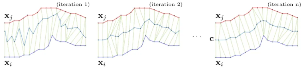
2.2 Three possible alignments (paths) are displayed between xiand xj, π∗(the green one)

being the dynamic time warping one. The centroid c(xi, xj) = (c1, ..., c8) is defined as

the average of the linked elements through π∗_{, with for instance c}

3= Avg(xi2, xj3).. . 31

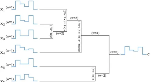
2.3 Medoid as a prototype . . . 32 2.4 Centroid estimation by random pairwise centroid combination. . . 33 2.5 Centroid estimation by centroid combination through clustering dendrogram. . . 34

(11)

2.6 Example of six time series sequence averaging using PSA . . . 35

2.7 Centroid estimation based on a reference time series. The DTW is performed between time series x1, x2 and the reference time series x3 (left). Time series x1 and x2 are embedded in the space defined by x3 (right) where the global centroid is estimated, and ’avg’ is the standard mean function. . . 36

2.8 DBA iteratively adjusting the average of two time series xi and xj . . . 36

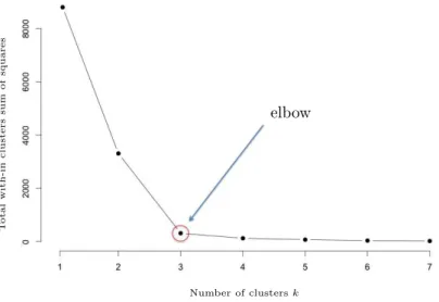
3.1 The elbow method suggests k=3 cluster solutions . . . 41

3.2 k-means: diﬀerent initializations lead to diﬀerent clustering results . . . 43

3.3 Outliers eﬀect: k-means clustering (left) vs. k-medoids clustering (right) . . . 44

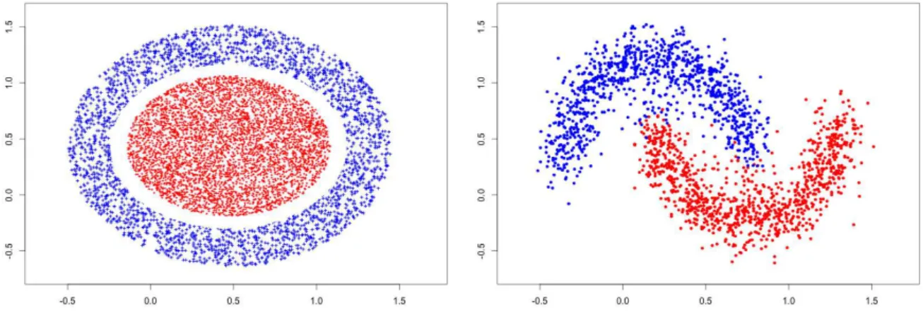
3.4 Non-linearly separable clusters . . . 45

3.5 The kernel trick - complex in low dimension (left), simple in higher dimension (right) 45 3.6 k-means clustering (left) vs. kernel k-means clustering (right) . . . 46

3.7 Three possible alignments are displayed between x = (x1, ..., x7) and c = (c1, ..., c7) and w = (w1, ..., w7) in the 7× 7 grid. The value of each cell is the weighted divergence f (wt) ϕt′t = f (wt) ϕ(xit′, ct) between the aligned elements xt′ and ct. The optimal path π∗ (the green one) that minimizes the average weighted divergence is given by π1= (1, 2, 2, 3, 4, 5, 6, 7) and π2= (1, 2, 3, 4, 4, 5, 6, 7).. . . 51

4.1 The time series behaviors within the classes "Funnel", "Cyclic" and "Gun" of the datasets cbf, cc and gunpoint, respectively. . . 66

4.2 The time series behaviors within the classes "Begin", "Down" and "Warm" of the datasets bme, umd and consseason, respectively.. . . 66

4.3 Structures underlying datasets . . . 67

4.4 The time series behaviors within the three classes of dataset bme . . . 70

4.5 The time series behaviors within the three classes of dataset umd . . . 70

4.6 CC clusters based on κDTAK dissimilarities . . . 72

4.7 Global comparison of the clustering Rand index . . . 73

4.8 Global comparison of the clustering Time consumption . . . 74

4.9 Global comparison of the nearest centroid classification error rate (k=1) . . . . 79

(12)

List of Figures vii

4.11 Latent curve z and three induced instances x1, x2, x3 without noise (left), and with

noise ei (right) - spiral dataset . . . 83

4.12 Latent curve z and three induced instances x1, x2, x3 sharing local characteristics for

the spiral2dataset . . . 84 4.13 spiral₂_{: Progression of the 2-D spatial coordinates (x, y) and the noise dimension e}

over time for the spiral2dataset . . . 84

4.14 cbf_{-"Funnel" centroids: (a) Initial time series, (b) NLAAF, (c) PSA, (d) CWRT, (e)} DBA, (f) WDTW, (g) WKDTAK, (h) WKGDTW . . . 85

4.15 cc_{-"Cyclic" centroids: (a) Initial time series, (b) NLAAF, (c) PSA, (d) CWRT, (e)} DBA, (f) WDTW, (g) WKDTAK, (h) WKGDTW . . . 85

4.16 umd_{-"Down" centroids: (a) Initial time series, (b) NLAAF, (c) PSA, (d) CWRT, (e)} DBA, (f) WDTW, (g) WKDTAK, (h) WKGDTW . . . 86

4.17 spiral_{centroids: (a) Initial time series, (b) NLAAF, (c) PSA, (d) CWRT, (e) DBA,} (f) WDTW, (g) WKDTAK, (h) WKGDTW . . . 86

4.18 spiral2_{centroids: (a) Initial time series, (b) NLAAF, (c) PSA, (d) CWRT, (e) DBA,} (f) WDTW, (g) WKDTAK, (h) WKGDTW . . . 87

4.19 spiral2-x _{centroids: (a) Initial time series, (b) NLAAF, (c) PSA, (d) CWRT, (e)} DBA, (f) WDTW, (g) WKDTAK, (h) WKGDTW . . . 87

4.20 spiral2-x _{centroids: centroid (left) and weight (right) estimation through the first} iterations of WDTW . . . 88 4.21 spiral2-x _{centroids: centroid (left) and weight (right) estimation through the first}

iterations of WKDTAK . . . 89

4.22 Comparison of average Rand index values . . . 90 4.23 Three samples classes of character trajectories-"e", "o" and "p": the ground

(13)

(14)

List of Tables

1.1 Kernel function examples . . . 23

3.1 Comparison between k-means and k-medoids . . . 44

4.1 Data description . . . 68

4.2 Parameter Line / Grid: The⊙ multiplication operator is element-wise (e.g. {1, 2, 3} ⊙ med= {med, 2med, 3med}). med(x) stands for the empirical median of x evaluated on the validation set and x and y are vectors sampled randomly within time series in the validation set. . . 69

4.3 Clustering Rand index . . . 71

4.4 Clustering time consumption(sec.) . . . 75

4.5 Classification error rate (k=1) . . . 78

4.6 Nearest centroid classification error rate (k=1). . . 79

4.7 Classification time consumption (k=1) . . . 81

4.8 Classification average ranking (k=1) . . . 82

4.9 p-value (X2_{-test: uniformity distribution test)} _{. . . 91}

(15)

(16)

Table of Acronyms

LIG _{Laboratoire d’Informatique de Grenoble} AMA _{Apprentissage, Méthode et Algorithme}

DTW _{Dynamic Time Warping}

NLAAF _{NonLinear Alignment and Averaging Filters} PSA _{Prioritized Shape Averaging}

CWRT _{Cross-Words Reference Template} DBA _{Dtw Barycebter Averaging} SDTW _{Scaled Dynamic Time Warping} COR _{Pearson CORrelation coeﬃcient} CORT _{Temporal CORrelation coeﬃcient}

DACO _{Diﬀerence between Auto-Correlation Operators} PAA _{Piecewise Aggregate Approximation}

PDTW _{Piecewise Dynamic Time Warping} DTW_sc _{Sakoe-Chiba Dynamic Time Warping} DTAK _{Dynamic Time Alignment Kernel} PAM _{Partitioning Around Medoids} CLARA _{Clustering LARge Applications} MDS _{Multi Dimensional Scaling}

MCA _{Multiple Correspondence Analysis}

CA _{Correspondence Analysis}

RBF _{Radial Basis Function}

K_CORT _{Temporal Correlation Coeﬃcient Kernel} K_DACO _{Auto-correlation Kernel}

K_{DT W} _{Dynamic Time Warping Kernel}

K_SC _{Sakoe-Chiba Dynamic Time Warping Kernel} xi

(17)

K_{GDT W} _{Gaussian Dynamic Time Warping Kernel} K_{GDT W}

SC Sakoe-Chiba Gaussian Dynamic Time Warping Kernel

K_{DT AK} _{Dynamic Temporal Alignment Kernel} K_{DT AK}

SC Sakoe-Chiba Dynamic Temporal Alignment Kernel

K_GA _{Global Alignment Kernel}

K_{T GA} _{Triangular Global Alignment Kernel} WDTW _{Weighted Dynamic Time Warping}

WK_{GDT W} _{Weighted Gaussian Dynamic Time Warping Kernel} WK_{DT AK} _{Weighted Dynamic Temporal Alignment Kernel} WK_GA _{Weighted Global Alignment Kernel}

(18)

Introduction

Due to rapid increase in data size, the idea of discovering hidden information in datasets has been exploded extensively in the last decade. This discovery has been centralized mainly on data mining, classification and clustering. One major problem that arises during the mining process is handling data with temporal feature. Temporal data naturally arise in various emerging applications as sensor networks, dynamic social networks, human mobility or internet of things. Temporal data refers to data, where changes over time or temporal aspects play a central role or are of interest. Unlike static data, there is high dependency among time series or sequences and the appropriate treatment of data dependency or correlation becomes critical in any temporal data processing.

Temporal data mining has recently attracted great attention in the data mining community [BF98]; [HBV01]; [KGP01]; [KLT03]. Basically temporal data mining is concerned with the analysis of temporal data and for finding temporal patterns and regularities in sets of temporal data. Since temporal data mining brings together techniques from different fields such as statistics, machine learning and databases, the literature is diffused among many different sources. According to the techniques of data mining and theory of statistical time series analysis, the theory of temporal data mining may involve the following areas of investigation since a general theory for this purpose is yet to be developed [LOW02]. Temporal data mining tasks include: characterization and representation, similarity computation and comparison, temporal association rules, clustering, classification, prediction and trend analysis, temporal pattern discovery, etc.

Clustering temporal data is a fundamental and important task, usually applied prior to any temporal data analysis or machine learning tasks, for summarization, extraction groups of time series and highlight the main underlying dynamics; all the more crucial for dimensionality reduction in big data context. Clustering problem is about partitioning a given dataset into groups or clusters such that the data points in a cluster are more similar to each other than data points in different clusters [GRS98]. It may be found under different names in different contexts, such as "unsupervised learning" in pattern recognition, "numerical taxonomy" in biology, "typology" in social sciences and "partition" in graph theory [TK99]. There are many applications where a temporal data clustering activity is relevant. For example in web activity logs, clusters can indicate navigation patterns of different user groups. In financial data, it would be of interest to group stocks that exhibit similar trends in price movements. Another example could be clustering of biological sequences like proteins or nucleic acids, so that sequences within a group have similar functional properties [F.88]; [Mil+99]; [Osa+02]. Hense, there are a variety of methods for clustering of temporal data and many of usual clustering methods need to compare the time series. Most of these comparison methods are derived from the Dynamic Time Warping (DTW) and align the observations of pairs of time series to identify the delays that can occur between times. Temporal clustering analysis provides an effective manner to discover the inherent structure and condense information over temporal data by exploring dynamic regularities underlying temporal data in an unsupervised

(19)

learning way. In particular, recent empirical studies in temporal data mining reveal that most of the existing clustering algorithms do not work well due to their complexity of underlying structure and data dependency [KK02], which poses a real challenge in clustering temporal data of a high dimensionality, complicated temporal correlation, and a substantial amount of noise.

Earlier, the clustering techniques have been extensively applied in various scientific areas. k-means-based clustering, viz. standard k-means [Mac67], k-means++ and all its variations, is among the most popular clustering algorithms, as it provides a good trade-oﬀ between the quality of obtained solution and its computational complexity [AV07]. However, time series k-means clustering, under the commonly used dynamic time warping (DTW) [SC78]; [KL83] or several well-established temporal kernels (e.g. κDTAK, κGA) [BHB02]; [Shi+02]; [Cut+07];

[Cut11], is challenging as estimating cluster centroids requires aligning multiple time series simultaneously. Under temporal proximity measures, one standard way to estimate the centroid of two time series is to embed the series into a new Euclidean space according to the optimal mapping between them. To average more than two time series, the problem becomes more complex as one needs to determine a multiple alignment that link simultaneously all the time series. That multiple alignment defines, similarly, a new Euclidean embedding space where time series can be projected and the global centroid estimated. Each dimension identifies, this time, a hyper link that connects more than two elements. Such alignments, referred to as multiple sequence alignment, become computationally prohibitive and impractical when the number of time series and their length increase [THG94]; [WJ94]; [CNH00].

To bypass the centroid estimation problem, costly k-medoids [KR87] and kernel k-means [Gir02]; [DGK04] are generally used for time series clustering [Lia05]. For k-medoids, a medoid (i.e. the element that minimizes the distance to the other elements of the cluster), is a good representative of the cluster mainly when time series have similar global dynamics within the class; it is however a bad representative for time series that share only local features [FDCG13]. For kernel k-means [Gir02]; [DGK04], as centroids can not be estimated in the Hilbert space, pairwise comparisons are used to assign a given time series to a cluster. While k-means, of linear complexity, remains a fast algorithm, k-medoids and kernel k-means have a quadratic complexity due to the pairwise comparisons involved.

This work proposes a fast, eﬃcient and accurate approach that generalizes the k-means based clustering algorithm for temporal data based on i) an extension of the standard time warp measures to consider both global and local temporal diﬀerences and ii) a tractable and fast estimation of the cluster representatives based on the extended time warp measures. Temporal data centroid estimation is formalized as a non-convex quadratic constrained optimization problem, while all the popular existing approaches are of heuristic nature, with no guarantee of optimality. The developed solutions allow for estimating not only the temporal data centroid but also its weighting vector, which indicates the representativeness of the centroid elements. The solutions are particularly studied under the standard Dynamic Time Warping (DTW) [KL83], Dynamic Temporal Alignment Kernel (κDTAK) [Shi+02] and

Global Alignment kernels (κGA and κTGA) [Cut+07]; [Cut11]. A wide range of public and

(20)

Introduction 3

thus non linearly separable), are used to compare the proposed generalized k-means with k-medoids and kernel k-means. The results of this comparison illustrate the benefits of the proposed method, which outperforms the alternative ones on all datasets. The impact of isotropy and isolation of clusters on the eﬀectiveness of the clustering methods is also discussed.

The main contributions of the thesis are:

• Extend commonly used time warp measures: dynamic time warping, which is a dissim-ilarity measure, dynamic time warping kernel, temporal alignment kernel, and global alignment kernel, which are three similarity measures, to capture both global and local temporal diﬀerences.

• Formalize the temporal centroid estimation issue as an optimization problem and propose a fast and tractable solution under extended time warp measures.

• Propose a generalization of the k-means based clustering for temporal data under the extended time warp measures.

• Show through a deep analysis on a wide range of non-isotropic, linearly non-separable public and challenging datasets that the proposed solutions are faster and outperforms alternative methods, through (a) their eﬃciency on clustering and (b) the relevance of the centroids estimated.

In the remainder of the thesis, we use bold, lower-case letters for vectors, time series and alignments, the context being clear to diﬀerentiate between these elements.

Organisation du manuscrit

This manuscript is organized in four chapters as follows. The first chapter presents the major time series metrics, notations and definitions. As the most conventional metrics between time series are based on the concept of alignment, we then present the definition of temporal alignment, prior to introduce kernels for times series. In the second chapter, we will discuss about time series averaging and state-of-the-art of centroid estimation approaches. To do so, we present the consensus sequence and multiple alignment problem for time series averaging under time warp and review the related progressive and iterative approaches for centroid estimation. We show the importance of proposing a tractable and fast centroid estimation method. In the next chapter, we first study the k-means based clustering algorithms and its variations, their eﬃciency and complexities. While k-means based clustering is among the most popular clustering algorithms, it is a challenging task because of centroid estimation that needs to deal with the tricky multiple alignment problem under time warp. We then proposes the generalized k-means based clustering for time series under time warp measures. For this, we introduce motivation of this generalization, prior to the problem formalization. We give then an extension of the standard time warp measures and discuss about their properties. In the following, we describe the fully formalized centroid estimation procedure based on the extended time warp measures. We present the generalized centroid-based clustering for temporal data in the context of k-means under both dissimilarity and similarity measures, but as shown

(21)

later, the proposed solutions being directly applicable to any other centroid-based clustering algorithms. Lastly, the conducted experimentation and results obtained are discussed in the chapter four and we show through a deep analysis on a wide range of non-isotropic, linearly non-separable public data that the proposed solutions outperforms the alternative methods. The quantitative evaluation is finally completed by the qualitative comparison of the obtained centroids to the one of the time series they represent (i.e., ground truth). In the conclusion, we summarize the contributions of this thesis and discuss possible perspectives obtained from the thesis.

(22)

Introduction 5

Notations

X a set of data

X = {x1, ..., xN} a set of time series

N number of time series in a set

T time series length

S space of all time series

x a time series t a time stamp s similarity index d dissimilarity index D distance index dE Euclidean distance Lp Minkovski p-norm

||x||p p-norm of the vector x

π An alignment between two time series

B(., .) a behavior-based distance between two time series V(., .) a value-based distance between two time series

BV(., .) a behavior-value-based distance between two time series d(., .) a distance function

s(., .) a similarity function κ(., .) a kernel similarity function

K gram matrix (kernel matrix)

k number of clusters

c a centroid (an average sequence of time series) Ci representative of a cluster

p iteration numbers

Φ(.) a non-linear transformation

(23)

(24)

Chapter 1

Comparison of time series:

state-of-the-art

Sommaire

1.1 Introduction . . . 7 1.2 Comparison of time series . . . 8 1.3 Times series basic metrics . . . 10 1.3.1 Value-based metrics . . . 10 1.3.2 Behavior-based metrics . . . 17 1.3.3 Combined (Behavior-value-based) metrics . . . 20 1.4 Kernels for time series . . . 21 1.4.1 Temporal correlation coeﬃcient kernel (κCORT) . . . 23

1.4.2 Auto-correlation kernel (κDACO) . . . 23

1.4.3 Gaussian dynamic time warping kernel (κGDTW) . . . 24

1.4.4 Dynamic time-alignment kernel (κDTAK) . . . 24

1.4.5 Global alignment kernel (κGA) . . . 25

1.4.6 Triangular global alignment kernel (κTGA) . . . 25

The temporal sequences and time series are two frequently discussed topics in the literature. The time series can be seen as a special case of sequences, where the order criteria is time. In this chapter, we initially review the state-of-the-art of comparison measurements between pairs of time series. As the most conventional metrics between time series are based on the concept of alignment, we present the definition of temporal alignment, prior to introducing the kernels for times series.

1.1 Introduction

What is a time series? A time series is a kind of sequence with an ordered set of observations where the order criteria is time. A large variety of real world applications, such as meteorology, marketing, geophysics and astrophysics, collect observations that can be represented as time series. The most obvious example for a time series is probably the stock prices over successive

(25)

trading days or hourly household electric power consumption over successive hours. But not only the industry and financial sector produce a large amount of such data. Social media platforms and messaging services record up to a billion daily interactions [Pir09], which can be treated as time series. Besides the high dimensions of these data, the medical and biological sector provide a great variety of time series, as gene expression data, electrocardiograms, growth development charts and many more. In general, an increasingly large part of worlds data is in the form of time series [MR05]. Although statisticians have worked with time series for a century, the increasing use of temporal data and its special nature have attracted the interest of many researchers in the field of data mining and analysis [MR05]; [Fu11].

Time series analysis includes methods for analyzing temporal data in order to discover the inherent structure and condense information over temporal data, as well as the meaningful statistics and other characteristics of the data. In the context of statistics, finance, geophysics and meteorology the primary goal of time series analysis is forecasting. In the context of signal processing, control engineering and communication engineering it is used for signal detection and estimation, while in the context of data mining, pattern recognition and machine learning time series analysis can be used for clustering, classification, anomaly detection as well as forecasting. One major problem that arises during time series analysis is comparison of time series or sequences. For this comparison, the most studied approaches rely on proximity measures and metrics. Thus, a crucial question is establishing what we mean by “(dis)similar” data objects (i.e. determining a suitable (dis)similarity measure between two objects). In the specific context of time series data, the concept of (dis)similarity measure is particularly complex due to the dynamic character of the series. Hence, diﬀerent approaches to define the (dis)similarity between time series have been proposed in the literature and a short overview of well-established ones is presented below.

We start this section by defining the general notion of proximity measures. Next, we discuss major basic proximity measures of time series. Later, we introduce definition of diﬀerent kernels proximity measures for time series, as well as the explanation of temporal alignment, where the most conventional proximity measures between time series and sequences are based on the concept of alignment.

1.2 Comparison of time series

Mining and comparing time series address a large range of challenges, among them: the meaningfulness of the distance, similarity and dissimilarity measures. They are widely used in many research areas and applications. Distances or (dis)similarity measures are essential to solve many signal processing, image processing and pattern recognition problems such as classification, clustering, and retrieval problems. Various distances, similarity and dissimilarity measures that are applicable to compare time series, are presented over the past decade. We start here by defining the general notion of proximity measures.

(26)

1.2. Comparison of time series 9

Similarity measure

Let X be a set of data. A function s: X × X →R is called a similarity on X, it obeys to the following properties, ∀ x, y ∈ X:

• non-negativity: s(x, y) ≥ 0 • symmetry: s(x, y) = s(y, x)

• if x ̸= y, s(x, x) = s(y, y) > s(x, y)

A similarity measure takes on large values for similar objects and zero for very dissimilar objects (e.g. in the context of cluster analysis). In general, the similarity interval is [0, 1], where 1 indicates the maximum of similarity measure.

Dissimilarity measure

A function d: X × X → R is called a dissimilarity on X if, for all x, y ∈ X, it holds the three fundamentals following properties:

• non-negativity: d(x, y) ≥ 0 • symmetry: d(x, y) = d(y, x) • reflexivity: d(x, x) = 0

In some cases, the proximity measurement takes minimum values when the time series are similar together. For this purpose, we introduce a new measure of proximity opposite of the similarity index, called dissimilarity measure. The main transforms used to obtain a dissimilarity d from a similarity s are:

• d(x, y) = (s(x, x)−s(x, y))

• d(x, y) = (s(x, x)−s(x, y)) / s(x, y) • d(x, y) = (s(x, x)−s(x, y))1/2

Distance metric

Distance measures play an important role for (dis)similarity problem, in data mining tasks. Concerning a distance measure, it is important to understand if it can be considered metric. A function D: X × X → R is called a distance metric on X if, for all x, y and z ∈ X, it holds the properties:

(27)

• non-negativity: D(x, y) ≥ 0 • symmetry: D(x, y) = D(x, y)

• reflexivity: D(x, y) = 0, if and only if x = y • triangle inequality: D(x, y) ≤ D(x, z)+ D(z, y)

It’s easy to prove that the non-negativity property is included in the last three properties. If any of these is not obeyed, then the distance is non-metric. Although having the properties of a metric is desirable, a (dis)similarity measure can be quite eﬀective without being a metric. In the following, to simplify, we use broadly the term metric to reference both.

1.3 Times series basic metrics

Time series analysis is an active research area with applications in a wide range of fields. One key component in temporal analysis is determining a proper (dis)similarity metric between two time series. This section is dedicated to briefly describe the major well-known measures in a nutshell, which have been grouped into two categories: value-based and behavior-based metrics.

1.3.1 Value-based metrics

A first way to compare time series data involves concept of values and distance metrics, where time series are compared according to their values. This subsection relies on two standard well-known division: (a) without delays (e.g. Minkowski distance) and (b) with delays (e.g. Dynamic Time Warping).

1.3.1.1 Without delays

Euclidean- (or Euclidian) The most used distance function in many applications, which is commonly accepted as the simplest distances between sequences. The Euclidean distance dE

(L2 norm) between two time series xi = (xi1, ..., xiT) and xj = (xj1, ..., xjT) of length T , is

defined as: dE(xi, xj) = ! " " # T $ t=1 (xit− xjt) 2

Minkowski Distance- The generalization of Euclidean Distance is Minkowski Distance, called Lp norm. It is defined as:

dLp(xi, xj) = p ! " " # T $ t=1 (xit− xjt) p

(28)

1.3. Times series basic metrics 11

where p is called the Minkowski order. In fact, for Manhattan distance p = 1, for the Euclidean distance p = 2, while for the Maximum distance p = ∞. All Lp-norm distances do not consider

the time warp. Unfortunately, they don’t correspond to the common understanding of what a time series sequences is, and can not capture flexible similarities.

1.3.1.2 With delays

Dynamic time warping (DTW)- Searching the best alignment that matches two time series is an important task for many researcher. One of the eminent techniques to execute this task is Dynamic Time Warping (DTW) was introduced in [RD62]; [Ita75]; [KL83] with application in speech recognition. It finds the optimal alignment between two time series, and captures flexible similarities by aligning the elements inside both sequences. Intuitively, the time series are warped non-linearly in the time dimension to match each other. Simply, it is a generalization of Euclidean distance which allows a non-linear mapping of one time series to another one by minimizing the distance between both. DTW does not require that the two time series data have the same length, and it can handle local time shifting by duplicating (or re-sampling) the previous element of the time sequence.

Let X = {xi}N_i=1 be a set of time series xi = (xi1, ..., xiT) assumed of length T1. An

alignment π of length |π| = m between two time series xi and xj is defined as the set of m

(T ≤ m ≤ 2T − 1) couples of aligned elements of xi to elements of xj:

π= ((π₁(1), π₂(1)), (π₁(2), π₂(2)), ..., (π₁(m), π₂(m)))

where π defines a warping function that realizes a mapping from time axis of xi onto time

axis of xj, and the applications π1 and π2 defined from {1, ..., m} to {1, .., T } obey to the

following boundary and monotonicity conditions:

1 = π1(1) ≤ π1(2) ≤ ... ≤ π1(m) = T

1 = π2(1) ≤ π2(2) ≤ ... ≤ π2(m) = T

and ∀ l ∈ {1, ..., m},

π1(l + 1) ≤ π1(l) + 1 and π2(l + 1) ≤ π2(l) + 1,

(π1(l + 1) − π1(l)) + (π2(l + 1) − π2(l)) ≥ 1

Intuitively, an alignment π defines a way to associate all elements of two time series. The alignments can be described by paths in the T × T grid as displayed in Figure 1.1, that crosses the elements of xi and xj. For instance, the green path aligns the two time series as:

((xi1,xj1),(xi2,xj2),(xi2,xj3),(xi3,xj4),(xi4,xj4),(xi5,xj5),(xi6,xj6),(xi7,xj7)). We will denote A

as the set of all possible alignments between two time series.

1_{One can make this assumption as dynamic time warping can be applied equally on time series of same or}

(29)

Figure 1.1: Three possible alignments (paths) between xi and xj

Dynamic time warping is currently a well-known dissimilarity measure on time series and sequences, since it makes them possible to capture temporal distortions. The Dynamic Time Warping (DTW) between time series xi and time series xj, with the aim of minimization of

the mapping cost, is defined by:

dtw(xi, xj) = min π∈A 1 |π| $ (t′_,t)∈π ϕ(xit′, x_jt) (1.1)

where ϕ : R × R → R+ _{is a positive, real-valued, divergence function (generally Euclidean}

norm). Figure 1.2 shows the alignment between two sample time series with delay (dynamic time warping) in comparison with the alignment without delay (Euclidean).

Figure 1.2: dynamic time warping alignment (left) vs. euclidean alignment (right)

While Dynamic Time Warping alignments deal with delays or time shifting (see Figure 1.2-left), the Euclidean alignment π between xi and xj aligns elements observed at the same

time:

π= ((π₁(1), π₂(1)), (π₁(2), π₂(2)), ..., (π₁(T ), π₂(T )))

where ∀t = 1, ..., T, π1(t) = π2(t) = t, |π| = T (see Figure 1.2-right). According to the

(30)

1.3. Times series basic metrics 13 by: dE(xi, xj)def= 1 |π| |π| $ k=1 ϕ(xi_π1(k), xj_π2(k)) = 1 T T $ t=1 ϕ(xit, xjt)

ϕ taken as the Euclidean norm.

Finally, Figure 1.3 shows the optimal alignment path between two sample time series with and without considering time warp. To recall, boundary, monotonicity and continuity are three important properties which are applied to the construction of the path. The boundary condition imposes that the first elements of the two time series are aligned to each other, as well as the last sequences elements. In other word, the alignment refers to the entire both time series sequences. Monotonicity preserve the time-ordering of elements. It means, the alignment path doesn’t go back in "time" index. Continuity limits the warping path from long jumps and it guarantees that alignment does not omit important features.

Figure 1.3: The optimal alignment path between two sample time series with time warp (left), without time warp (right)

A dynamic programming approach is used to find the minimum distance for alignment path. Let xi and xj two time series. A two-dimensional |xi| by |xj| cost matrix D is built

up, where the value at D(t, t′_{) is the minimun distance warp path that can be constructed}

from the two time series xi = (xi1, ..., xit) and xj = (xj1, ..., xjt′). Finally, the value

at D(|xi|, |xj|) will contain the minimum distance between the times series xi and time

series xj under time warp. Note that DTW is not a metric as not satisfy the triangle inequality.

Property 1.1

(31)

As we can see, for instance, given three time series data, xi = [0], xj = [1, 2] and xk = [2,3,3],

then: dtw(xi, xj) = 3 , dtw(xj, xk) = 3 , dtw(xi, xk) = 8. Hense,

dtw(xi, xj) + dtw(xj, xk)! dtw(xi, xk). !

Time and space complexity of the dynamic time warping is straightforward to define. Each cell in the cost matrix is filled once in constant time. The cost of the optimal alignment can be recursively computed by:

D(t, t′) = d(t, t′) + min ⎧ ⎨ ⎩ D(t − 1, t′₎ D(t − 1, t′− 1) D(t, t′− 1) ⎫ ⎬ ⎭

where d is a distance function between the elements of time series (e.g. Euclidean).

This yields complexity of O(N2_{). Dynamic time warping is able to find the optimal global}

alignment path between time series and is probably the most commonly used measure to assess the dissimilarity between them. Dynamic time warping (DTW) has enjoyed success in many areas where its time complexity is not an issue. However, conventional DTW is much too slow for searching an alignment path for large datasets. For this problem, the idea of the DTW technique for aligning time series is changing with the aim of improvement time and space complexity and accuracy. In general, the methods which make DTW faster divide in three main diﬀerent categories: 1) constraints (e.g., Sakoe-Chiba band), 2) indexing (e.g., piecewise), and 3) data abstraction (e.g., multiscale). Here we briefly mentioned some major ideas that try to enhance this technique.

Constrained DTW

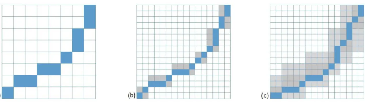
Constraints are widely used to speed up dynamic time warping algorithm. The most commonly used ones is the Sakoe-Chiba band (symmetric and asymmetric) [SC71]; [SC78] and Itakura parallelogram [Ita75], which are shown in Figure 1.4.

Figure 1.4: Speed up DTW using constraints: (a)Sakoe-Chiba band (b)Asymmetric Sakoe-Chiba band (c)Itakura parallelogram

The cost matrix are filled by the DTW algorithm in the shaded areas around the diagonal. In this case, the algorithm finds the optimal alignment warp math through the constraints

(32)

window. However, the global optimal alignment path will not be found, if it is not fully inside the window.

The Sakoe-Chiba dynamic time warping (DTWsc) between two time series, which is the

most well-used constrained DTW, is defined by: dtwsc(xi, xj)def= min π∈A C_(π) C_(π)def₌ 1 |π| |π| $ k=1 w_π₁_(k),π₂_(k) ϕ(xi_π1(k), xj_π2(k)) = 1 |π| $ (t,t′_)∈π wt,t′ ϕ(x_it, x_jt′) where if |t − t′_{| < c then w}

t,t′ = 1, and else ∞. Function ϕ taken as the euclidean norm and

parameter c is the Sakoe-Chiba band width. Figure 1.5 shows examples of the cost matrix and the two constrained optimal alignment path between two sample time series.

Figure 1.5: The constrained optimal alignment path between two sample time series (Sakoe-Chiba band = 5 - left), (Itakura parallelogram - right)

Piecewise DTW

Piecewise Dynamic Time Warping (PDTW) [KP00], takes advantage of the fact that one can eﬃciently approximate most of the time series by a Piecewise Aggregate Approximation (PAA). Let xi = (xi1, xi2, . . . , xiT) be a time series sequence that we wish to reduce its

dimensionality to T′_{, where (1 ≤ T}′ _{≤ T ). A time series x}∗

i of length T′ is represented by

(33)

x∗ it= T ′ T T T ′t $ t′₌T T ′(t−1)+1 xit′

Simply, to reduce the data from T dimensions to T′ dimensions, the data is divided into T′ frames with equal size. The average value of the data falling within each frame is computed and a vector of these values becomes the data reduced representation. The compression rate c (c = _TT′) is equal to the ratio of the length of the original time series to the length of

its PAA representation. Choosing a value for c, is a trade-oﬀ between memory savings and accuracy [KP00]. Figure 1.6 illustrates a time series and its PAA approximation.

x∗_i xi

Figure 1.6: The time series sequence xi, and its PAA x∗i

Finally, Figure 1.7 illustrates strong visual evidence that PDTW finds alignment that are very similar to those produced by DTW. Hence, the time complexity for PDTW is O(T′2), which means the speedup obtained by PDTW should be _O(TO(T′22)₎ which is O(c2).

Figure 1.7: Alignment between two time series by (a)DTW (b)PDTW

Therefore, piecewise method by finding a time series which is most similar to a given one, significantly speed up many DTW applications by reducing the number of times which the DTW should be run.

MultiScale DTW (FastDTW)

To obtain an eﬃcient as well as robust algorithm to compute DTW-based alignments, one can combine the global constraints and dimensionality reduction strategies in some iterative approaches to generate data-dependent constraint regions. The general strategy of multiscale DTW (or FastDTW)[SC04] is to recursively project a warping path computed at a coarse resolution level to the next level and then refine the projected warping path. Multiscale DTW or fastDTW speeds up the dynamic time warping algorithm by running DTW on a reduced representation of the data.

(34)

Let xi = (xi1, ..., xiT) and xj = (xj1, ..., xjT) be the sequences to be aligned, having

lengths T . The aim is to compute an optimal warping path between two time series xi

and xj. The highest resolution level will be called as Level 1. By reducing the feature

sampling rate by a factor of f , one achieves time series of length T_f. Next, one computes an optimal alignment warping path between two dimension-reduced time series on the resulting resolution level (Level 2). The obtained path is projected onto highest level (Level 1) and it defines a constraint region R. Lastly, an optimal alignment warping path relative to the restricted area R is computed. In general, the overall number of cells to be computed in this process is much smaller than the total number of cells on Level 1 (T2). The constrained warping path may not go along with the optimal alignment warping path. To mitigate this problem, one can increase the constraint region R by adding δ cells to the left, right, top and bottom of every cell in R. The resulting region Rδ will be called as δ-neighborhood of R [ZM06]. Figure 1.8 demonstrates an example of multiscale DTW for alignment two time series in the direction of reduce time and space complexity.

Figure 1.8: (a) The optimal alignment warp path on level 2. (b) The optimal alignment warp path with respect to the constraint region R by projecting alignment path to level 1. (c) The optimal alignment warp path with δ = 2

Finally, in spite of the great success of DTW and its variants in a diversity of domains, there are still several persistent myths about it, as finding ways to speed up DTW with no (or relaxed) constraints.

1.3.2 Behavior-based metrics

The second category of time series metrics concerns behavior-based metrics, where time series are compared according to their behaviors regardless of their values. That is the case when time series of a same class exhibit similar shape or behavior, and time series of different classes have different shapes. Hence, comparing the time series on the base of their value may not be valid assumption. In this context, we should define which time series are more similar together and which ones are different. The definition of similar, opposite and different behaviors are given as following.

Similar Behavior. Time series xi, xj are of similar behavior, if for each period [ti, ti+1],

(35)

Opposite Behavior. Time series xi, xj are of opposite behavior, if for each period

[ti, ti+1], i ∈ {1, ..., T }, when one time series increases, the other decreases with the same

growth rate in absolute value and vice-versa.

Diﬀerent Behavior. Time series xi, xj are of diﬀerent behavior, if they are not similar

nor opposite (linearly and stochastically independent).

Main techniques to recover time series behaviors are: slopes and derivatives comparison, ranks comparison, Pearson and temporal correlation coeﬃcient, and diﬀerence between auto-correlation operators. In the following, we briefly describe some well-used behavior-based metrics.

1.3.2.1 Pearson CORrelation coeﬃcient (COR)

Let X = {x1, ..., xN} be a set of time series xi = (xi1, ..., xiT) , i ∈ {1, ..., N }. The correlation

coeﬃcient between sequences xi and xj is defined by:

cor(xi, xj) = T $ t=1 (xit− xi)(xjt− xj) ! " " # T $ t=1 (xit − xi) 2 ! " " # T $ t=1 (xjt− xj) 2 (1.2) and xi = _T1 T $ t=1 xit

Correlation coefficient was first introduced by Bravais and later shown by Pearson [Pea96] to be the best possible correlation between two time series. Till now, many applications in different domains such as speech recognition, system design control, functional MRI and gene expression analysis have used the Pearson correlation coefficient as a behavior proximity measure between time series sequences [Mac+10]; [ENBJ05]; [AT10]; [Cab+07]; [RBK08]. The Pearson correlation coefficient changes between −1 and +1. The case COR = +1, called perfect positive correlation, occurs when two time series sequences perfectly coincide, and the case COR= −1, called the perfect negative correlation, occurs when two time series behave completely opposite. COR= 0 shows that the time series sequences have different behavior. Note that the higher correlation doesn’t conclude the similar dynamics.

(36)

1.3.2.2 Temporal CORrelation coeﬃcient (CORT)

To cope with temporal data, a variant of Pearson correlation coefficient, considering temporal dependency within r, is proposed in [DCA12], called as Temporal CORrelation coefficient (CORT). The authors considered an equivalent formula for the correlation coefficient relying on pairwise values differences as:

cor(xi, xj) = $ t,t′ (xit − xit′)(xjt− xjt′) +$ t,t′ (xit− xit′) 2+$ t,t′ (xjt− xjt′) 2 (1.3)

One can see that the Pearson correlation coefficient assumes the independence of data as based on the differences between all pairs of observations at [t, t′]; unlike, the behavior proximity needs only to capture how they behave at [t, t + r]. Therefore, the correlation coefficient is biased by all of the remaining pairs of values observed at interval [t, t′] with |t − t′| > r, r ∈ [1, ..., T − 1]. Temporal correlation coefficient defined as:

cort(xi, xj) = $ t,t′ mtt′(x_i_t − x_i t′)(xjt− xjt′) +$ t,t′ mtt′(x_i_t− x_i t′) 2+$ t,t′ mtt′(x_j_t − x_j t′) 2 (1.4)

where mtt′ = 1 if |t − t′| ≤ r, otherwise 0. CORT belongs to the interval [−1, +1]. The value

CORT(xi, xj) = 1 means that in any observed period [t, t′], xi and xj have similar behaviors.

The value CORT(xi, xj) = −1 means that in any observed period [t, t′], xi and xj have

opposite behaviors. Lastly, CORT(xi, xj) = 0 indicates that the time series are stochastically

linearly independent. Temporal correlation is sensitive to noise. So, the parameter r can be learned or fixed a priori, and for noisy time series higher value of r is advised.

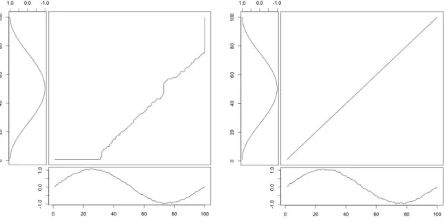
Figure 1.9 illustrates the comparison of the Pearson correlation coeﬃcient and the temporal correlation coeﬃcient between three samples time series.

Figure 1.9: Example of comparison of COR vs CORT (r = 1). COR(x1, x2) = – 0.90, COR(x1, x3)

(37)

1.3.2.3 Diﬀerence between Auto-Correlation Operators (DACO)

Auto-correlation is a representation of the degree of similarity which measures the dependency between a given time series and a shifted version of itself over successive time intervals. Let X = {x1, ..., xN} be a set of time series xi = (xi1, ..., xiT) i ∈ {1, ..., N }. The DACO between

the two time series xi and xj defined as [GHS11]:

daco(xi, xj) = ∥˜xi− ˜xj∥2 (1.5) where, ˜ x_i _{= (ρ}₁_(x_i_{), ..., ρ}_k_(x_i₎₎ and ρτ(xi) = T −τ $ t=1 (xit − xi)(xi(t+τ )− xi) T $ t=1 (xit − xi) 2

and τ is the time lag. Therefore, DACO compares time series by computing the distance between their dynamics, modeled by the auto-correlation operators. Note that the lower DACO doesn’t represent the similar behavior.

1.3.3 Combined (Behavior-value-based) metrics

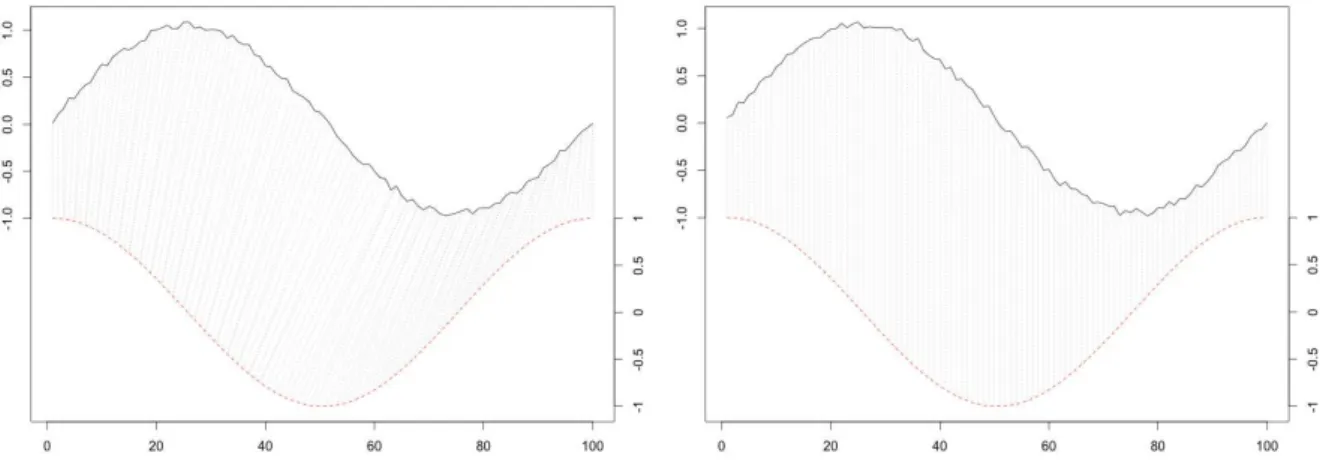
Considering the definition of time series basic metrics, the value-based one is based on the diﬀerences between the values of the time series and does not consider the dynamics and behaviors within the time series. Figure 1.10 shows two configurations: the left side, two time series x1 and x2 are definitely opposed, a decrease of one corresponding to a growth of the

other and vice-versa. While the right side, the two series x1 and x3 are in the same direction,

but have variations in intensity and scale. However, the overall behavior is similar. But, according to the definition of a value-based metrics, the time series x1 and x2 in left, have the

same distance (in Euclidean) with the two time series x1 and x3 in right.

Figure 1.10: Comparison of time series: similar in value, opposite in behavior (left), similar in behavior (right)

(38)

1.4. Kernels for time series 21

Most of the time, two time series sharing same configuration are considered close, even though they have very diﬀerent values, and vice-versa. Hence, choosing a proper metric can be crucial and very important for the time series comparison. In some cases, several behavior and value-based metrics may be implied. Some propositions show the benefit of involving both behavior and value-based metrics through a combination function. Therefore, to compare the time series and define a proximity measure covering both the behaviors and values components, a weighted linear (or geometric) function combines behavior and value-based metrics. In this context, they could be shown as:

BVLin(xi, xj) = α.V(xi, xj) + (1 − α).B(xi, xj)

BVGeom(xi, xj) = (V(xi, xj))α . (B(xi, xj))(1−α)

where V and B is a value-based and behavior-based metrics, respectively. The parameter α ∈ [0, 1] is a trade-oﬀ between the behavior and value-based components.

On the other hand, a time series may be considered in the spectral representations, which means the time series may be similar because they share the same frequency characteristics. Hence, in some application, the frequential-based metrics (e.g. wavelet transforms, fourier transforms) will be used. More specific works to combine two diﬀerent metrics through a combination function proposed in [DCN07]; [DCA12].

1.4 Kernels for time series

Over the last ten years estimation and learning methods using kernels have become rather popular to cope with non-linearities, particularly in machine learning. Kernel methods [HSS08] have been proved useful to handle and analyze structured data such as images, graphs and texts. They map the data from the original space (i.e. input space) via a nonlinear mapping function Φ(.) to a higher dimensional feature space (i.e. Hilbert space), to discover nonlinear patterns (see Figure 1.11). These methods formulate learning problems, in a reproducing kernel Hilbert space, of functions defined on the data domain expanded in terms of a kernel. < Φ(xi), Φ(xj) > = κ(xi, xj) < xi, xj> Linearly separable Φ(x) Feature Space Original Space Linearly non-separable

(39)

Usually, a kernel function κ(xi, xj) is used to directly provide the inner products in a

feature space without explicitly defining transformation. The kernel corresponds to the dot product in a (usually high-dimensional) feature space. In this space, the estimation methods are linear, but as long as we can formulate everything in terms of kernel evaluations, we explicitly never have to compute in the high-dimensional feature space. Such inner products can be viewed as measuring the similarity between samples. Let X = {x1, ..., xN} a set of

samples.

Gram matrix (or kernel matrix) of function κ with respect to the {x1, ..., xN} is a

N × N matrix defined by:

K := [ κ(xi, xj) ]_ij

where κ is a kernel function. If we use algorithms that only depend on the Gram matrix, K, then we never have to know (or compute) the actual features Φ. This is the crucial point of kernel methods.

Positive definite matrix is a real N × N symmetric matrix, that Kij satisfying:

$

i,j

cicjKij > 0

for all ci ∈R.

Positive semidefinite matrix is a real N × N symmetric matrix, that the Gram matrix Kij satisfying:

$

i,j

cicjKij ≥ 0

for all ci ∈R. In the following, to simplify, will call them definite. if we really need > 0, we

will say strictly positive definite.

A symmetric function κ : X × X →R which for all xi ∈ X, ∀i ∈ {1, ..., N } gives rise to a

positive definite Gram matrix is called a Positive definite kernel.

For time series, several kernels are proposed in the last years, properties of which will be discussed later. Ideally, a useful kernel for time series should be both positive definite and able to handle time series of structured data. Here, we refer positive definite kernels as kernels. Note that, for simplicity, we have restricted ourselves to the case of real valued kernels. The linear kernel is the simplest kernel function. It is given by the inner product < xi, xj > plus an optional constant γ. A polynomial kernel allows us to model feature

conjunctions up to the order of the polynomial, whereas the Gaussian kernel is an example of Radial Basis Function (RBF) kernel. In Table 1.1, some kernel function examples are given.

(40)

Linear Kernel κ(xi, xj) = (xTi xj+ γ)

Polynomial Kernel κ(xi, xj) = (α.xTi xj+ γ)δ

Gaussian Kernel κ(xi, xj) = exp(||xi−xj||

2

−2σ2 )

Table 1.1: Kernel function examples

The adjustable parameters σ, α, γ play a major role in the performance of the kernel, and should be carefully tuned to the problem at hand. In the following, diﬀerent methods to compute the kernel similarity Gram matrix presented.

1.4.1 Temporal correlation coeﬃcient kernel (κCORT)

cort(xi, xj), which is a behavior-based metric between two time series xiand xj and described

in Section 1.3.2.2, is a linear kernel and κCORT defined as a positive definite linear kernel as

following:

κCORT(xi, xj) = cort(xi, xj) = < △xi , △xj >

It is easy to prove that κCORT(xi, xj) can be constructed from inner products in appropriate

Hilbert spaces.

1.4.2 Auto-correlation kernel (κDACO)

To compare the dynamics of two actions Gaidon [GHS11] proposed to compute the distance between their respective auto-correlations. This distance is defined as the Hilbert-Schmidt norm of the diﬀerence between auto-correlations detailed in Section 1.3.2.3, and called as associated Gaussian RBF kernel "Diﬀerence between Auto-Correlation Operators Kernel". κDACO is defined by:

κDACO(xi, xj) = e

, −1

σ2daco(xi, xj)

-κDACO is a positive definite Gaussian kernel, designed specifically for action recognition.

Notice that, both κCORT and κDACOare temporal kernels under Euclidean alignments. Under

time warp, time series should be first synchronized by dtw, then kernels applied. In the following, we introduce the major well-known temporal kernels under dynamic time warping alignment.

(41)

1.4.3 Gaussian dynamic time warping kernel (κGDTW)

Following [BHB02], the dynamic time warping distance can be used as a pseudo negative definite kernel to define a pseudo positive definite kernel. κGDTW is determined by:

κGDTW(xi, xj) = e

, −1

t dtw(xi, xj)

-and using Sakoe-Chiba constrained dynamic time warping distance, κGDTWsc is defined by:

κGDTWsc(xi, xj) = e

, −1

t dtwsc(xi, xj)

-where t is a normalization parameter, and sc is a Sakoe-Chiba band. As the DTW is not a metric (invalid triangle inequality), one could fear that the resulting kernel lacks some necessary properties. Hence, general positive definiteness can not be proven for κGDTW, as

simple counterexamples can be found. However, this kernel can produce good results in some cases [HK02]; [DS02], but a problem of this approach is the quadratic computational complexity [BHB02].

1.4.4 Dynamic time-alignment kernel (κDTAK)

The Dynamic Time-Alignment Kernel (κDTAK) proposed in [Shi+02] adjusts another similarity

measure between two time series by considering the arithmetic mean of the kernel values along the alignment path. κDTAK, a pseudo positive definite kernel , is then defined by:

κDTAK(xi, xj) = max π∈A C(π) where, C(π) = 1 |π| |π| $ l=1 φ(xiπ1(l), xjπ2(l)) = 1 |π| |π| $ (t,t′_)∈π φ(xit, xjt′) and φ(xit, xjt′) = κ_σ(x_it, x_jt′) = e , −1 σ2 ∥xit− xjt′∥ 2

-Dynamic time-alignment kernel function is complicated and diﬃcult to analyze because the input data is a vector sequence with variable length and non-linear time normalization is embedded in the function. It performs DTW in the transformed feature space and finds the optimal path that maximizes the accumulated similarity. Indeed, the local similarity used for the κGDTW is the Euclidian distance, whereas the one used in κDTAK is the Gaussian

kernel value. κDTAK is a symmetric kernel function, however, in general, it may still be a

non positive definite kernel. Note that, in practice, several ad-hoc methods (e.g. perturb the whole diagonal by the absolute of the smallest eigenvalue) are used to ensure the positive definiteness, when the Gram matrix is not positive definite.

(42)

1.4.5 Global alignment kernel (κGA)

In kernel methods, both large and small similarities matter, they all contribute to the Gram matrix. Global Alignment kernel (κGA) [Cut+07] is not based on an optimal path chosen given

a criterion, but takes advantage of all score values spanned by all possible alignments. The κGA which is positive definite under mild conditions2, seems to do a better job of quantifying

all similarities coherently, because it considers all possible alignments. κGA is defined by:

κGA(xi, xj) = $ π∈A |π| . l=1 k(x_iπ₁_(l), x_jπ₂_(l))

where k(x, y) = e−λΦσ(x,y)_{, factor λ > 0, and}

Φσ(x, y) =

1

2σ2∥x − y∥

2_{+ log(2 − e}_2σ2−1∥x−y∥2

)

In the sense of kernel κGA, two sequences are similar not only if they have one single

alignment with high score, which results in a small DTW distance, but also share numerous eﬃcient and suitable alignments. Hence, the function Φσ is a negative definite kernel, it can be

scaled by a factor λ to define a local positive definite kernel e−λΦσ_{. Global alignment kernels}

have been relatively successful in diﬀerent application fields [JER09]; [RTZ10]; [VS10] and shown to be competitive when compared with other kernels. However, similar to the κGDTW

and κDTAK kernels, it has quadratic complexity, O(pT2), where T is the length of time series

and p denotes the complexity of the measure between aligned instants.

1.4.6 Triangular global alignment kernel (κTGA)

The idea of Sakoe-Chiba [SC78], to speed up the computation of DTW, applied to the κGA to

introduce fast global alignment kernels, named as Triangular Global Alignment kernels. κTGA

kernel [Cut11] considers a smaller subset of such alignments rather than κGA. It is faster to

compute and positive definite, and can be seen as trade-oﬀ between the full κGA (accurate

but slow) and a Sakoe-Chiba Gaussian kernel (fast but limited). This kernel is defined by:

κTGA(xi, xj) = $ π∈A |π| . l=1 k(x_iπ₁_(l), x_jπ₂_(l)) k(x_iπ₁_(l), x_jπ₂_(l)) = wπ1(l),π2(l)kσ(xiπ1(l), xjπ2(l)) 2 − wπ1(l),π2(l)kσ(xiπ1(l), xjπ2(l))

where, w is a radial basis kernel in R (a triangular kernel for integers):

w(t, t′) = / 1 −|t − t ′_| c 0 2_κ

(43)

which guarantees that only the alignments π that are close to the diagonal are considered and the parameters c is the Sakoe-Chiba bandwidth. Note that as c increases the κTGA converges

to the κGA.

In fact, many generic kernels (e.g. Gaussian kernels), as well as very specific ones, describe diﬀerent notions of similarity between time series, which do not correspond to any intuitive or easily interpretable high-dimensional representation. They can be used to compute similarities (or distances) in feature spaces using the mapping functions. Precisely, the class of kernels that can be used is larger than those commonly used in the kernel methods which known as positive definite kernels.

1.5 Conclusion

A large variety of real world applications, such as meteorology, geophysics and astrophysics, collect observations that can be represented as time series. Time series data mining and time series analysis can be exploited from research areas dealing with sequences and signals, such as pattern recognition, image and signal processing. The main problem that arises during time series analysis is comparison of time series.

There has been active research on quantification of the "similarity", the "dissimilarity" or the "distance" between time series. Even, looking for the patterns and dependencies in the visualizations of time series can be a very exhausting task and the aim of this work is to find the more similar behavior time series, while the value-based proximity measures are the most studied approaches to compare the time series. Most of the time, two time series sharing same configuration are considered close, even they have very diﬀerent values, their appearances are similar in terms of form. In both comparison metrics, a crucial question is establishing what we mean by "similar" or "dissimilar" time series due to the dynamic of the series (with or without considering delay).

To handle and analysis non-linearly structured data, a simple way is to treat the time series as vectors and simply employ a linear kernel or Radial basis function kernel. For this, diﬀerent kernels have been proposed. To discover non-linear patterns, they map the data from the original input space to a higher dimensional feature space, called Hilbert space. They can be used to compute similarity between the time series. Ideally, a useful kernel for time series should be positive definite and able to handle the temporal data. Notice that, the computational complexity of kernel construction and evaluation can play a critical role in applying kernel methods to time series data.

In summary, finding a suitable proximity measure is a crucial aspect when dealing with the time series (e.g. a kernel similarity, a similarity or dissimilarity measure, a distance), that captures the essence of the time series according to the domain of application. For example, Euclidean distance is commonly used due to its computational eﬃciency; however, it is very brittle for time series and small shifts of one time series can result in huge distance changes. Therefore, more sophisticated distances have been devised to be more robust to small

(44)

1.5. Conclusion 27

fluctuations of the input time series. Notably, Dynamic Time Warping (DTW) has enjoyed success in many areas where its time complexity is not an issue. Using the discussed distances and (dis)similarity proximity measures, we will be able to compare time series and analyze them. This can provide useful insights on the time series, before the averaging and centroid estimation step. In the next chapter, we will discuss about averaging time series problems, diﬃculties and complexities.

(45)

(46)

Chapter 2

Time series averaging and centroid

estimation

Sommaire 2.1 Introduction . . . 29 2.2 Consensus sequence . . . 31 2.2.1 Medoid sequence . . . 31 2.2.2 Average sequence . . . 32 2.3 Multiple temporal alignments . . . 32 2.3.1 Dynamic programming . . . 33 2.3.2 Progressive approaches . . . 33 2.3.3 Iterative approaches . . . 36 2.4 Conclusion . . . 37

Averaging a set of time series, under the frequently used dynamic time warping, needs to address the problem of multiple temporal alignments, a challenging issue in various domains. Under temporal metrics, one standard way to average two time series is to synchronize them and average each pairwise temporal warping alignment. To average more than two time series, the problem becomes more complex as one needs to determine a multiple alignment that link simultaneously all the time series on their commonly shared similar elements. In this chapter, we present initially the definition of a consensus sequence and multiple temporal alignment problems, then we review major progressive and iterative centroid estimation approaches under time warp, and discuss their properties and complexities.

2.1 Introduction

Estimating the centroid of a set of time series is an essential task of many data analysis and mining processes, as summarizing a set of time series, extracting temporal prototypes, or clustering time series. Averaging a set of time series, under the frequently used dynamic time warping [KL83]; [SK83] metric or its variants [Ita75]; [Rab89]; [SC78], needs to address the tricky multiple temporal alignments problem, a challenging issue in various domains.