HAL Id: hal-01764470
https://hal.archives-ouvertes.fr/hal-01764470
Submitted on 12 Apr 2018
HAL is a multi-disciplinary open access
archive for the deposit and dissemination of
sci-entific research documents, whether they are
pub-lished or not. The documents may come from
teaching and research institutions in France or
abroad, or from public or private research centers.
L’archive ouverte pluridisciplinaire HAL, est
destinée au dépôt et à la diffusion de documents
scientifiques de niveau recherche, publiés ou non,
émanant des établissements d’enseignement et de
recherche français ou étrangers, des laboratoires
publics ou privés.
A Multi-wall and Multi-frequency Home Environment
Path Loss Characterization and Modeling
M Kacou, V. Guillet, Ghaïs El Zein, Gheorghe Zaharia
To cite this version:
M Kacou, V. Guillet, Ghaïs El Zein, Gheorghe Zaharia. A Multi-wall and Multi-frequency Home
Environment Path Loss Characterization and Modeling. 12th European Conference on Antennas and
Propagation (EUCAP 2018), Apr 2018, Londres, United Kingdom. �10.1049/cp.2018.0464�.
�hal-01764470�
A Multi-wall and Multi-frequency Home
Environment Path Loss Characterization and
Modeling
M. KACOU
1, V. GUILLET
1, G. EL ZEIN
2, G. ZAHARIA
21 Orange Labs, 1 Rue Louis et Maurice de Broglie, 90000 Belfort, France, {marc.kacou;valery.guillet}@orange.com 2 IETR-UMR 6164, INSA, 20 av. des buttes de Coësmes, CS 70839, 35708 Rennes, France
Abstract—Multi-technology wireless networks enable the
combination of the strength and usage of different wireless systems such as Wi-Fi, mobile and IoT networks. The design of such networks requires primarily the study of the radio coverage of wireless technologies that, most of the time, operate in different frequency bands. For this purpose, this paper presents a multi-wall and multi-frequency indoor path loss model based on measurements performed from 800 MHz to 6 GHz in the same residential environment. The presented results are focused on the carrier frequency effect and on the level of details of the building representation.
Index Terms—path loss, multi-wall model, residential
environment.
I. INTRODUCTION
Going from public environments like offices to more private ones such as residential places, wireless networks are used everywhere. There is a correlation between the frequency band in which a wireless system operates and its applications. For instance, at 5 GHz, bandwidth and throughput put aside, the shorter radio coverage may be a great asset for security purpose. Nowadays, it becomes possible to integrate into a single access point heterogeneous wireless technologies like IoT, Wi-Fi (2.4-5-60 GHz) and mobile technologies (2G/3G/4G, 5G in the future). Being able to combine the strength and usage of these different wireless technologies is the key point in designing a multi-technology wireless network.
Such task requires the study of the coverage area of the different wireless systems. For this purpose, deterministic or empiric path loss models can be used as references. The deterministic models are based on the process of accurate information such as the structure of the environment and the presence of furniture. They produce good results without having to perform any measurement but the main drawback is the high computational power needed. On the other hand, empiric path loss models are less accurate but provide a very low processing time. They are established by processing the path loss between a transmitter and a receiver taking into account different parameters such as the distance between them, and to some extent, the number of building obstacles (walls, floors …) crossed by the direct line between the transmitter and the receiver.
In the literature, there are several works related to the path loss modeling based on measurement campaigns. [1], [2] and [3] present log-distance path loss models available at 2.4, 5 and 60 GHz for residential environments. There exist other models covering a wider frequency range under 6 GHz. [4] and [5] introduce different path loss models available from 900 MHz to 6 GHz for environment having only one room like classrooms, etc. Other models take into account the multi-room parameter such as [1] and [6] which present different multi-stage path loss models for professional, residential and commercial environments. While these models are fully established from 900 MHz to 60 GHz for professional and commercial indoor environments, the models for residential environments are only available around 2.4 and 5 GHz. By combining the results of these works, it would be possible to obtain path loss models for residential environments covering the 0.8-6 GHz band. The main issue by doing so is the coherence of the results since the measurements were taken at different places and probably with different antenna characteristics as well.
The objective of this paper is to propose empiric path loss models applicable from 800 MHz to 6 GHz for multi-room residential environment based on measurements performed at the same locations with the same wideband antennas.
The rest of this paper is organized as follows. Section II describes the measurement environment, the measurement setup and the measurement procedure. In Section III the different path loss models are presented and fully analyzed. Section IV describes additional results such as the effect of the carrier frequency and transmitter’s antenna height on the path loss. Finally, conclusions are drawn in Section V.
II. INDOOR PROPAGATION MEASUREMENT
A. Measurement Environment
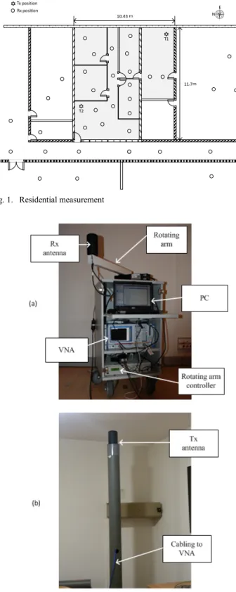
The measurements are carried out in a multi-room residential environment as shown in Fig. 1. Its size is about 10.4 x 11.7 x 2.6 m3. The windows are located only on the
east side of the apartment. There are different kinds of walls as shown in Table I, and most of them are load bearing walls with various thicknesses (14 to 60 cm). The apartment is not empty; there are also wooden furniture such as tables,
closet (trunk, chest) etc. that are not represented on Fig. 1 for the sake of clarity. No people were present in the environment during the measurements.
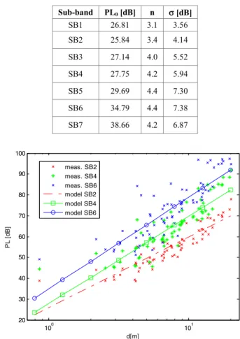
B. Measurement System Setup
The measurement system is displayed in Fig. 2. It is composed of the transmitting (Tx) and receiving (Rx) antennas that are both 2-dBi gain omnidirectional vertically polarized dipole antennas (ref: COBHAM XPO2V-0.8/6.0/1485).
A vector network analyzer (VNA) measures the S21 parameter over 512 sub-carriers sequentially in 7 frequency sub-bands (SBs) below 6 GHz. These bands correspond to different technologies as indicated in Table II. SB1 and SB2 have a bandwidth lesser than 100 MHz because of the lack of interference-free radio channels for higher bandwidths. Widebands are considered for further multipath analysis, but they provide also more accurate average path loss estimations, thanks to reduced small-scale fading compared to narrowband measurements.
A laptop commands the VNA and the rotating arm controller for the receiving antenna. It is also used to collect the measured data.
The Tx antenna is connected to the VNA’s output via a 25-metercoaxial cable and the Tx power is 13 dBm at the VNA’s output. At the receiving side a 25 dB low noise amplifier is used.
C. Measurement Procedure
On the transmitter side, 2 positions are chosen. T1 is located in the furthest room and T2 is placed in the main room of the apartment. For each Tx position, there are 4 antenna heights. Each height corresponds to a particular use case:
• Tx near an electrical outlet (hTx = 0.23 m), • Tx on a desk (hTx = 1.03 m),
• Tx on a closet (hTx = 1.67 m), • Tx near the ceiling (hTx = 2.3 m).
On the receiver side, 19 positions are chosen inside the apartment and 16 positions outside, precisely in nearby rooms or corridors. The Rx antenna height is equal to 1.2 m for all these 35 Rx positions.
At each Rx position, a rotation measurement is performed. Indeed, the Rx antenna is placed on a rotating arm having a radius of 56 cm. That arm rotates in azimuth from 0° to 360° with a step size of 6°. At each of the 60 angular steps, measurements are performed by the VNA over the 7 frequency sub-bands.
The circumference around each Rx position is at least 10 times greater than the greatest wavelength (λSB1) to get an
estimated average path loss value at each Rx position for each sub-band.
Fig. 1. Residential measurement
TABLE I. DIFFERENT KINDS OF WALLS
Legend Label Description Thickness (cm)
Mat0 Wall with windows 7,5 Mat1 Wooden door 4 Mat2 Load-bearing wall 1 28 Mat3 Load-bearing wall 2 24 Mat4 Plasterboard 7 Mat5 Concrete wall 3 14 Mat6 Load-bearing wall 4 56 Mat7 Load-bearing wall 5 23 Mat8 Load-bearing wall 6 52 TABLE II. TARGET FREQUENCY BANDS
Sub-band Frequency range (MHz) Bandwidth (MHz) technology Radio
SB1 864 – 884 20 IoT SB2 968 – 1024 56 2G SB3 1980 – 2080 100 DECT SB4 2400 – 2500 100 Wi-Fi SB5 3600 – 3700 100 5G (?) SB6 5250 – 5350 100 Wi-Fi SB7 5500 – 5600 100 Wi-Fi
III. INDOOR PATH LOSS MODELS
This section presents three path loss models for each of the 7 sub-bands. The first one is a log-distance model and the following ones are multi-wall models [7]. The parameters of these models are obtained by performing series of multiple linear regressions between the measured path loss and the variables of interest.
It is also worth to mention that the path loss estimated is actually the transmission path loss because it includes the gain of the Tx and Rx antennas. The effect of other components such as the coaxial cable or the amplifier at Rx have been calibrated and removed during the data processing.
The results are available for hTx=2.3 m. The transmitter’s
height impact on path loss is studied in a further section (IV).
A. Log-distance Path Loss Model
A path loss model over distance can be described by the following model:
PL(d) [dB] = PL0(d0) + 10nlog10(d/d0) + Xσ (1)
where PL(d) is the path loss value at a Tx-Rx distance equals to d, PL0(d0) is the path loss at a reference distance
d0, n is the path loss exponent that depends on the environment and characterizes the increase of the path loss
with distance. Xσ reflects the other variation of the path loss caused by shadowing effects and multiple paths. It is a zero-mean Gaussian random variable with a standard deviation of σ dB.
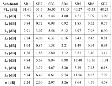
For d0 = 1 m, Table III summarizes the model parameters deduced from the measurement campaign and Fig. 3 shows some example of path loss versus distance for SB2, SB4 and SB6. The path loss exponent and σ increase with the carrier frequency.
B. Multi-wall Path Loss Model
The multi-wall model expressed by (2) gives the path loss in environment where the direct line between Tx and Rx crosses several kinds and amounts of walls added to the free space log distance path loss.
PL(d) [dB] = PL0(d0) + 20log10(d/d0) + Σ kiLi+ Xσ (2)
PL(d) is the path loss value at a Tx-Rx distance equal to d, PL0(d0) is the path loss at a reference distance d0 equal to 1 m, M is the total number of kinds of wall, ki is the number of walls of type i crossed by direct line between Tx and Rx, Li is the penetration loss of the type i walls and Xσis a zero-mean Gaussian random variable with a standard deviation of σ dB.
TABLE III. PARAMETERS OF THE LOG-DISTANCE PATH LOSS MODEL PER SUB-BAND
Sub-band PL0 [dB] n σ [dB] SB1 26.81 3.1 3.56 SB2 25.84 3.4 4.14 SB3 27.14 4.0 5.52 SB4 27.75 4.2 5.94 SB5 29.69 4.4 7.30 SB6 34.79 4.4 7.38 SB7 38.66 4.2 6.87 100 101 20 30 40 50 60 70 80 90 100 d[m] PL [ d B] meas. SB2 meas. SB4 meas. SB6 model SB2 model SB4 model SB6
Fig. 3. Path loss measurements and model for SB2, SB4 and SB6
M
For each sub-band, two multi-wall path loss models are established. The main difference between them is the level of details considered to represent the building materials: the first one is said to be generalized while the second one is more detailed.
1) Generalized multi-wall path loss model: For this
model, the different kinds of wall shown in Table II are divided into two groups. The first one is the dividing wall (DW) group which is a collection of the non load-bearing walls (Mat0, Mat1 and Mat4). The second one is the load-bearing wall (BW) group which concerns the load-load-bearing walls (Mat2, Mat3, Mat5, Mat6, Mat7 and Mat8).
The results given in Table IV show that the path loss increases with the carrier frequency and the load bearing walls play a major role in this growth. Indeed, from 860 MHz to 6 GHz the loss of the DW group remain inferior to 2dB while the loss cause the BW group varies from 3 to 8 dB.
TABLE IV. PARAMETERS OF THE GENERALIZED MULTI-WALL PATH LOSS MODEL PER SUB-BAND
Sub-band PL0 [dB] LDW [dB] LBW [dB] σ [dB] SB1 31.42 1.03 3.07 2.99 SB2 31.36 0.99 4.14 3.10 SB3 35.84 1.49 6.01 4.08 SB4 36.98 1.83 6.51 4.21 SB5 39.62 1.72 7.59 5.21 SB6 45.12 0.89 8.05 5.24 SB7 47.97 0.95 7.14 5.12
TABLE V. PARAMETERS OF THE DETAILED MULTI-WALL PATH LOSS MODEL PER SUB-BAND
Sub-band SB1 SB2 SB3 SB4 SB5 SB6 SB7 PL0 [dB] 31.61 31.6 36.05 37.15 40.27 45.33 48.23 L0 [dB] 3.59 3.31 5.44 4.80 4.21 3.09 3.09 L1 [dB] 0.84 0.72 0.98 0.92 1.85 0.52 0.77 L2 [dB] 2.91 3.07 5.56 6.12 6.97 7.98 6.90 L3 [dB] 2.24 4.06 6.31 6.16 6.43 9.43 8.81 L4 [dB] 1.04 0.86 1.58 2.21 1.49 0.94 0.93 L5 [dB] 1.28 1.88 2.80 3.12 3.57 3.40 3.17 L6 [dB] 4.84 5.68 8.94 9.98 13.40 13.30 11.91 L7 [dB] 1.86 3.79 4.67 5.26 5.19 7.43 6.18 L8 [dB] 5.74 6.49 8.61 9.74 11.96 8.83 7.92 σ [dB] 2.24 2.60 2.97 3.26 3.64 4.59 4.58
TABLE VI. STANDARD DEVIATION PER SUB-BAND OF THE THREE PROPOSED PATH LOSS MODELS
Sub-band Log-distance model Generalized multi-walls model Detailed Multi-walls Model σ1[dB] σ1− σ3 σ2 [dB] σ2− σ3 σ3[dB] SB1 3.56 1.32 2.99 0.75 2.24 SB2 4.14 1.54 3.10 0.50 2.60 SB3 5.52 2.55 4.08 1.11 2.97 SB4 5.94 2.68 4.21 0.95 3.26 SB5 7.30 3.66 5.21 1.57 3.64 SB6 7.38 2.79 5.24 0.65 4.59 SB7 6.87 2.29 5.12 0.54 4.58
2) Detailed multi-wall path loss model: For this
model, the path loss computation takes into account all of the types of wall presented in Table II. This is not always possible in practice, as it is not easy to know exactly what are the buiding materials for any construction. However it is interesting to make such an analysis to get the impact of a simplified or a detailled representation on the model accuracy.
The results are shown in Table V and the conclusion is the same than in the generalized case. The path loss increases with the frequency and the load-bearing walls play a major role in this growth.
C. Comparison of the Models
Table VI indicates the standard deviation for each model per sub-band. The detailed multi-wall model is by far the most accurate in the estimation of the path loss. However as its name implies, there are a lot of parameters that must be taken into consideration. The generalized multi-wall model is less accurate than the detailed one, but is more simplified. The log-distance model is the least accurate of the three models but the most simplified one.
Regarding the previous observations, the generalized multi-wall model seems to be the “best” model because it achieves a great compromise between accuracy and simplification of the building’s map representation.
IV. ADDITIONAL RESULTS
A. Multi-frequency Path Loss Models
The results obtained in section III confirm that the path loss increases with the frequency. This section goes deeper and presents two path loss models that explicit this relationship. The first one derives from the log-distance path loss model presented in Table III and the second one from the generalized multi-wall path loss model described in Table IV.
1) Multi-frequency log-distance path loss model: The
path loss over distance can be described by the following model:
PL(d, f) [dB] = PL0(d0,f0) + 10nd log10(d/d0) + 10nf
log10(f/f0) + Xσ (3)
where PL(d,f) is the path loss value at a Tx-Rx distance equals to d and a frequency f (expressed in GHz), PL0(d0,f0)
is the path loss at a reference distance d0 and a reference frequency f0, nd is the path loss exponent over distance, nf is the path loss exponent over frequency, Xσ is a zero-mean Gaussian random variable with a standard deviation of σ dB. For d0 and f0 respectively equal to 1 m and 1 GHz, Table VII gives the parameters of the model.
2) Multi-frequency multi-wall path loss model: The
multi-wall model expressed by (4) gives the path loss in environment where the signal crosses two types of wall: dividing walls (DWs) and load-bearing walls (BWs) as indicated in section III.
PL(d, f) [dB] = PL0(d0,f0) + 20 log10(d/d0) + 10nf
log10(f/f0) + kDW LDW + kBW LBW + Xσ (4)
PL(d, f) is the path loss value at a Tx-Rx distance equals to d and a frequency f (expressed in GHz), PL0(d0,f0) is the path loss at a reference distance d0 and a reference frequency f0, nf is the path loss exponent over frequency, kg is the number of walls belonging to the group g crossed by direct line between Tx and Rx, Lg is the penetration loss of the group g walls and Xσ is a zero-mean Gaussian random
variable with a standard deviation of σ dB. For d0, f0 respectively equal to 1 m and 1 GHz, Table VII shows the parameters of the model.
3) Comparison of the models: The two models
demonstrate that the path loss increases with the frequency with the same exponent which is 2.5. The main difference between them lies in the estimation of the path loss. As it was observed in section III, the generalized multi-wall model seems to be the “best” model because it is more accurate and offer a relatively simplified representation of the building map.
B. Effect of the Tx Antenna Height
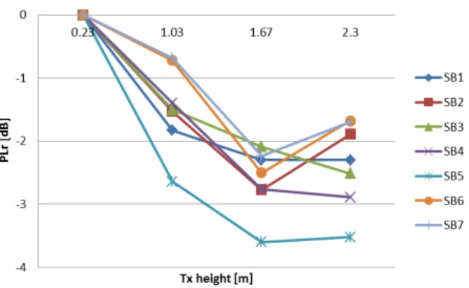
Since the results in section III are available for only one Tx height (hTx = 2.3 m), this section presents a brief study of the effect of the Tx antenna height on the average path loss. Fig. 4 illustrates for each sub-band the relative average path loss given by the following formula:
PLr[dB] (hTx) = PL(hTx) + σ(hTx) – PL(0.23) – σ(0.23) (5)
where PLr(hTx) is the relative path loss for a Tx height equal to hTx, PL(hTx) and σ(hTx) are respectively the average measured path loss for the 35 Rx and the standard deviation for a for a Tx height equal to hTx, PL(0.23) and σ(0.23) are
respectively the average measured path loss and the standard deviation for the reference Tx height equal to 0.23 m.
TABLE VII. PARAMETERS OF THE PROPOSED MULTI-FREQUENCY PATH LOSS MODELS Model PL0[dB] nd nf LDW[dB] LBW[dB] σ [dB] Log-distance model 20.36 4.0 2.5 - - 6.07 Multi-wall model 28.59 2.0 2.5 1.27 6.07 4.66
Fig. 4. Relative path loss per sub-band for each Tx height
The results display that the Tx antenna height has an effect on the path loss. Indeed, from hTx = 0.23 m to hTx = 2.30 m, there is global decrease of the path loss and the minimum “gain” due to the Tx antenna height is 1.7 dB. However, Fig. 6 reveals also that beyond a certain level (here hTx = 1.67 m) that gain grows marginally, probably due to some antenna directivity in elevation pattern.
V. CONCLUSION
This paper mainly presents two path loss models for multi-room residential environment from 800 MHz to 6 GHz. The first model is based on a log-distance approach and the second one is a multi-wall path loss model in which two kinds of walls are identified: load-bearing and non-load bearing walls. The results show that the multi-wall model is the “best” compromise in terms of accuracy and complexity.
ACKNOWLEDGMENT
This work was supported by the French project FUI22 OptimiSME and by the French BPI.
REFERENCES
[1] V.Guillet, “Narrowband and wideband characteristics of 60 GHz radio propagation in residential environment,” In Electronic Letters, vol. 37, No. 21, 2001.
[2] V. Erceg et al., “TGn channel models, ” in Technical Report Doc. : IEEE 802.11-03/940r4, IEEE P802.11 Wireless LANs, 2004. [3] “TGac Channel Model Addendum, ” IEEE 802.11-09/308r12. [4] S. Gen, J. Kivinen, X. Zhao and P. Vainikainen, “Millimeter-wave
propagation channel characterization for short-range wireless communications,” IEEE Transactions on Vehicular Technology, 58(1), 3-13, 2009.
[5] ITU-R, “ITU-R M.2135: Guidelines for evaluation of radio interface technologies for IMT-Advanced,” 2008.
[6] ITU-R, “Propagation data and prediction methods for the planning of indoor radiocommunication systems and radio local area networks in the frequency range 900 MHz to 100 GHz,” Recommendation ITU-R P.1328-7, 2012.
[7] A. G. M. Lima and L. F. Menezes, “Motley-Keenan model adjusted to the thickness of the wall,” in SBMO/IEEE MTT-S International Conference in Microwave and Optoelectronics, 2005, pp. 180-182.