THESIS SUBMITTED TO
ÉCOLE DE TECHNOLOGIE SUPÉRIEURE
IN PARTIAL FULFILLMENT OF THE REQUIREMENTS FOR THE DEGREE OF MASTER OF SCIENCE IN AUTOMATED PRODUCTION ENGINEERING
M.Eng.
BY
EMIL GABRIEL CRISAN
V ALIDA TION OF A MATHEMATICAL MO DEL FOR BELL 427 HELICOPTER USING PARAMETER ESTIMATION TECHNIQUES AND FLIGHT TEST DATA
Mme Ruxandra Botez, director of thesis
Department of Automated Production Engineering at École de technologie supérieure
M. Njuki Mureithi, co-director
Department of Mechanical Engineering at École Polytechnique de Montréal
M. Eric Granger, president of jury
Department of Automated Production Engineering at École de technologie supérieure
M. Joey Seto, external jury member
Aerodynamics and Handling Qualities Group, Bell Helicopter Textron Canada
THIS THESIS W AS PRESENTED IN FRONT OF JURY
ON
ih
of APRIL, 2005Emil Gabriel Crisan ABSTRACT
Certification requirements, optimization and minimum project costs, design of flight control laws and the implementation of flight simulators are among the principal applications of system identification in the aeronautical industry. This document examines the practical application of parameter estimation techniques to the problem of estimating helicopter stability and control derivatives from flight test data provided by Bell Helicopter Textron Canada.
The purpose of this work is twofold: a time-domain application of the Output Error method using the Gauss-Newton algorithm and a frequency-domain identification method to obtain the aerodynamic and control derivatives of a helicopter. The adopted madel for this study is a fully coupled, 6 degree of freedom (DoF) state space madel. The technique used for rotorcraft identification in time-domain was the Maximum Likelihood Estimation method, embodied in a modified version of NASA's Maximum Likelihood Estimator program (MMLE3) obtained from the National Research Council (NRC). The frequency-domain system identification procedure is incorporated m a comprehensive package ofuser-oriented programs referred to as CIFER®.
The coupled, 6 DoF madel does not include the high frequency main rotor modes (flapping, lead-lag, twisting), yet it is capable of modeling rotorcraft dynamics fairly accurately as resulted from the model verification. The identification results demonstrate that MMLE3 is a powerful and effective tool for extracting reliable helicopter models from flight test data. The results obtained in :frequency-domain approach demonstrated that CIFER® could achieve good results even on limited data.
Emil Gabriel Crisan SOMMAIRE
Les demandes de certification, d'optimisation et des coûts minimaux des projets, le design des lois de commande de vol et l'implantation des simulateurs de vol se trouvent parmi les applications principales de 1 'indentification des systèmes dans 1 'industrie aéronautique. Ce mémoire analyse l'application pratique des techniques d'estimation de paramètres aux problèmes d'estimation des dérivées de stabilité et contrôle à partir des données d'essais en vol fournies par Bell Helicopter Textron Canada.
Ce travail consiste en deux parties : l'application dans le domaine du temps de la méthode d'erreur de la sortie en utilisant l'algorithme de Gauss- Newton et la méthode d'identification dans le domaine de la fréquence pour l'obtention des dérivées aérodynamiques et de contrôle des hélicoptères. Le modèle utilisé dans l'étude est le modèle sous forme d'espace d'état en six degrés de liberté. La technique utilisée pour l'identification des hélicoptères dans le domaine du temps est la méthode d'estimation de probabilité maximale des paramètres (Maximum Likelihood Estimation method) et elle est incluse dans la version modifiée du programme d'estimation des paramètres de la NASA (Modified Maximum Likelihood Estimator program, MMLE3) obtenu de la part de National Research Council (NRC). La procédure d'identification des systèmes dans le domaine de fréquence est incorporée dans 1' ensemble des programmes orientés vers l'utilisateur et appelés CIFER®.
Le modèle en 6 degrés de liberté n'inclut pas les modes du rotor principal aux très hautes fréquences, mais la dynamique de 1 'hélicoptère est modélisée aussi précisément que celle calculée par la validation du modèle. Les résultats d'identification montrent que MMLE3 est un outil puissant et efficace pour 1' extraction des modèles d'hélicoptères à partir des données d'essais en vol. Les résultats obtenus par l'approche dans le domaine de fréquence montrent que CIFER ® peut donner des bons résultats même sur des données d'essais en vol limitées.
L'HÉLICOPTÈRE BELL 427 À PARTIR DES ESSAIS EN VOL
RÉSUMÉ
Introduction
Ce mémoire analyse l'application pratique des techniques d'estimation de paramètres aux problèmes d'estimation des dérivées de stabilité et contrôle à partir des données d'essais en vol fournies par Bell Helicopter Textron Canada. Le travail est concentré sur le calcul des dérivées de stabilité et contrôle de 1 'hélicoptère Bell 427 en utilisant un modèle sous forme d'espace d'état en 6 degrés en liberté. Ce modèle utilise des équations linéaires et couplées.
L'efficience des méthodes d'estimation des paramètres a été testée en comparant les données réelles des essais en vol avec les réponses prédites de 1 'hélicoptère. Deux approches ont été utilisées pour résoudre le problème d'identification : a) une application dans le domaine du temps de la méthode de 1' erreur de la sortie en utilisant l'algorithme de minimisation de Gauss - Newton et b) une méthode d'identification dans le domaine de la fréquence.
La sélection de l'entrée optimale
L'entrée de commande pour l'essai en vol a toujours un impact majeur sur la qualité des données recueillies pour la modélisation de la dynamique de 1 'hélicoptère. Pour le programme d'estimation des paramètres du modèle Bell 427, le mouvement de
longueurs différentes, et sont des entrées de contrôle de la forme 2311, où les chiffres expriment le nombre de périodes de temps unitaire (1 seconde) entre les inversions des signes des différents contrôles appliqués par le pilote.
Les avantages des entrées de contrôle 2311 sont : a. Le contenu en hautes fréquences suffisant;
b. La facilité d'exciter tous les modes de mouvement de l'avion; c. Une courte durée, facilement exécutable et répétable;
d. Pas d'excitation des modes du rotor de haute fréquence, qui ne sont pas inclus dans le modèle en six degrés de liberté.
Pendant 1' essai en vol, une seule entrée du contrôle à la fois a été utilisée pour exciter la réponse sur chaque axe de 1 'hélicoptère et pour éviter la corrélation avec les autres contrôles. Des conditions de vol dans l'air calme, sans turbulences, ont été considérées.
L'instrumentation de l'hélicoptère pendant les essais
La précision des paramètres estimés est dépendante de la qualité des données des essais en vol mesurées. Des mesures de grande précision des entrées de contrôle et des variables de mouvement sont nécessaires pour l'application des méthodes d'identification des paramètres.
Les données d'essais en vol de Bell 427 sont obtenues à l'aide des sous-systèmes suivants:
a. Un gyroscope laser pour les mesures des vitesses de roulis (p), tangage (q) et lacet (r), et pour des angles de roulis ( ~ ), de tangage ( e) et de lacet (If/) ;
b. Accéléromètres linéaires installés proche du centre de gravité CG de l'avion pour les mesures des accélérations longitudinales, latérales et verticales
(ax,ay,az);
d. Un dispositif pour les données de l'air équipé d'un capteur de pressiOn et ailettes pour les mesures suivantes : vitesse totale de l'air (V), angle d'attaque
(a ) et angle de dérapage ( f3 );
e. Un capteur de pression pour mesurer 1' altitude et le taux de montée; f. Un capteur de température pour mesurer la température extérieure (OAT); g. Un ordinateur de données de vol qui calcule la position de 1 'hélicoptère en
temps réel (à partir du système de positionnement global GPS) ainsi que le poids de l'hélicoptère et la position de son centre de gravité;
Toutes les données nécessaires pour l'estimation des paramètres ont été numérisées et enregistrées au bord de l'hélicoptère à un taux d'échantillonnage de 50 échantillons par seconde. Pendant les essais en vol, les signaux mesurés ont été envoyés par la télémétrie à la station au sol où la variation dans le temps des variables sélectionnées a été présentée sur des moniteurs et des chartes pour des vérifications rapides. Une réduction des données dans le temps réel a été réalisée pour isoler les inconsistances et les erreurs de transmission des données. En utilisant les vérifications des données en ligne, ensemble avec les commentaires de la part du pilote, il est relativement facile de : a) contrôler les essais; b) détecter les erreurs des données majeures (par ex. fonctionnement mauvais des capteurs, pertes du signal, etc.), imprécisions des données, perturbations (par ex. couplage large dans les contrôles, turbulence, etc.); c) décider si les données sont "bonnes" ou si c'est nécessaire de les répéter. Une partie des données du mouvement de 1 'hélicoptère ont été très bruyants, donc, un filtrage à basse bande s'imposait sur les mesures de ces données.
La structure du modèle
manière quasi-stationnaire dans les équations de mouvement, et ont perdu leur dynamique individuelle et indépendance comme degrés de liberté dans le réduction du modèle.
Les équations linéarisées générales de la dynamique du système peuvent être écrites sous la forme suivante :
x(t)
=
Ax(t)+
Bu(t)+
Fn(t) +bxx(to)
=
Xooù x= [u, w,q,B, v,p,ç},r] est le vecteur d'ètat,
x0 est le vecteur d'ètat initial,au temps t0,
u(t) est le vecteur d'entrée de commande [along ,5/at'aped ,a col],
(1)
Les matrices A, B, C et D contiennent les paramètres inconnus représentant les dérivées de stabilité et de commande et bz sont des termes qui tiennent compte des conditions initiales non - nulles, des termes relatifs à la gravité et à la rotation dans 1' équation des forces et des erreurs systématiques possibles dans les mesures des variables de sortie et de commande.
La matrice F représente la racine carrée de la densité spectrale du bruit d'état et la matrice G représente la racine carrée de la matrice de covariance du bruit de mesures.
Le bruit d'état n(t) est présumé d'avoir une distribution Gaussienne avec une moyenne de zéro et la densité spectrale égale à l'identité. Le vecteur de bruit de mesure, est présumé d'être une séquence de variables aléatoires Gaussiennes indépendantes avec la
moyenne égale à zéro et la covariance égale à l'identité. Il est ensuite assumé que le bruit du processus et le bruit de mesure sont indépendants.
L'identification dans le domaine temporel
La technique d'identification utilisée pour le modèle Bell 427 dans le domaine de temps est la méthode d'estimation de probabilité maximale (en anglais :Maximum Likelihood Estimation Method), incorporée dans une version modifiée par le CNR du programme MMLE3 développée par NASA. Cet algorithme peut manipuler ensemble le bruit du processus et le bruit de mesure, mais pour le programme d'estimation des paramètres de Bell 427, le bruit d'état est assumé nul en se basant sur le fait que les données ont été enregistrées en absence des turbulences (vol calme).
La méthode employée est la méthode de l'erreur à la sortie et l'objectif de cette méthode est l'ajustement des valeurs des paramètres inconnus dans le modèle pour l'obtention du meilleur rapprochement possible entre les données mesurées et la réponse du modèle calculé.
Pendant que tous les paramètres inconnus sont collectés dans un vecteur
c;,
l'estimation par la méthode de probabilité maximale duc;
est obtenue en minimisant la fonction négative logarithmique d'estimation (en anglais : Log-Likelohood) donnée par l'équation suivante:où 1, erreur ' zi
=
zi - zi ' est calculée par 1, estimation z ' qui est produite par une simulation directe de la réponse du modèle, et le produit GGr est la matrice deL'estimation de probabilité maximale des paramètres (ML) est obtenue en choisissant la valeur de ~ qui minimise la fonction de coût J
ML
(3)
L'ensemble des valeurs des paramètres minimisant la fonction de coût peut se trouver par une méthode d'optimisation. La méthode la plus répandue pour minimiser la fonction de coût dans l'équation (3) est l'algorithme de Newton-Raphson.
Les résultats d'identification générés par le programme MMLE3 sont traités en utilisant Matlab et sont donnés sous forme de graphiques de variation des données mesurées et des réponses du modèle en fonction du temps.
La dernière étape dans la procédure d'identification est la vérification du modèle. Pour cette étape, le modèle d'espace d'état est identifié avec des données de vol non utilisées dans le processus d'identification, pour vérifier la capacité de prédiction du modèle. Les équations sous forme d'espace d'état sont intégrées avec les paramètres de contrôle et de stabilité du modèle gardés constants à leurs valeurs identifiées. Pour valider le modèle, les données d'essais en vol mesurées et la réponse du modèle sont tracées. Les graphiques tracés dans le temps reflètent la capacité de prédiction du modèle identifié.
L'identification dans le domaine de fréquence
Le point de départ dans l'identification dans le domaine de fréquence est la conversion des données basées dans le domaine de temps en données en fréquence.
Le concept général est de : a) extraire un ensemble de réponses en fréquence entrée-sortie non - paramétriques qui caractérisent la dynamique couplée de 1 'hélicoptère, et b)
conduire une recherche non-linéaire pour un modèle d'espace d'état qui correspond à
l'ensemble des données de la réponse en fréquence.
Dans l'approche courante de la réponse en fréquence, l'identification des dérivées de stabilité et contrôle est réalisée directement par un processus itératif d'ajustement de plusieurs entrées et plusieurs sorties des réponses en fréquence identifiées conditionnées avec celles du modèle linéaire suivant :
(4) (5)
Les éléments de Mm , Fm, G m , Hm et j m sont les dérivées de stabilité et de contrôle inconnues. En considérant la transformée de Laplace des équations (4) et (5) on obtient la fonction de transfert du modèle sous forme d'espace d'état suivante:
Tm(s)
=
Hm(s)[sl -M:1FmJ
1 M:1Gmrm (s) (6)Les paramètres inconnus (Ç) du modèle sous forme d'espace d'état sont calculés en minimisant la fonction coût J, une fonction pondérée de l'erreur & entre les réponses
en fréquence H(m) du système identifié MISO (plusieurs entrées et une sortie) et les réponses du modèle Tm ( m) sur une marge sélectionnée des fréquences :
n,
J(Ç)
=
L&r
(mn,Ç) Ws(mn,Ç) (7)n=l
Les intervalles de fréquence pour le critère d'identification sont sélectionnés individuellement pour chaque entrée et sortie en fonction de leurs marges individuelles de bonne cohérence. De cette manière, seules les données valides sont utilisées dans le
dérivées de stabilité et contrôle et les délais de temps dans le modèle jusqu'au moment que la convergence sur un critère minimum de 1 'équation (7) est achevée.
L'analyse de plusieurs entrées des contrôles de l'hélicoptère Bell 427 a montré la présence d'un très grand couplage entre les différents axes de commande. L'activité de contrôle en hors de 1' axe principale de commande est apparue suite au couplage et la nécessité de rester proche de la condition d'équilibre. La présence des entrées secondaires corrélées fausse la réponse identifiée pour chaque entrée de contrôle.
La conclusion était que les réponses individuelles pour chaque axe de contrôle sont acceptables et cela est faisable pour déterminer un modèle latéral et 1 ou longitudinal mais il est impossible d'obtenir un modèle en couplage plein.
La vérification du modèle est faite en comparant la réponse du modèle simplifié identifié avec les données d'essais en vol pas utilisées pour générer le modèle. Les paramètres sont fixés aux valeurs identifiées et le modèle est conduit avec les entrées mesurées de contrôle pour calculer la réponse du modèle. Afin de comparer, la sortie du modèle et les données d'essais en vol mesurés sont tracés.
Conclusions
Le modèle en six degrés de liberté en couplage n'inclut pas les modes du rotor principal aux hautes fréquences. Il est cependant capable de modéliser la dynamique des hélicoptères assez précis. Même si les variables d'état du rotor ont été omises explicitement, la dynamique du rotor peut être modélisée comme des délais dans le temps entre les entrées de contrôle du rotor et la réponse aérodynamique. Même si ce délai peut être petit, celui-ci peut encore affecter le comportement des modes rigides plus rapides. Ce délai dans le temps pour chacun des quatre contrôles a été introduit dans la formulation du modèle comme compromis.
Le processus d'identification dans le domaine du temps a été un succès dans l'analyse de toutes les conditions de vols testées et des très petites différences ont été obtenues entre les réponses mesurées et prédites impliquant la bonne qualité du modèle. Les dérivées ont été utilisées pour l'obtention et l'identification des modes naturels de 1 'hélicoptère.
La fonction de réponse en fréquence est un outil d'analyse robuste, même si plus d'effort de calcul que dans le domaine de temps est requis. Pour les données de réponse en fréquence il est plus difficile et il faut plus du temps pour les obtenir lors d'essais en vol.
Tous les deux logiciels MMLE3 et CIFER contiennent des algorithmes sophistiqués de recherche pour trouver un ensemble des valeurs des paramètres qui fournissent les meilleurs résultats en concordance à la fonction de coût adoptée. Le choix des méthodes dépends de l'application, la formulation de la fonction de coût, la familiarité de 1 'utilisateur avec les méthodologies respectives, et finalement la disponibilité des outils de calcul.
Recommandations
Pour l'analyse dans le domaine de temps, une version non-linéaire de l'estimateur de probabilité maximale va étendre la capacité de la technique d'identification.
La réponse en fréquence montre que les caractéristiques du rotor d'hélicoptère aux hautes fréquences ne peuvent pas être décrites par le modèle rigide seulement, mais un modèle avec 9 degrés de liberté en combinant la dynamique des modes rigides avec la dynamique du rotor est nécessaire.
Les données des essais en vol doivent fournir autant information que possible sur la dynamique de l'hélicoptère dans la marge des fréquences d'intérêt. Les manœuvres d'essais en vol ont eu une durée d'approximativement 20 secondes et ne pouvaient pas donner d'informations suffisantes sur les fréquences basses.
Le signal d'entrée de type 2311 est plus convenable pour les techniques d'identification dans le domaine de temps alors qu'une entrée de type balayage en fréquence est préférable pour l'approche dans le domaine de fréquence.
Les manœuvres d'essais en vol doivent être répétées pour la redondance. En plus des essais conçus pour l'identification, des essais en vol avec d'autres signaux à l'entrée (par exemple des doublets) doivent être utilisés pour la vérification des modèles identifiés.
The work reported here was financed by Bell Helicopter Textron Canada and the Consortium for Research and Innovation in Aerospace in Quebec (CRIAQ) and was carried out in collaboration with the National Research Council Canada and École Polytechnique de Montréal. 1 wish to offer thanks to all those who made this project highly enjoyable and challenging and who have answered any questions 1 had during its course. Without them, 1 would not have been able to accomplish this milestone.
1 would like to express my deeply gratitude to the supervisor of this thesis, professor Ruxandra Botez, and the co-supervisor, professor Njuki Mureithi for their supervision and guidance. They have provided me with knowledge and all the necessary resources to reach my goals, thus making it possible to proceed with the progress.
1 gratefully acknowledge the support provided by the Handling Qualities team at BHTCL: M. Edward Lambert, M. Joey Seto and M. Daniel Gratton, for their invaluable suggestions and generous support throughout the course of this research. Also acknowledged is the support provided by the Bell 427 joint flight test team of BHTCL, for providing the data which were analyzed in this thesis and also for many useful technical discussions and advice.
I would like to express my appreciation to my friend Bogdan Mijatovic for providing a pleasant friendly and supportive environment during the pursuit of my research.
I highly appreciate the scholarship award offered to me by the Training Deanship from École de Technologie Supérieure.
I owe much thanks to M. Adrian Hiliuta, post-doc researcher, for his informed advice that were very useful to me.
Last, not least, the moral support and the acceptance of divided attention by my family is recognized with warm appreciation.
Page ABSTRACT ... .i SOMMAIRE ... .ii RÉSUMÉ ... .iii ACKNOWLEDGEMENTS ... xiii TABLE OF CONTENTS ... xv
LIST OF TABLES ... xvii
LIST OF FIGURES ... xviii
NOTATIONS ... xxii
ABBREVIA TI ONS ... xxiv
INTRODUCTION ... 1
CHAPTER 1 BASICS OF SYSTEM IDENTIFICA TION ... 4
1.1 General description ofBe11427 ... 4
1.2 Optimal input design ... 6
1.3 Flight test instrumentation ... 11
1.4 Madel structure ... 19
CHAPTER 2 METHODS OF DATA ANAL YSIS ... 31
2.1 General state and observation equations ... 31
2.2 Time-domain identification methods ... 32
2.2.1 Time-domain identification results ... 36
2.2.2 Time-domain verification of identified models ... .46
2.2.3 Stability analysis ... 46
2.2.4 Discussion ofresults ... 65
2.3 Frequency-domain identification methods ... 66
2.3 .1 SISO and MISO frequency-response calculations ... 66
2.3.2 Frequency-response cost function formulation ... 73
2.3.3 Frequency-response identification ... 74 2.3 .4 Time-domain verification ... 1 01 2.3 .5 Frequency-domain and Handling Qualities (HQ) ... 1 02
RECOMMENDATIONS ... 110 APPENDICES ... 112 1 Basic principles from probability ... .l12 2 Maximum Likelihood Estimation theory ... .117 3 Minimization of the cost function ... 121 REFERENCES ... 125
Page
Table I Sign conventions used for control positions ... 13
Table II Positive sign conventions for response variables ... 14
Table III The most used stability and control derivatives ... 30
Table IV List of considered runs for Bell427 helicopter. ... 37
Table V The statistics of parameter residuals for each channel input.. ... .43
Table VI The longitudinal modes of motion described by the coup led system normalized eigen values and the corresponding uncoupled values ... 57
Table VII Normalized damping ratios, undamped natural frequencies and time constants of the longitudinal modes for full-coupled system ... 58
Table VIII The lateral modes of motion described by the coup led system normalized eigenvalues and the corresponding uncoupled values ... 64
Table IX Normalized damping ratios, undamped natural frequencies and time constants of the lateral modes for full-coupled system ... 65
Table X Set up for Bell427 frequency-domain identification ... 80
Table XI Initial setup for the longitudinal model.. ... 83
Table XII Initial setup for the lateral/directional model.. ... 84
Table XIII Comparison ofMMLE and CIFER identification results ... 85
Table XIV Roll attitude bandwidth results for Bell 427 ... 1 05 Table XV Probability functions ... 113
Figure 1 The basic concept ofhelicopter system identification ... 2
Figure 2 A three view drawing of Bell 427 ... 5
Figure 3 Frequency spectra oftypical inputs ... 8
Figure 4 Independent 2311 four-axes control inputs for Bell 427 ... 9
Figure 5 Typicallateral frequency sweep ... 10
Figure 6 Characteristic helicopter responses to different inputs ... 12
Figure 7 The orthogonal axes system for helicopter flight dynamics ... 15
Figure 8 The correction of sideslip angle ... 17
Figure 9 Time history comparison of measured data and the response of the identified model for LHA37 case ... 39
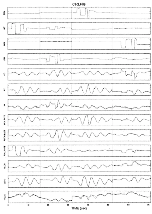
Figure 10 Time history comparison ofmeasured data and the response of the identified model for C10LF69 case ... .40
Figure 11 Time history comparison of measured data and the response of the identified model for D10LA310 case ... .41
Figure 12 Time history comparison of measured data and the response of the identified model for AHF68 case ... .42
Figure 13 Verification of the identified model.. ... .45
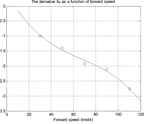
Figure 14 Variation offorward force/velocity derivative Xu with forward speed ... 48
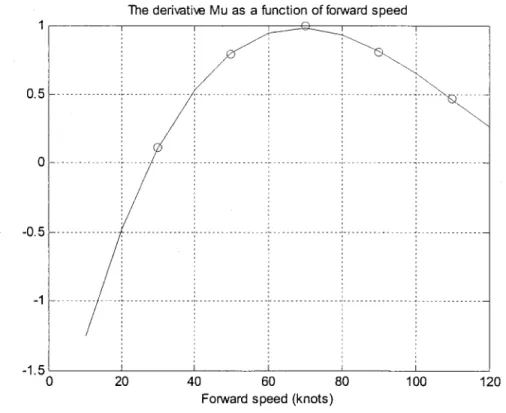
Figure 15 Variation of speed stability derivative Mu with forward speed ... .49
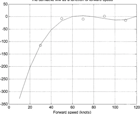
Figure 16 Variation of angle of attack stability derivative Mw with forward speed ... 50
Figure 17 Variation of heave damping derivative Z w with forward speed ... 51
Figure 18 Variation ofpitch damping Mq with forward speed ... 52
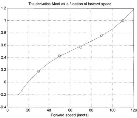
Figure 20 Variation of pitching moment due to collective M col with
forward speed ... 54
Figure 21 Variation of pitching moment M1on due to longitudinal cyclic with forward speed ... 55
Figure 22 Variation of lateral static derivative Lv with forward speed ... 59
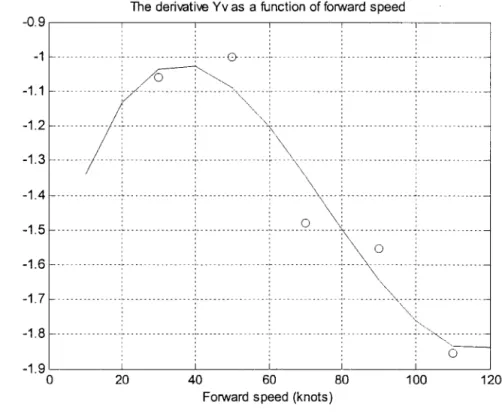
Figure 23 Variation of si de force derivative Yv with forward speed ... 60
Figure 24 Variation of roll damping derivativeLP with forward speed ... 61
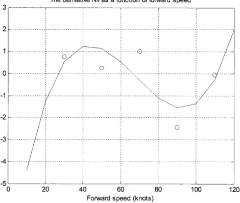
Figure 25 Variation of directional static stability derivative Nv with forward speed ... 62
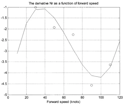
Figure 26 Variation of yaw damping derivative N, with forward speed ... 63
Figure 27 The Top-Level CIFER® software organization ... 67
Figure 28 The lateral stick input (S1a1 ) autospectrum ... 69
Figure 29 The roll rate response (p) auto spectrum to lateral stick input(S1a1) ••••.•••• 69 Figure 30 The roll-rate response (p) to lateral stick input(S1
aJ,
(15 s window) ... 72Figure 31 Composite roll-rate response (p) to lateral stick input ( S1a,) , obtained by a combination of 5 windows (2, 3, 5, 8, 10 s) ... 72
Figure 32 The Bode plot of the pitch rate response to longitudinal input; ( q 1 sion) second arder transfer function fit with flight test data ... 76
Figure 33 The Bode plot of the roll rate response to lateral input; ( p 1 S1a1) first arder trans fer function fit with flight test data ... 77
Figure 34 The Bode plot of the yaw rate response to pedal input; ( r 1 S ped) second arder trans fer function fit with flight test data ... 78
Figure 35 The Bode plot of the normal acceleration response to collective input, ( nz 1 seo/) second arder transfer function fit with flight test data ... 79
Figure 36 The on-axis (pitch rate, q) and off-axis (roll rate, p) responses to longitudinal input (sion ) ... 82
Figure 38 Bode plots comparison between flight data and identified
longitudinal madel frequency response, for w/ 81on •••••••••••.•••.•••••••••••••••...•.• 88
Figure 39 Bode plots comparison between flight data and identified
longitudinal madel frequency response, for q 1 81on •••••••••••••.••.••••••••••••••••..•. 89
Figure 40 Bode plots comparison between flight data and identified
longitudinal madel frequency response, for a x 1 81on •••••••••...••.•.•...•..••••.•••.•• 90
Figure 41 Bode plots comparison between flight data and identified
longitudinal madel frequency response, for u 1 8col ....•.... , ...•..••••••.•.•.•. 91
Figure 42 Bode plots comparison between flight data and identified
longitudinal madel frequency response, for q 1 8col .••.•...••.••..•. 92
Figure 43 Bode plots comparison between flight data and identified
longitudinal madel frequency response, fora x 1 8col ... 93
Figure 44 Bode plots comparison between flight data and identified
longitudinal mo del frequency response, for az 1 8col ...•...• 94
Figure 45 Bode plots comparison between flight data and identified
lateral/directional madel frequency response, for p 1 81a1 •••••••••••••••••••••••••••• 95 Figure 46 Bode plots comparison between flight data and identified
lateral/directional madel frequency response, for r 1 81a1 ••••••••••••••••••••••••••••• 96
Figure 47 Bode plots comparison between flight data and identified
lateral/directional madel frequency response, for a Y 1 81a1 ••••••••••••••••••••••••••• 97 Figure 48 Bode plots comparison between flight data and identified
lateral/directional madel frequency response, for v 1 8ped ... 98
Figure 49 Bode plots comparison between flight data and identified
lateral/directional madel frequency response, for r 1 8ped ... 99
Figure 50 Bode plots comparison between flight data and identified
lateral/directional madel frequency response, for a Y 18 ped ... 1 00
Figure 51 The verification of the longitudinal madel in the LHA37 case ... .101 Figure 52 The verification of the lateral/directional madel in the LHA37 case ... 102 Figure 53 Magnitude, phase and coherence plots of roll attitude (rf;)
as response to lateral stick input (81
aJ,
for HQ analysis ... 104 Figure 54 The least squares fit for the phase delay calcula ti on in HQ analysis ... 1 05Figure 55 Bandwidth-phase delay criteria for roll axis tracking task
according to the standard ADS-33D ... l06 Figure 56 The Newton-Raphson algorithm ... 123
aY Acceleration component along the lateral body axis
az Acceleration component along the normal body axis
b Bias
bw Bandwidth
GM Gain Mar gin (of open loop response)
L Component of the resultant aerodynamic moment about the longitudinal body axis. In derivatives: Derivative of L
L Component of the specifie resultant aerodynamic moment about the longitudinal body axis
LP Roll damping derivative
M Component of the resultant aerodynamic moment about the lateral body axis. In derivatives: Derivative of M
M Component of the specifie resultant aerodynamic moment about the lateral body aXIS
N Component of the resultant aerodynamic moment about the normal body axis. In derivatives: Derivative of N
N Component of the specifie resultant aerodynamic moment about the normal body axis
p Roll rate
s Laplace variable
T Period length
u Component of the air velocity along the longitudinal body axis
v Component of the air velocity along the lateral body axis
X Cornponent of the resultant aerodynarnic force along the longitudinal body axis.
In derivatives: Derivative of
X
X Cornponent of the specifie resultant aerodynarnic force along the longitudinal body axis
Y Cornponent of the resultant aerodynarnic force along the lateral body axis. In derivatives: Derivative of Y
Y Cornponent of the specifie resultant aerodynarnic force along the lateral body aXlS
Z Cornponent of the resultant aerodynarnic force along the normal body axis. In derivatives: Derivative of Z
Z Cornponent of the specifie resultant aerodynarnic force along the normal body aXlS a Angle of attack
fJ
Angle of sideslipr
Coherence functiono
Control deflection 11 Finite variation01a1 Lateral control input Ç Darnping ratio () Pitch angle À Eigenvalue r Tirne delay rjJ Roll angle If/ Y aw angle OJ Angular frequency
=
2 1r fAIAA CIFER CG CZT DFVLR DoF FADEC FFT GPS HQ IC LTI MAP MIMO MISO ML MMLE MTE NASA NRC OAT PlO RPM SI SISO
American Institute of Aeronautics and Astronautics Comprehensive Identification from FrEquency Response Center of Gravity
Chirp-Z transform
German Aerospace Center Degrees of Freedom
Full Authority Digital Engine Control Fast Fourier Transform
Global Positioning System Handling Qualities
Instrumentation Center Linear Time Invariant Maximum a Posteriori
Multiple-Input/Multiple-Output Multiple-Input/Single-Output Maximum Likelihood
Modified Maximum Likelihood Estimation Mission-Task-Element
National American Space Agency National Research Council
Outside Air Temperature Pilot-Induced Oscillations Revolutions Per Minute International Unit System Single-Input/Single-Output
A model is a representation of the essential aspects of an existing system (or a system to be constructed) which presents knowledge ofthat system in a usable form [1].
System identification is an iterative model building process used to obtain an accurate mathematical description from measured system responses [2]. When applied to an aircraft, system identification is a procedure by which a mathematical description of vehicle dynamic behavior is extracted from flight test data (measured aircraft motion).
The field of aircraft stability and control exemplifies a successful application of system identification technology. By identifying stability and control derivatives from flight test data, accurate linear models can be used for control law design or in the estimation of handling qualities parameters. In cases where wind-tunnel data are unavailable or where flight safety into untested regions is of concem, flight-calculated derivatives are extrapolated to predict aircraft behavior prior to flight into these regions. High-fidelity simulators require stability and control data giving an accurate representation of the actual flight vehicle.
Unlike the flight dynamics of most fixed wing aircraft, the dynamics of rotary wing aircraft are characteristically those of a high order system. The large number of degrees of freedom associated with the coupled rotor-body dynamics leads to a large number of unknown parameters to be estimated. Based on previous experience in rotorcraft parameter estimation, it has been agreed that at least a 6 DoF model formulation is necessary to describe helicopter flight dynamics. The coupled, 6 DoF model does not include the high frequency main rotor modes (flapping, lead-lag, twisting), yet it is capable ofmodeling rotorcraft dynamics fairly accurately [3]:
The coordinated approach to rotorcraft system identification is divided into three major parts [2]: a) instrumentation and filters, which covers the entire flight data acquisition process including adequate instrumentation and airbome or ground-based digital recording equipment; b) flight test techniques, which are related to the selected helicopter maneuvering procedures. The input signais have to be optimized in their spectral composition to excite all response modes from which parameters are to be estimated; c) analysis of flight data, which includes the mathematical mode! of the helicopter and an estimation criterion devising a suitable computational algorithm to ad just starting values or a priori estima tes of the unknown parameters un til a set of best parameter estimates that minimizes the response error is obtained.
Motions OPTIMIZED INPUT A PRIORI VALUES Input ROTORCRAFT Actual response Data Analysis Measurements DATA COLLECTION AND COMPATIBILITY IDENTIFICATION CRITERIA Model Response
Figure 1 The basic concept of helicopter system identification
Corresponding to these strongly interdependent topics, four important aspects of system identification have to be carefully treated [2] (Figure 1 ):
b. accurate data gathering of system inputs and outputs involving measurement techniques;
c. mathematical models and the corresponding simulation describing the phenomenon being investigated;
d. estimation methods to extract unknown parameters including model structure determination.
1.1 General description of Bell 427
The Bell 427 is designed as a multiple purpose light helicopter. It is ideally suited for a wide variety of applications including executive and commuter transport, and cargo missions. The Bell 427 has a normal gross weight of 6350 lb and a maximum cruising speed ofup to 135 knots. A three view drawing of the Bell427 is given in Figure 2.
The pilot control inputs are augmented by hydraulic servo actuators. Movement of the cyclic stick is transmitted through the servo actuators to the swash plate, which actuates the rotating controls to the main rotor. A mechanical linkage through the collective servo actuator to the swash plate collective lever transmits movement of the collective control stick. The pedals provide the ability to control the tail rotor thrust in order to compensate for engine torque and to control the directional heading of the helicopter. The hydraulic servo actuator reduces the force required to move the pedals.
Prior to being transmitted to the rotor system, all cyclic and collective movements are transmitted through the mixing bell crank, which is located at the bottom of the control column. The mixing bell crank coordinates control movement so that when blade pitch is changed by moving the collective stick, the cyclic servo actuators and linkage also move in order to keep the swash plate in its relative plane.
The Bell 427 main rotor system uses a soft-in-plane flex bearn type hub with composite main rotor blades. It consists of a single composite yoke, elastomeric dampers and lead-lag/pitch change bearings, metallic pitch homs, grips, and mast and blade attachment components.
36.0 Fr ==~==
,.
1.2FT (.36M) 1 + - - - -42.GFT _ _ _ ···_(_to_.9_8_M_)_·· _ _ _ _ _ _ _ _ _ _ _ ,.. (12.99 M)The four individually replaceable mam rotor blades are constructed of composite materials. Each blade assembly consists of a fiberglass spar, Nomex honeycomb core, fiberglass skins and trailing edge strips, and a leading-edge stainless steel abrasion strip. The design RPM is 395 rot/min with a tip speed of 765 ft/sec (233 mis). Airfoil sections of the blade vary along the span.
The tail rotor is a two bladed teetering pusher type with composite blades, a metallic yoke, and elastomeric flapping bearing. The two tail rotor blades are constructed with fiberglass fabric skins, a unidirectional fiberglass/epoxy spar, and a nomex honeycomb core for corrosion avoidance. The design RPM is 2375 rot/min with a tip speed of 705 ft/sec (215 rn/sec).
The Bell 427 helicopter is powered by two Pratt & Whitney PW207D turbo shaft engines. The engine fuel control system is a single channel Full Authority Digital Electronic Control (F ADEC) with hydro mechanical backup. Each Pratt & Whitney PW207D turbo shaft engine is rated at 710 shp (529 kW) for takeoff (5 minutes), and 625 shp ( 466 kW) for maximum continuous power.
1.2 Optimal input design
Accuracy and reliability of parameter estimations depend on the amount of information available in the aircraft response. A good testing design accounts for practical constraints considered during the flight tests, while minimizing the flight test time [ 4]. The overall goal is the design of an experiment producing data from which model parameters can be accurately estimated. In this way, the system modes are excited so that the sensitivities of the model outputs to the parameters are high and correlations between parameters are low.
The design of an optimal input for accurate model parameter estimation requires high excitation of the system, which is opposite to practical constraints considered in flight-testing. One such practical constraint is the requirement that the output amplitude (e.g., in angle of attack or sideslip angle) variations about the flight test trim condition are limited to ensure the validation of the presumed model structure. Input amplitudes should be constrained for the same reasons, and in addition, to avoid non-linearities such as mechanical stops and rate limiting when the model is linear.
The inputs should excite all the modes of the analyzed model and should minimally excite the un-modeled modes. The system modes are best excited by frequencies near the system natural frequencies. Input frequencies much higher than the system natural frequencies give negligible responses, or excitation of higher frequency un-modeled modes. Very low input frequencies may result in static data.
The first form of multi-step test input signal that is traditionally used for the identification of fixed-wing aircraft is the doublet input. This input excites the short period mode in the longitudinal motion and the Dutch roll in the lateral mode. For a helicopter, although doublet inputs are of limited value, they are capable of exciting the modes in each axis. The doublet inputs are used together with other types of inputs, as they are not ideal for the highly coupled helicopter model.
The second form of multi-step test input signal which is used widely for rotorcraft and aircraft system identification is the "3-2-1-1" band-optimized signal. Figure 3 shows the Power Spectral Density (PSD) of four types of inputs: step, doublet, 3211 signal and a 3211 improved signal, as function of the normalized frequency [2]. Note that the multi-step input signal 3211 was developed by Koehler at Deutsche Forschungs und Versuchsanstalt für Luft und Raumfahrt (DFVLR).
Power Spectral
Density
0 1
Normalized FrequencyϥAt
Figure 3 Frequency spectra oftypical inputs
5
For the Bell 427 Parameter Estimation Program, the aircraft motion is perturbed from trim position by applying a sequence of time-domain control pulses of varying lengths and altemating signs, referred to as 2311 control inputs, where the digits refer to the number of unit time intervals between control reversais (Figure 4). This input is similar to the DFVLR 3211 multi-step input except that in the Bell 427 case the first step is 2 s long and the second step is 3 s long. The length of the unit pulse should be a quarter period of the main response mode [ 5]. The multistep control input was used for separa te excitation of pitch, heave, roll and yaw. Following to 2311 input, the controls are retumed to their nominal trim positions.
The common feature to all acceptable inputs is the presence of step variations represented in Figure 4 in the form of rapid and distinct changes in slopes. Results indicate that as long as these steps are present, relatively simple inputs are very efficient to obtain good estimates of the stability and control derivatives.
••• =t •••••••..
~ ---c--- ____ r::-:<---c: .3 --- --r----0 5 10 15 0 5 10 15 --- ---~--- j,.J---' ' ' ' 0 5 10 15 Time [s] Time [s]Figure 4 Independent 2311 four-axes control inputs for Bell 427
The advantages of the 2311 control input are:
a. sufficiently high frequency content, provided by the altemating input strokes, m order to improve control derivative estimation;
b. ability to excite all the natural aircraft modes; c. short time duration, easy to execute and to repeat;
d. no excitation of the higher frequency rotor modes, which are not included in the 6 DoF model.
Small maneuvers are suited to locally linearized aerodynamic models. Large maneuvers exceed the range of validity of locally linearized models and thus necessitate the use of
aircraft, the range between the lower and upper bounds is large, thus the best maneuver amplitudes are those located near the middle oftheir acceptable maneuver range [6].
The frequency sweep test techniques are recently used in the field of rotorcraft system identification, by Tischler et al. [7]. The frequency bandwidth of interest depends on the test objectives. For helicopter flying qualities studies, the typical frequency range of interest is between 0,5 Hz and 2Hz. In cases where the test objectives include rotor modes identification, the maximum frequency range of interest may be as high as 6 Hz [8]. In the frequency sweep tests, the pilot pro duces a sinusoidal input about a reference trim condition, beginning at very low frequency and progressively increasing the inputs frequency. Thus, the frequency sweep test should contain at !east 3 s of static trim data at the beginning and the end of the record. The total record length should be three to four times the maximum period of interest, i.e. a 60-90 s record length [7]. Figure 5 depicts a typicallateral frequency sweep.
1 0.5 ::::
-..::.0:: 0 .2 "lji c;5 à> -0 5 • 1S _J -1 Tirne {sec)1.3 Flight test instrumentation
The accuracy of the parameter estima tes is directly dependent on the quality of the flight test measured data, and hence, high accuracy measurements ofthe control inputs and of the motion variables are a prerequisite for the successful application of the methods of flight vehicle system identification.
The Bell 427 flight test data for system identification purposes were mainly obtained from the following subsystems:
a. a laser gyro package for the roll, pitch and yaw rates (p, q, r), for the roll and pitch attitude ( rp, B) and for the heading angle (If/) measurements;
b. linear accelerometers installed near the aircraft center of gravity (CG) for the longitudinal, lateral and vertical accelerations measurements (ax, ay, az);
c. potentiometers to measure the pilot control inputs (8Iong, O!at, Oped, Ocoi);
d. a swivel-head air data boom equipped with pressure sensors and vanes for the following measurements: total air speed, angle of attack a and sideslip angle
/3;
the nose boom is mounted in front of the helicopter to avoid main rotor wake interactions;e. a pressure transducer for altitude, rate of climb and airspeed measurements; f. an Outside Air Temperature (QAT) probe for temperature measurements;
g. a flight test computer for the real time helicopter positioning (from Global Positioning System data, GPS) and weight and balance calculations.
In order to avoid larger changes in the helicopter mass and the CG location during the flight, the helicopter was refueled after one hour of flying time. The tests were performed in level flight, moderate and fast climb, moderate descent and fast descent, over a speed range of 30 knots to 110 knots at intervals of 20 knots.
Within one test run, only one control at a time was used to excite the on-axis response of the helicopter and to avoid correlation with other controls. Figure 6 shows sorne typical responses of the helicopter to on-axis input signais.
~bDcrtrl 1~1
0 5 10 15 20 25 0 5 1 0 15 20 25 "i:~---rr,:ft
-- ---\---
---~
l
r
J/'Y.:
~
.:
'
§
--=u---u~--- ~--
-~--- -Tr~~~~---. : Ci : : ' : a:: ' ' 0 10 20 30 0 10 20 30~
b---ryn_: _________
··~---,---1
j
hYl-f\~.~-~L
--.
~
8tw
mmmFmm
~ ~~JmVnmnmmmnmnm
0 5 10 15 20 25 0 5 10 15 20 25~
FrJmnlmmn1mnml.
~ bfV~~
mm
0 5 10 15 20 25 0 5 10 15 20 25 Time [s] Time [s]Figure 6 Characteristic helicopter responses to different inputs
All data needed for the parameter estimation were digitized and recorded on board of the helicopter at a sample rate of 50 samples/sec. During the flight tests, the measured signais were sent by telemetry to the ground station where the time-histories of selected variables were presented on both monitors and strip charts for quick on-line verification.
Real-time data reduction was conducted to isolate data inconsistencies and data transmission errors. By use of these on-line data checks together with pilot's comments it was relatively easy to: a) control the tests; ·b) detect major data errors (e.g. sensor
malfunction, spikes, etc.), data inaccuracies, disturbances (e.g. drifts, large coupling in controls, turbulence, etc.); c) decide if the data point was a "good" one or if it needed to be repeated.
The off-line data processing for system identification purposes included: a. conversion to the same system of units;
b. detection and removal of data dropouts; c. low-pass filtering;
d. corrections for the center of gravity;
e. calculation of additional variables, such as the speed components u, v, w.
Table I and Table II show the sign conventions for the control positions and for the measured response variables.
Table I
Sign conventions used for control positions
Control position Positive sign convention Neutral (zero) convention Longitudinal stick position Cyclic stick moves forward Full aft stick Lateral stick position Cyclic stick moves to the right Fullleft stick Directional pedal position Right pedal moves forward Fullleft pedal
Table II
Positive sign conventions for response variables
Data set Response variable Positive sign convention Angle of attack a AIC nose moves up
Sideslip angle f3 AIC nose moves to the left
Air data True airspeed V Forward
Longitudinal airspeed u Forward
Lateral airspeed v Right
Vertical airspeed w Upward
Longitudinal acceleration a Forward
Linear x
Lateral acceleration a Y To the right
accelerations
Vertical acceleration a z Downward
Bank angle (roll angle) tjJ Helicopter tums clockwise about
roll axis as seen from rear Attitude
Pitch angle fJ AIC nose moves up angles
Helicopter tums clockwise about Y aw angle 1f1
yaw axis as seen from above Roll rate p Helicopter tums clockwise about
roll axis as seen from rear Angular
Pitch rate q AIC nose moves up rates
Yaw rate r Helicopter tums clockwise about
yaw axis as seen from above
Sorne of the helicopter motion measurements were very noisy, thus, a low-pass filtering was applied on these data measurements. Analog filters reduce the high frequency amplitudes and influence the phase characteristics of the measured signal. For example, in the case of high order filters, the phase shifts may be significant at frequencies far below the filter eut-off frequency. The identification is based on the amplitude and phase relationship between the individual measurements, and for this reason, filters may deteriorate identification results. Zero-phase shift digital filters were applied in order to eliminate the unwanted higher frequency effects and noise and to reduce the sampling rate.
Most of the quantities of interest ( displacements, speeds and accelerations) are referred to helicopter body axes, as shown in Figure 7. The origin of the body-axes system is at the CG. The entire axis system moves and rotates with the helicopter. The x-axis is always parallel to the fuselage reference line and in case where the CG is in the plane of symmetry, both the x and z-axes are in the aircraft's symmetrical plane. The y-axis is normal to the plane of symmetry.
In Figure 7, X, Y, Z are the forces, L, M, N are the moments, u, v, w are the linear speeds, andp, q, rare the angular rates. The aircraft attitude with respect to the inertial system is defined by the three Euler angles If (heading angle), B (pitch attitude), and rjJ (roll attitude). The body-axis helicopter angular rates (p, q, r) are defined as projections of the angular velocity vector (with respect to the inertial system of coordinates) on the body axes [9].
The roll rate p, pitch rate q, and yaw rater are the components of the angular velocity in the body-axis system of coordinates, ~ ,
è,
and lj! :p
=
~ -lj! sineq
=
è
cos rjJ+
lj! cose
sin rjJr
=
lj! cos ecos rjJ -è
sin rjJ(1.1)
The angle of attack (a ) and angle of sideslip ( f3) vanes measure the local flow direction. The effects of flow components resulting from angular velocities and flight path curvature introduce errors in the measured flow angles with respect to the true angle of attack or the sideslip angle [ 1 0].
In order to use the angle of attack a in the true airspeed measurement point, it has to be changed from the CG point to the instrumentation centre (IC) of true airspeed:
aie
=
acG-x~
(azcG-gcosBcosr/J)- xa qv
v
(1.2)where x a is the distance (along the x axis direction) between the a vane and the aircraft
CG, Vis the true airspeed, azcG is the normal acceleration at the CG and q is the pitch rate.
In order to correct the sideslip angle measured at IC with respect to CG, by taking into consideration the yaw rate r and roll rate p effects, the expression of the sideslip angle is written as follows:
Xp Zp
f3Ic
=
f3cG + - r - - pv
v
(1.3)where xfJ is the distance (along the x axis direction) and zfJ is the distance (along the z
axis direction) between the f3 vane and the aircraft CG and p and r are the roll rate and the yaw rate, respectively.
The sideslip vane measures the flank angle of attack,
a
1, as defined by Figure 8:-1 v
a1
=tan-u
The real sideslip angle, fl1c, at the IC is further expressed from Figure 8 as follows:
---===~ 1 1 1 - - - / 1 / / 1
---
/ 1 J -- -- -- -- -- 1 / / 1 Uic / 1 1 a - - - )- :.JC. _ _ _ _ _ / / / /"" / / 1 / / / / / - - 1 / ---~~Figure 8 The correction of sideslip angle fl
1 1
(1.4)
(1.5)
The longitudinal, lateral and normal speed components at the sensor position (IC) are calculated as functions of the true airspeed, angle of attack and angle of sideslip at the IC:
u1c =V cosa1c cos fl1c
v1c
=
Vsinfl1cW 1c
=
V sin a IC COS fl1cThe true airspeed at IC is written as a function of the V at CG:
v;c
=
VCG +wxr
Using Equation (1.7) the true airspeed at CG is expressed as:
fcG
=
vic - w xr
(1.6)
(1.7)
The vector product between angular velocity, w , and the position vector,
r,
is written as follows: i j k w xr=
p q r =z(qz-ry)+ ](rx- pz)+k(py-qx) x y z (1.9)The speed components at the CG are obtained by replacing Equation (1.9) in Equation (1.8), as follows:
Ucc =uic -qz+ry Vcc = v1c -rx+ pz Wcc
=
WIC-py+qXThe true airspeed at the CG, Vcc, results from the following equation:
where ucc, V cc, Wcc, are given by Equation (1.10).
(1.10)
(1.11)
The distance between the sensor position and the helicopter CG affects the measurements of linear accelerations because the measured signais will contain acceleration components due to the helicopter angular motion.
The accelerations can be obtained by differentiation of the speed given by Equation (1.8):
(1.12) But, since
r=wxr (1.13)
Equation (1.12) can be written in the following form:
(1.14) The airframe is considered rigid thus,
y
=x
= :i = 0 ; using this, the linear accelerations at the CG (axee, a ycc, a zee) are written in full y expanded formas follows:axCG
=
ax/C+
x(q2+
r 2) -y(pq-f )-z(pr +
q)
ayCG
=
ay!C+
y(r2+
p2 ) -z(qr-jJ )-x(qp +f)
azCG
=
aziC+
z(p2+
q2
) -x(rp-
q )-
y(rq +jJ)
( 1.15)
Equations (1.15) show that the rotational accelerations (
p,q,r)
are needed to correct the linear acceleration measurements at the CG. Because no measurements were available, the differentiated rates were used.1.4 Model structure
The choice of a model structure is a critical step in system identification, which might affect both the degree of difficulty in extracting the unknown parameters, and the utility of the identified model in its intended application. Simple decoupled models characterizing the helicopter dynamics over a limited frequency range are suitable for handling qualities applications, while coupled 6 DoF models covering a broader frequency range are needed for simulator applications. In the case of advanced high bandwidth rotorcraft flight control system design, these models should consider the coupled fuselage/rotor/air mass dynamics. The best choice is the simplest model structure that serves the intended application [3].
Model structures can be broadly divided into two groups: nonparametric and parametric [ 11]. A nonparametric model is one in which no model order or form of the differentiai equations of motion is assumed. Nonparametric models are expressed as frequency responses between key input/output variable pairs ( e.g. pitch-rate response to longitudinal stick) which are calculated using Fast Fourier Transform techniques. Nonparametric models are presented in Bode plot format of Log-magnitude and phase of the input-to-output transfer function versus frequency. Typical applications of nonparametric identification results are handling-qualities analyses based on bandwidth
The parametric model requires the assumption of both system order and the structure of the system's dynamical equations. The simplest parametric model structure is a transfer function, which is a pole-zero representation of the input-to-output relationship; these parametric models have relatively few unknown parameters. A more complex parametric model is a full 6 DoF (or higher) set of coupled linear differentiai multi-input/multi-output (MIMO) state-space equations, derived from Newton's laws applied to the helicopter model. Common applications of parametric models include control system design, wind-tunnel model validation, and mathematical model derivation and validation.
The adopted model for this study was a fully coupled, 6 DoF state space model [12]. Ali higher degrees of freedom, associated with the rotor, power plant/transmission, control system and the disturbed airflow, were embodied in a quasi-steady manner in the equations of motion, and have lost their own individual dynamics and independence as degrees of freedom in the mo del reduction.
The basic flight dynamics equations are the linear momentum and angular momentum equations: - d ( -) F=-mV dt (1.16) - d (-) M=-H dt (1.17)
where F is the extemal applied force, M is the extemal applied moment about the center of gravity, Vis the true airspeed vector, and H is the angular momentum vector about the center of gravity. Equations (1.16) and (1.17) need to be referred to the rotating aircraft body-system.
If OJ is the angular velocity vector of the body axis system with respect to the inertial
coordinates system, the rules for transforming vector derivatives into the rotating aircraft body system give the following equations:
F
=~(mV)+w
x(mv)dt
- d (-)
-M=-H+wxH dt
The angular momentum is further given by:
(1.18)
(1.19)
(1.20)
The matrix in Equation (1.20) is the inertia tensor expressed in the body fixed system of coordinates. The components of OJ in the body axis system of coordinates are p, q and r.
The components of V in the body axis system of coordinates are u, v and w. The indices from the CG components ofvelocity ucG, V cG and WcG are dropped, for brevity.
For aircraft stability and control applications the time derivatives of the mass and of the inertia tensor are neglected. To avoid larger changes in mass and CG location the helicopter was refueled after a total flying time of about one hour.
Equations (1.18) and (1.19) can further be written in the following scalar form: - Forces equations:
Fx =
m(u
-rv+qw)FY
=rn(
v+
ru- pw)
Fz
=
m(w+ pv-qu)- Moments equations:
L
=
pfx -qfxy -rfxz +qr(Iz -Jy)+(r2 -q2)Jyz- pqfxz +rpfxy M =-pfxy +qfy -flyz +rp(Ix -IJ+(p2 -r2)Jxz -qrfxy + pqfyz N=
-pfxz -qfyz +flz + pq(IY -fJ+(q2 - p2)fxy -rpfyz +qrfxz(1.22)
where Fx , FY and Fz are the components of the extemal applied forces, and L, M and N are the components of the extemal applied moments.
The aircraft mass distribution is considered symmetrical relative to the xz-body plane of symmetry. Renee, the moments of inertial xy
=
0 and/yz=
0 and the general moments ofinertia expressions given by Equations (1.22) become:
Jxp =(!Y- !Jqr + J zx(f+ pq) + L IA =(Iz -!Jrp+fzx(r2 -p2)+M
!zr= (Ix- Iy)pq + Izx(P- qr) + N
(1.23)
Expressing Fx , FY and Fz as functions of the aerodynamic forces X, Y and Z, and the gravity force, as follows:
Fx =X -mgsinB FY =Y +mgcosBsinrp Fz
=
Z +mgcosBcosrpand introducing the forces given by Equations (1.21) into Equations (1.24) gives:
mu =m(vr-wq)+X -mgsinB
mv
=
m(wp -ur)+ Y+ mgcosBsinç6 mw= m(uq- vp) + Z +mg cosBcosç6(1.24)
(1.25)
The kinematic equations for Euler rates are obtained from Equation (1.1) as follows:
~
=
p + q sin ç6 tane
+ r cos ç6 tane
e
=
q cos ç6 - r sin ç6 . sin ç6 cos ç6If/= q + r
-cosB cosB
Equations (1.23), (1.25) and (1.26) are nonlinear because of the gravitational and rotation related terms in the force Equations (1.25) and the appearance of products of angular rates in the moment Equations (1.23).
Using small perturbation theory, the products of angular rates are assumed to be small and therefore, can be neglected in the moment Equations (1.23). Renee, a simplified set of equations results:
L=IxjJ-Ij·
M=l/J (1.27)
Furthermore, by dividing the force Equations (1.25) by the mass, rn, and multiplying the simplified moment Equations (1.27) by the inverse inertia matrix, forces and moments are presented as "specifie" quantities:
Specifie forces: X=XIm Y=Yim (1.28) Z=Zim Specifie moments: (1.29)
Then, using the specifie forces (1.28) into Equations (1.25) and the specifie moments (1.29) into Equations (1.23) the following two sets of equations are obtained:
the linear accelerations:
the angular accelerations:
p=L
q=M
(1.31)In 6 DoF form, the motion states are usually arranged in the state vector as longitudinal
(u, w,q,B) and lateral (v,p,rjJ,r,l!f) motion subsets, as follows:
x= [u, w,q,B, v,p,rjJ,r,l!f
Y
(1.32)where u, v and w are the translational velocities, p, q and r are the angular velocities along the body-axes and rjJ , B and '!/ are the Euler angles, defining the orientation of the body axes relative to the earth.
The control vector has four components: longitudinal cyclic,
o
1on, lateral cyclic,o
1a1 , tailrotor collective (pedals), oped' and main rotor collective, ocol:
(1.33)
In the small perturbation theory, the helicopter's behavior can be described as a perturbation ~X from its trim position Xe, and is written un der the following form:
(1.34) Taylor' s theo rem for analytic functions implies that if the force and moment functions and all their derivatives are known at the trim point, then the behavior of that function anywhere in its analytic range can be estimated from an expansion of the function in a series about the trim point.
The forces and moments arise from aerodynamic, gravitational and control effects. The series of Taylor expansion for the aerodynamic force on x-axis, X, pro vides [ 12]: