Anisosphere analysis of the equivalence between a precessing Foucault pendulum and a torsional balance

(1)

Content from this work may be used under the terms of theCreative Commons Attribution 3.0 licence. Any further distribution of this work must maintain attribution to the author(s) and the title of the work, journal citation and DOI.

Published under licence by IOP Publishing Ltd

International Conference on Mathematical Modelling in Physical Sciences IOP Conf. Series: Journal of Physics: Conf. Series 1141 (2018) 012064

IOP Publishing doi:10.1088/1742-6596/1141/1/012064

Anisosphere analysis of the equivalence between a

precessing Foucault pendulum and a torsional balance

R Verreault1

Université du Québec à Chicoutimi,

555, boulevard de l’Université, Saguenay, Québec, Canada G7H 2B1. E-mail: rverreau@uqac.ca

Abstract. The residual anisotropy of a real Foucault pendulum is responsible for an oscillatory behaviour of the precession angle according to the original description given by Kamerlingh Onnes in his dissertation. A simulation of the experimental procedure of enchained runs, consisting of starting a short experiment at the azimuth at which a precedent similar experiment has been stopped, has been performed using the anisosphere model. It leads to the conclusion that the precessing pendulum undergoes oscillations in precession associated with an extremely shallow potential well analogous to the potential well of a very slow torsional balance. Such systems are therefore rendered sensitive to extremely-low-energy perturbations. To the author’s knowledge, the hypersensitivity of the oscillatory precession of the anisotropic Foucault pendulum has been unravelled for the first time thanks to the analysis and visualization power of the anisosphere model. In particular, the periodic apparent motion of celestial bodies appears to modify the anisotropy characteristic of the precession potential well. This may provide likelihood for the similar responses of the paraconical pendulum of Allais during the 1950’s and of the torsion pendulum of Saxl and Allen in 1970 to certain Sun-Moon-Earth syzygies.

1. Introduction

From 1954 to 1960, Maurice Allais conducted a series of very well planned 30-day long continuous experiments, day and night, with a new type of Foucault pendulum designed by him for that purpose. Instead of the original wire-in-chuck suspension of Foucault, Allais opted for a short rigid compound pendulum solidary of a steel ball rolling on a flat steel plate [1], a system that he christened paraconical pendulum, apparently because, contrary to the ideal conical pendulum which has a truly spherical potential well, that one strictly possesses a rotation symmetric trochoidal potential well, insofar as it is perfectly isotropic. On the other hand, Allais made his pendulum anisotropic by design, using, for most of his experiments, a vertical bronze disk as bob. Hence, the moment of inertia and, consequently, the period of oscillation were maximal for oscillations simultaneously normal to the fixing beam and in the plane of the disk.

In 1879, under the incentive of Kirchhoff, Heike Kamerlingh Onnes (KO, here after) addressed the problem of the anisotropy of Foucault pendulums in his dissertation [2], in order to shed light on the causes of the unwanted elliptical orbits arising after a few minutes in practically every Foucault pendulum implementation. KO defined the amount of linear anisotropy of a pendulum as the rate of phase change 𝛿̇ between the components of a planar (rectilinear) oscillation along the azimuths of shortest (fast eigneaxis X) and longest (slow eigenaxis Y) swinging period

𝛿̇ = 𝜔_𝑋− 𝜔_𝑌 = 𝜔̅(𝐼𝑌 − 𝐼𝑋)

2𝐼̅ . (1)

1

(2)

𝜔𝑋, 𝜔𝑌, 𝜔̅ are the swinging angular frequencies for rectilinear oscillations along X, along Y and

their average respectively.

𝐼_𝑋, 𝐼_𝑌, 𝐼̅ are the swinging moments of inertia for rectilinear oscillations along X, along Y and their average respectively, i.e. for rotations about horizontal axes respectively normal to X, to Y.

KO showed that for small amplitudes (linear oscillator approximation) the pendulum behaviour is governed by the relative amount of linear anisotropy compared to the amount of circular (Foucault) anisotropy 𝜔_𝑅 −𝜔_𝐿, where 𝜔_𝑅 is the angular velocity of a clockwise (right handed) circular orbit, and 𝜔_𝐿 is the angular velocity of a counter clockwise (left handed) circular orbit. In particular, if 𝜔_𝑋− 𝜔_𝑌 > 𝜔_𝑅 −𝜔_𝐿, there are situations where the precession of the swinging azimuth no longer runs through a 360 cycle, but oscillates back and forth about one of the fast or slow eigneaxes, while the ellipticity attains extremal values when the swing azimuth crosses one of the fast or slow eigenaxes. Here, the ellipticity of an elliptical orbit is understood to be the ratio of semi-minor axis to semi-major axis 𝑏/𝑎.

It has also been shown by this author [3,4] with the help of the anisosphere model (see also appendix A1 below) that, for large swing amplitudes, a consequence of the Airy effect is not only the appearance of a significant precession rate as soon as an elliptical orbit builds up, but also a drastic collapse of the phase curve onto the anisosphere equator. This means that the ellipticity becomes quickly saturated to very low minor-to-major axis ratios (< 0.005) in the case of nonlinear pendulums like Allais’ paraconical one. It must therefore be kept in mind that the above considerations are essential to a correct understanding of Allais’ experiments.

Obviously, Allais had recognized those features of his pendulum. Instead of striving at measuring minor axes well in the sub-millimeter domain, he recorded what he assumed to be the Airy precession rate proportional to a minor axis that he did not bother to measure. He also recognized the tendency of strongly anisotropic pendulums to oscillate in precession about an eigenaxis of linear anisotropy (KO effect). Such an oscillatory behaviour in precession implies the existence of a restoring torque in precession and of a corresponding paraboloidal potential well for the swinging azimuth. In fact, he wrote the second order differential equations of that alternating precessing motion and he evaluated its pertinent restoring torque.

Finally, if Allais had tried to measure the azimuth of the minimum of the precession potential well, hence the actual azimuth of that eigenaxis of linear anisotropy, by taking the average azimuth of a large number of oscillations in precession, many hours per run would have been necessary. But the large amplitudes used (0.11 rad) and the important damping encountered would have been prohibitive. Most probably, a single complete cycle of precession would have not been achievable in practice. Allais’ approach has rather been to perform a month-long series of enchained short 14-minute runs restarted every 20 14-minutes in the same azimuth as the end azimuth of the previous run. This ingenious procedure makes the pendulum equivalent to an azimuth measuring instrument featuring supercritical damping at a time constant of the order of one hour. Thanks to that procedure, the paraconical pendulum tracks down the azimuth of the eigenaxis of linear anisotropy on a continuous basis. In this way, any wandering of the eigenaxis azimuth during the day or over many days, for whatever reasons, can be monitored by the pendulum via the evolution of the starting azimuth prescribed from each preceding run.

In the present article, the anisotropy characteristics of Allais’ paraconical pendulum have been modelled on the anisosphere. It has therefore been possible to simulate a typical experiment conducted by Allais. Each simulated 14-minute run is subject to the Foucault effect and to the Airy effect. A novel precession contribution not identified by Allais has been introduced into the model. It stems from spin-orbit coupling and proved necessary to reproduce Allais’ measurements. Allais did not need to bother with that contribution simply because he apparently overestimated the Airy effect.

2. Modelling one of Allais’ experiments

Allais’ book contains many dozen graphs of processed data but very few raw data that would lend themselves to simulation. Such an exception is met with graph IV, page 95 [5]. That example involves a pendulum with smaller anisotropy than in most subsequent experiments, since the bob in that particular case consisted of a lead sphere instead of the usual vertical disk. The important characteristics of the pendulum that have been integrated into the anisosphere model are listed in

(3)

table 1. In particular, with the amount of linear anisotropy being smaller than twice the Foucault in absolute values (𝛿̇ < 2|𝜓̇_𝐹|), such a pendulum at very low amplitudes of the order of 0.0001 rad should behave like a normal KO pendulum, namely develop moderate ellipses but precess monotonically in the cw sense, for the latitude of Paris. However, the operating amplitude of 0.105 rad changes things drastically. Since the azimuths are counted positive in the ccw sense, figure 1 shows that, for experiments started at azimuths on the high side of the slow eigenaxis, cw ellipses develop readily and Airy precession in the same sense as Foucault precession sets in, thus accelerating the evolution towards the slow axis. On the contrary, for experiments started at azimuths on the low side of the slow eigenaxis, ccw ellipses develop and the Airy precession is in the opposite sense to the Foucault precession. Foucault precession is completely compensated after approximately 6 to 8 minutes while Airy precession keeps increasing with increasing ellipticity. At the end of a 14-minute run, if the initial azimuth is farther away from the slow eigenaxis than ~7 degrees, the final azimuth of that run will lie closer to the eigenaxis than the initial one. In the scheme of enchained runs, such a situation commands that the next run will be started closer to the eigenaxis than the previous one. If, on the other hand, the initial azimuth lies closer to the slow eigenaxis than ~6 degrees, the ccw ellipses grow less rapidly, together with the associated Airy precession. Then Foucault precession is less rapidly compensated, and the final azimuth lies farther away from the eigenaxis than the initial one. That situation commands that the next run will be started farther away from the eigenaxis than the previous one. It can thus be concluded that the experimental procedure of enchained runs results in a stabilisation of the pendulum launch azimuth somewhere on the side of the slow axis azimuth toward which Foucault precession is directed.

The last phase curve on figure 1 (run 24) is essentially an asymptote, at an initial and final longitude of −13.7. This means that the pendulum start-stop azimuth has found a stable equilibrium at 6.85 below the slow eigenaxis azimuth, in full accordance with the above reasoning. In fact, figure 2 shows that, from run to run, the evolution of the launch azimuth is subject to an exact exponential decay toward an asymptotic value. For launches above the slow axis azimuth (runs 0-8), both Foucault precession and Airy precession act in the same sense.

Table 1. Characteristics of Allais’ pendulum that have implemented in the anisosphere

model

Period Foucault rate 𝜓̇𝐹 Anisotropy _{amount 𝛿̇} Amplitude Damping time _constant _{increment Δ𝑡}Integration

s rad/s rad/s rad h:min s

1.826 -0.000055 0.000043 0.105 1:10 15

Figure 1. Simulation of the enchained-runs procedure on the anisosphere. A selection of phase

curves of the 25 runs of this simulated experiment is shown. The experiment is started at an azimuth 45 higher than the slow axis azimuth due to suspension anisotropy, here taken as the origin of longitudes on the anisosphere. As a result of the important Airy effect, the quasi totality of the phase curves are squeezed within a ±1 range about the anisosphere equator. Note that for the sake of graph clarity, the latitude scale has been exaggerated by a factor 10. The last phase curves, not shown, pile up on the asymptotic curve exemplified by run 24, where the final and initial azimuths coincide.

(4)

Figure 2. Damping characteristics of the

enchained-runs procedure. For a pendulum launch at a higher azimuth than the slow eigenazimuth, the consecutive launch azimuths undergo exponential decay toward the asymptotic azimuth 𝜓∞+ = −18 with a

time constant of 6.85 14-min runs. Once the eigenazimuth has been crossed (from run 9on in figure 1), a new asymptote 𝜓∞−= −6.85

prevails, with a time constant of 5.73 14-min runs.

Figure 3. Evolution of the semi-minor axis

for Allais’ experiment (lower blue curve, adapted from [1]) and for the anisosphere model (upper red curve). An important feature reproduced by the model is the tendency toward saturation.

The sequence of runs heads then toward the asymptotic longitude 2𝜓_∞= −36. However, for launches below the slow axis azimuth (runs 9-24), Airy precession and Foucault precession act against each other. A new regime sets in where the asymptotic longitude is now 2𝜓_∞ = −13.7.

Figure 2 indicates that the number of enchained runs necessary to reach the equilibrium azimuth correspond to an overdamped process strictly described by an exponential decay of the azimuth difference between start azimuth 𝜓0 and equilibrium azimuth 𝜓24 (in general 𝜓∞).

Speaking of pendulum swing azimuth instead of anisosphere longitude, for a pendulum launch at a higher azimuth than the slow eigenazimuth, the decay process aims to the asymptotic azimuth 𝜓_∞+= −18 with a time constant of 6.85 14-min runs. Once the slow eigenazimuth has been crossed, the runs on the negative side of the slow axis (from run 9 on) aim to a new azimuthal asymptote 𝜓_∞−= −6.85 with a time constant of 5.73 14-min runs.

Another interesting result of the anisosphere model (figure 3) is the tendency of the minor axis to saturate at a very low value. This is consistent with the characteristic feature of Airy precession according to which the phase curve becomes squeezed against the anisosphere equator, as shown in reference 3. Let us recall [3,4] that the latitude on the anisosphere is 2𝜒 = 2 tan−1_{(𝑏/𝑎) . The}

semi-minor axis b must saturate when the phase curve crosses the slow axis azimuth. Allais’ experimental plot of the minor axis averaged over 1080 individual runs is also reproduced in figure 3 for comparison. As mentioned in the introduction, precession from spin-orbit coupling must be added to Airy precession in order that the model (upper curve in red) would reproduce reasonably well all the features of the experimental curve (in blue) during the runs near the asymptotic situation.

3. A triply-enchained-runs experiment

At some occasions, in order to eliminate certain types of error, Allais decided to conduct experiments with doubly- or triply-enchained runs. Although none of his original measuring data is available, it has been possible in one case to extract the data from the dot positions in the graph

(5)

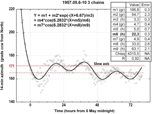
Figure 4. Spectral analysis of a triply-enchained-runs experiment over 3.5 days. The individual

dots represent all the stop-start azimuths connecting the enchained runs. Note that the azimuth units are grads counted positive in the ccw sense. A theoretical function in the form of the sum of a decreasing exponential and of two sinusoidal components is fitted to the data. The known slow eigenaxis from suspension anisotropy is at 171 gr. The steady state equilibrium azimuth (red dotted line) falls 5.7 gr (5.13) below the slow eigenazimuth. Considering 1 run/h in each chain, the damping time constant (m3 in the inset table) is 3.3 14-min runs.

and to perform a spectral analysis on that data with the KaleidaGraph software. The essential features described in the preceding section can be observed, as shown in figure 4. Note that in that graph, the azimuth units are grads instead of degrees (1 gr = 0.9). The known slow axis azimuth from suspension geometry is 171 gr. This triply-enchained experiment (1 run/h in each chain) is started with a first launch at the azimuth 220 gr (essentially 45 above the slow axis azimuth).

One essential difference between this experiment and the one modelled in section 2 is the use of a vertical disk instead of the lead sphere. The linear anisotropy amount is then substantially higher. The consequences are a shorter KO cycle described at higher velocity, a more rapid development of elliptical orbits and a larger Airy precession rate during a 14-min run. One can thus expect, on the higher azimuth side of the slow axis, a faster descent toward the asymptote, and on the lower azimuth side, an equilibrium azimuth closer to the slow eigenaxis, since the excess of Airy precession over Foucault precession yields a greater tendency to bring the final azimuth back toward the slow axis.

All those features are actually observed in figure 4. The total precession angle of run 0 is −11 gr (−10), as compared to −6.5 (1/2 of the longitude change) in figure 1. Considering −2.6 of Foucault precession over 14 minutes in Paris, the amount of Airy/spin-orbit precession in the first 14-min run of this experiment is −7.4, compared to −3.9 in the experiment of figure 1. This faster descent is also corroborated by the shorter time constant of 3.3 runs instead of 6.85 runs in figure 2. Moreover, on the lower side of the slow-axis azimuth, the asymptote is 5.13 below the slow axis, compared to 6.85 in figure 1. In conclusion, the anisosphere simulation is in complete agreement with the transient part of the spectral analysis of that experiment.

(6)

4. Precessing and torsional pendulum equivalence

The anisosphere model has enabled a re-analysis of two typical experiments performed with Allais’ paraconical pendulum during the 1950 decade. It demonstrates without any doubt that an anisotropic pendulum operated according to the procedure of enchained runs, and at amplitudes large enough to generate Airy precession, involves a restoring torque in precession which, were it not for the simultaneous presence of Foucault precession, acts toward the azimuth of longest swinging period (slow eigenaxis). From the existence of a restoring torque in precession, it can be argued that a precession potential well exists with a minimum at the slow eigneaxis azimuth. When operating the pendulum somewhere else than at the Earth equator, the effect of one-way Foucault precession is equivalent to a tilt of that potential well in the same sense as Foucault precession. Consequently, the potential well minimum is displaced a few degrees in the direction of Foucault precession.

Modelling the procedure of enchained runs with the anisosphere shows that the anisotropic pendulum behaves like a faithful azimuth measuring instrument which tracks the azimuth of the minimum of precession potential energy with supercritical damping and with a time constant of a few 14-minute runs. In terms of experiment time, that time constant is of the order of one or two hours. Put in other words, the above statement could read:

the anisotropic pendulum tracks faithfully

the azimuth of the actual minimum of a precession potential well with a 1 to 2 h time constant,

except for a constant offset of a few degrees due to Foucault precession.

The examples presented in sections 2 and 3 confirm experimentally that statement. If, instead of the enchained-runs procedure, an experiment could be pursued continuously for many hours, the restoring torque in precession would allow the swing azimuth to oscillate back and forth about the slow eigenaxis with a precession period of the order of 10 hours (KO period). This means that, contrary to the gravitational potential well governing the swinging pendulum motion with a period of a few seconds,

the precession potential well of an anisotropic Foucault pendulum is extremely shallow and can be perturbed by extremely small energy amounts.

As mentioned in the abstract, one could then associate the precessing anisotropic pendulum to a torsion pendulum with an extremely long angular period. It is reasonable to conceive that such low-energy oscillators could resonate with periodic phenomena whose periods lie in the range of tens of hours and, consequently, prove hypersensitive in detecting such phenomena. It is therefore not surprising if Allais with his paraconical pendulum and Saxl and Allen [6] with their torsional balance have both reported perturbations associated with the alignment of celestial bodies during solar eclipses.

5. The states of a 14-min run as bound states attached to a mobile slow axis

Under those circumstances, after the first six hours of transient response in the experiment of figure 4 have passed, the slow wavy character of the 3-day long steady state response must be attributed to real periodical variations of the azimuth of minimum potential energy with amplitudes of approximately 4.5 (parameters m4 and m7 in the inset) and with the respective periods around 22 h and 63 h (parameters m6 and m9). Of course, nothing can be said at this stage about the nature and origin of those variations in linear anisotropy. However, the anisosphere model can be useful in describing the quantitative features in amount and direction of such anisotropy contributions.

Incidentally, in many of the month-long continuous experiments performed by Allais, some periodicities in precession with statistically significant amplitudes were observed at the precise lunar-day period, as opposed to the solar-day period. In figure 5, the effect of a cyclic perturbing source of linear anisotropy is modelled on the anisosphere.

(7)

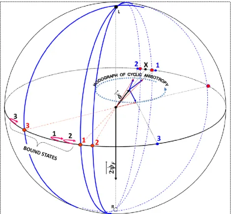
Figure 5. Anisosphere analysis of the influence of a perturbing

slowly varying cyclic linear anisotropy contribution. The result is a cyclic wandering of the linear anisotropy slow eigenaxis. The phase curve of a 14-min run always starts and stops at about 4 to 6 on the low-azimuth side of the slow eigenaxis. It tracks the wandering of the slow eigenaxis with an offset but with very little lag, occupying a set of bound states linked to the slow eigenaxis.

The usual Foucault circular anisotropy vector 2𝜓⃗⃗⃗⃗⃗⃗⃗⃗ (in black) is placed on the polar axis, _𝐹̇ pointing downwards to the cw fast circular eigenstate R and the usual suspension anisotropy fixed vector 𝛿̇ (also in black) lies in the anisosphere equatorial plane, pointing to the fast linear eigenstate X. In the equatorial plane lies also a slowly rotating perturbing linear anisotropy vector (in blue) attached to the extremity of 𝛿̇ . Three different positions of that perturbing vector are shown pointing to the labels 1, 2 and 3 (in blue) along the equator. The vector sums of the fixed and the mobile linear anisotropy vectors (in red) point toward their respective fast linear eigenstates (red points on the equator behind the anisosphere). Their corresponding slow eigenstates are represented by the equatorial red dots on the front side of the anisosphere (labelled 1, 2, 3 in red). The hodograph of the rotating vector lies in the equatorial plane, as would any vector of linear anisotropy. It has been given the shape of a circle for simplicity, but it may have any shape, closed or spiralling, depending on the time dependence of the vector’s module.

The precession events and phase curve evolution happening during one 14-min run can be described as follows. The (blue) meridian planes attached to the respective fast and slow linear anisotropy eigenstates (red dots) contain the characteristic elliptic eigenaxis MN (not shown) which represent the total anisotropy (circular + linear) character of the pendulum. In accordance with figure A4 of the appendix, state N initially in the upper hemisphere acts as the centre of curvature of the phase curves (shown in red and labelled 1, 2, 3 in black). Right after the first minute, ccw Airy precession builds up due to appearance of ccw ellipses, since the phase curves enter the upper hemisphere. The Airy precession rate is represented by a polar vector (not shown) attached to the end of the polar Foucault anisotropy vector, but it points upwards, gradually

(8)

compensating the Foucault precession rate vector. After ~7 minutes, the Foucault precession rate has been completely compensated: circular anisotropy becomes then momentarily zero and the total anisotropy eigenaxis MN lies momentarily in the equatorial plane. At that stage, both of the elliptic eigenstates M and N are swapping their hemisphere, while remaining in their original meridian plane. For the second half of the phase curve, the centre of curvature N lies now way down on its meridian near the lower pole R. The run is then aborted after 14 minutes. At the end, the Airy precession rate vector has grown to about twice the amount of the Foucault precession rate vector, and the extremity of their vector sum ends up on the polar axis somewhere near the upper pole L.

In the steady state situation, as a result of the above state of affairs, the phase curve of a 14-min run always starts and stops at about 4 to 6 on the low-azimuth side of the slow eigenaxis. It tracks the wandering of the slow eigenaxis with very little lag, occupying a set of bound states linked to that eigenaxis.

6. Conclusion

Moddelling the anisotropic Foucault pendulum on the anisosphere allows one to thoroughly study and visualize the complicated behaviour of that instrument, despite the apparent simplicity of its construction and its operation. The residual anisotropy of a real Foucault pendulum is responsible for an oscillatory behaviour of the precession angle according to the original description given by Kamerlingh Onnes in his dissertation. A simulation of the experimental procedure of enchained runs, consisting of starting a short experiment at the azimuth at which a precedent similar experiment has been stopped, has been performed using the anisosphere model. It leads to the conclusion that the precessing pendulum undergoes oscillations in precession associated with an extremely shallow potential well analogous to the potential well of a very slow torsional balance. Such systems are therefore rendered sensitive to extremely-low-energy perturbations. To the author’s knowledge, the hypersensitivity of the oscillatory precession of the anisotropic Foucault pendulum has been unravelled for the first time thanks to the analysis and visualization power of the anisosphere model. In particular, the periodic apparent motion of celestial bodies appears to modify the anisotropy characteristic of the precession potential well. This may provide likelihood for the similar responses to certain Sun-Moon-Earth syzygies obtained either from the paraconical pendulum of Allais during the 1950’s and or from the torsion pendulum of Saxl and Allen in 1970.

Acknowledgements

The author is profoundly indebted to M. Thomas Goodey and M. Dimitrie Olenici for their dedicated efforts in testing the anisosphere concepts with the help of two exceptional instruments at their Romanian pendularium in Horodnic. Many stimulating discussions with M. Jean-Bernard Deloly, scientific director of the Fondation Maurice Allais, in Paris, are also gratefully acknowledged.

Appendix A. Essential features of the anisosphere

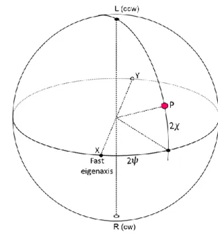
Each oscillation state or orbit of the pendulum bob, as described by figure A1, corresponds to a point P on the surface of the anisosphere of figure A2. The evolution of the orbit orientation and shape as a function of time results in a particular curve, the phase curve, described by the representative point P on the anisosphere.

The equator of the anisosphere is the locus of the points representing planar pendulum orbits projected as rectilinear oscillations on a horizontal plane, in such a way that the longitude along the equator equals twice the swinging azimuth 𝜓 ; (0 ≤ 𝜓 < 180°). Therefore, orthogonal azimuths parallel to the respective axes of a laboratory coordinate system XY will determine on the anisosphere equator the longitudes of two diametrically opposed points, X and Y. The longitude 2𝜓 is counted positive ccw when looking toward the anisosphere centre from above its upper pole L.

The latitude 2𝜒 of point P is twice the inverse tangent of the minor-to-major axis ratio of the ellipse. Positive latitudes (upper hemisphere) represent ellipses described in the ccw direction by the bob. Then pole L represents a ccw circular orbit. Similarly, the lower hemisphere represents all the cw ellipses and the lower pole R represents a cw circular orbit.

(9)

Figure A1. Pendulum orbit as seen from

suspension point. The parameters of orbit orientation are referred to the linear anisotropy axes. X represents the fast eigenaxis, namely the azimuth of shortest swinging period.

Figure A2. The ccw ellipse of figure A1 is

represented by the surface point P whose longitude is twice the azimuth measured from the fast axis X, and whose latitude is twice the inverse tangent of the minor-to-major axis ratio.

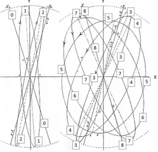
Figure A3 is a composite of figures 5 and 6 in KO’s thesis where, contrary to the adopted conventions for the anisosphere, the fast and slow eigenaxes are labelled y and x respectively. The anisotropy characteristics leading to the 9 orbits of this example have been incorporated into the anisosphere of figure A4. The initial state labelled 0 is rectilinear at an azimuth 17.5 higher than the slow eigenaxis azimuth Y (or x in KO’s original figure). It is seen that the orbit major axis oscillates about the slow axis, so that orbit 8 finally falls back onto orbit 0.

The parameters of KO’s pendulum for pure circular anisotropy are incorporated into figure A4 as axial angular velocity vectors proportional to the rates of increase of the phase difference between the two components of any oscillation resolved along the appropriate eigenstates, namely the ccw (L) and cw (R) circular orbits. Those for pure linear anisotropy are incorporated as vectors lying in the equatorial plane along the diametral axis XY. Pure circular (Foucault) anisotropy is represented by the polar vector whose magnitude is the rate of phase change 2𝜌̇ (twice the Foucault precession rate) and which is pointing toward the faster circular eigenstate R. Pure linear anisotropy is represented by the equatorial vector whose magnitude is 𝛿̇ = 𝜔𝑋− 𝜔𝑌 =

2𝜋(𝑇_𝑌 − 𝑇_𝑋 )/𝑇2_{, and which is pointing toward the faster rectilinear eigenstate X .}

The effect of pure circular anisotropy of the Foucault type in the Northern earth hemisphere is a rotation of the representative point P about the polar axis in a ccw sense when looking toward the centre from above the faster eigenstate R (bird’s eye view), or a rotation of the representative point

P about the polar axis in a cw sense when looking toward the centre from above the slower

eigenstate L.

The effect of pure linear anisotropy is a ccw rotation of the representative point P about the equatorial axis XY when looking toward the centre from above the faster eigenstate X, or a cw rotation of the representative point P about the equatorial axis XY when looking toward the centre from above the slower eigenstate Y.

(10)

(a) (b)

Figure A3. Composite picture from figures 5 and

6 in KO’s thesis, with the anisotropy parameter 𝜓′_{= 30}__{and the initial condition parameter}

𝜀 = 135. The ellipses have been re-annotated for better legibility. KO’s x-axis was the slow eigenaxis (point Y on the anisosphere). Linear anisotropy amounts then to √3 times the amount of Foucault circular anisotropy in that example. Note that ellipses 2 and 5 have practically the same azimuth, and the same holds for ellipses 6 and 7. (a) Normal sub-period with cw ellipses and precession in the Foucault sense. (b) Abnormal sub-period with ccw ellipses and precession mostly in the anti-Foucault sense.

Figure A4. Perspective view of the 9 orbits of

figure A3 on the anisosphere. 𝜀 is the great arc distance from fast eigenstate

M to point 0 representing the initial pendulum

state. The orbit representative point travels cw at constant angular speed on the phase circle. The radius of the phase circle about the slow eigenstate N is a great circle arc equal to 𝜋 − ε = 45 . In this example, the phase period (or KO period) lasts for 8.03 h and comprises one normal sub-period (in red, lower hemisphere), monotonously in the Foucault sense, and one abnormal sub-period (in blue, upper hemisphere), where precession is against the Foucault sense for part of its duration.

When both types of anisotropy are present, the two angular velocity vectors add up to yield a resultant along a new diametral axis joining the elliptical eigenstates N and M, with magnitude Δ̇ = [δ̇2_{+ (2𝜌̇)}2_]1/2_{and pointing toward the faster eigenstate M. The effect of such elliptical}

anisotropy is a ccw rotation of the representative point P about the diametral axis MN when looking toward the centre from above the faster eigenstate M, or a cw rotation of the representative point P about the diametral axis MN when looking toward the centre from above the slower eigenstate N.

The three situations above strictly apply to the 2D linear oscillator. P describes then a small circle centred on the diametral axis, the phase circle, since the increasing rotation angle is the increasing phase difference between the fast and the slow eigenstates as time runs. It will be shown in further publications that for 2D nonlinear oscillators, the phase curve is no longer a small circle and, in some cases, not a closed curve.

7. References

(11)

[2] Kamerlingh Onnes H 1879 Nieuwe bewijzen voor de aswenteling der aarde (Groningen, NL:

J B Wolters, also: U. Groningen)

[3] Verreault R 2018 The anisosphere model: a novel differential phase space representation for Foucault pendulums and 2D oscillators Preprint at this ICM2 Conf.

[4] Verreault R 2017 Eur. Phys. J. Appl. Phys. 79 31001 epjap/2017160337

[5] Allais M 1997 L’Anisotropie de l’Espace (Paris: Clément Juglar), p 95 : graph IV [6] Saxl E J and Allen M 1971 Phys. Rev. D 3 823-825