Bootstrapping the GMM overidentification test Under first-order underidentification

Texte intégral

(1)2014s-25. Bootstrapping the GMM overidentification test Under first-order underidentification Prosper Dovonon, Sílvia Gonçalves. Série Scientifique Scientific Series. Montréal Avril 2014. © 2014 Prosper Dovonon, Sílvia Gonçalves. Tous droits réservés. All rights reserved. Reproduction partielle permise avec citation du document source, incluant la notice ©. Short sections may be quoted without explicit permission, if full credit, including © notice, is given to the source..

(2) CIRANO Le CIRANO est un organisme sans but lucratif constitué en vertu de la Loi des compagnies du Québec. Le financement de son infrastructure et de ses activités de recherche provient des cotisations de ses organisations-membres, d’une subvention d’infrastructure du Ministère de l'Enseignement supérieur, de la Recherche, de la Science et de la Technologie, de même que des subventions et mandats obtenus par ses équipes de recherche. CIRANO is a private non-profit organization incorporated under the Québec Companies Act. Its infrastructure and research activities are funded through fees paid by member organizations, an infrastructure grant from the Ministère de l'Enseignement supérieur, de la Recherche, de la Science et de la Technologie, and grants and research mandates obtained by its research teams. Les partenaires du CIRANO Partenaire majeur Ministère de l'Enseignement supérieur, de la Recherche, de la Science et de la Technologie Partenaires corporatifs Autorité des marchés financiers Banque de développement du Canada Banque du Canada Banque Laurentienne du Canada Banque Nationale du Canada Banque Scotia Bell Canada BMO Groupe financier Caisse de dépôt et placement du Québec Fédération des caisses Desjardins du Québec Financière Sun Life, Québec Gaz Métro Hydro-Québec Industrie Canada Intact Investissements PSP Ministère des Finances et de l’Économie Power Corporation du Canada Rio Tinto Alcan Transat A.T. Ville de Montréal Partenaires universitaires École Polytechnique de Montréal École de technologie supérieure (ÉTS) HEC Montréal Institut national de la recherche scientifique (INRS) McGill University Université Concordia Université de Montréal Université de Sherbrooke Université du Québec Université du Québec à Montréal Université Laval Le CIRANO collabore avec de nombreux centres et chaires de recherche universitaires dont on peut consulter la liste sur son site web. Les cahiers de la série scientifique (CS) visent à rendre accessibles des résultats de recherche effectuée au CIRANO afin de susciter échanges et commentaires. Ces cahiers sont écrits dans le style des publications scientifiques. Les idées et les opinions émises sont sous l’unique responsabilité des auteurs et ne représentent pas nécessairement les positions du CIRANO ou de ses partenaires. This paper presents research carried out at CIRANO and aims at encouraging discussion and comment. The observations and viewpoints expressed are the sole responsibility of the authors. They do not necessarily represent positions of CIRANO or its partners.. ISSN 2292-0838 (en ligne). Partenaire financier.

(3) Bootstrapping the GMM overidentification test Under first-order underidentification Prosper Dovonon *, Sílvia Gonçalves †. Résumé/abstract The main contribution of this paper is to study the applicability of the bootstrap to estimating the distribution of the standard test of overidentifying restrictions of Hansen (1982) when the model is globally identified but the rank condition fails to hold (lack of first order local identification). An important example for which these conditions are verified is the popular test of common conditionally heteroskedastic features proposed by Engle and Kozicki (1993). As Dovonon and Renault (2013) show, the Jacobian matrix for this model is identically zero at the true parameter value, resulting in a highly nonstandard limiting distribution that complicates the computation of critical values. We first show that the standard bootstrap method of Hall and Horowitz (1996) fails to consistently estimate the distribution of the overidentification restrictions test under lack of first order identification. We then propose a new bootstrap method that is asymptotically valid in this context. The modification consists of adding an additional term that recenters the bootstrap moment conditions in a way as to ensure that the bootstrap Jacobian matrix is zero when evaluated at the GMM estimate. Mots clés/Key words: Bootstrapping, overidentification, overidentification. * †. Concordia University, [email protected]. Université de Montréal..

(4) 1. Introduction. GMM estimators are commonly used in economics to estimate parameters defined by moment conditions. Under standard regularity conditions, including the rank identification condition, the GMM √ estimator is T -consistent and asymptotically normal, as shown by Hansen (1982) in his seminal paper. Nevertheless, the bootstrap is often used to estimate the distribution of the GMM estimator and related test statistics because the first order asymptotic distribution is a poor approximation to the GMM finite sample distribution for the sample sizes typically found in practice. The main goal of this paper is to study the applicability of the bootstrap for GMM inference when the standard rank identification condition fails but the model is still globally identified. Global identification, which requires that a unique parameter value θ0 solves the moment conditions, ensures that the GMM estimator is consistent for θ0 . As is well known, global identification is equivalent to the rank identification condition for linear models. The rank identification condition, which requires that the expected value of the Jacobian matrix of the moment conditions with respect to θ is of full column rank, is an example of a local identification condition that is important to derive the first order asymptotic distribution of the GMM estimator. For nonlinear models, and as first discussed by Sargan (1983), it is possible to mantain global identification of the model and at the same time have a rank deficient Jacobian matrix. Failure of the rank identification condition (or first order underidentification) implies that the first order asymptotic distribution of the GMM estimator and related test statistics are highly nonstandard, thus motivating the use of the bootstrap as an alternative method of inference. In this paper, we focus on bootstrapping the test of overidentification restrictions proposed by Hansen (1982) when the model is globally identified but the expected Jacobian matrix is identically zero. Our motivation for considering this special case of rank deficiency is the test for common conditionally heteroskedastic factors studied by Dovonon and Renault (2013) (henceforth D&R (2013)), for which the expected Jacobian matrix is nil when evaluated at the true parameter value. In this case, local identification is ensured by imposing identification conditions on higher order derivatives of the moment conditions. Under these conditions, D&R (2013) show that this popular test (which amounts to a test of appropriately defined overidentifying restrictions) is no longer asymptotically distributed as a χ2H−p random variable (where H denotes the number of moment conditions and p the number of parameter coefficients in θ). Instead, its asymptotic distribution is a fifty-fifty mixture of χ2H−1 and χ2H when p = 1, leading to an oversized test under the null of no common conditionally heteroskedastic features when the standard χ2H−1 distribution is used, independently of the sample size. When p > 1, the correct asymptotic distribution is the minimum of a certain stochastic process whose distribution is highly nonstandard, implying that critical values are difficult to obtain. Our main goal here is to propose a bootstrap method that is able to estimate the correct distribution of the overidentification test in this context. The bootstrap will be especially useful when p > 1 because it avoids the use. 2.

(5) of conservative critical values, which were proposed by D&R (2013) based on their proof that the asymptotic distribution of the test lies between χ2H−p and χ2H when p > 1. Our contributions are as follows. First, we show that the standard bootstrap overidentification test statistics (as proposed by Hall and Horowitz (1996)), where one resamples the moment conditions recentered around the bootstrap population mean evaluated at the GMM estimate θˆT , is not valid when the Jacobian matrix is degenerate. The reason for this failure is that the bootstrap Jacobian matrix is the sample Jacobian matrix evaluated at θˆT and this is typically not zero. Thus the standard GMM bootstrap does not mimic the degeneracy of the expected Jacobian matrix at θ0 . To remedy this problem, we propose two alternative bootstrap methods where the bootstrap GMM estimator is defined as the minimum of a quadratic form of a set of modified recentered bootstrap moment conditions. The first modification that we propose consists on recentering the moment condition that the bootstrap resamples twice: first we subtract off the bootstrap mean of the bootstrap moment conditions evaluated at θˆT , as proposed by Hall and Horowitz (1996). Second, we subtract off a term that is equal to the sample Jacobian matrix evaluated at θˆT multiplied by the difference between θ and θˆT . We label this the corrected bootstrap. The second modification differs from the first one by letting the Jacobian matrix be evaluated at the unknown parameter. Because of its continuous correction nature, we label this as the continuously corrected bootstrap. In both alternatives, the modified bootstrap moment conditions are equal to zero when evaluated at θˆT (as in Hall and Horowitz (1996)), but in addition are such that the first order derivative with respect to θ is zero when evaluated at θˆT . Consequently, the bootstrap expected Jacobian matrix is degenerate and this restores the asymptotic validity of the bootstrap for estimating the overidentification test when the expected Jacobian matrix is zero under the true model. The rest of this paper is organized as follows. In Section 2, we introduce our assumptions and provide the asymptotic distribution of the overidentification test when the expected Jacobian matrix is zero. These results generalize some of the results in D&R (2013) by allowing for general nonlinear moment conditions that are not necessarily quadratic in θ. Section 3 establishes the invalidity of the standard bootstrap method for the test of overidentification conditions when first order underidentification holds. Section 4 introduces the new bootstrap methods based on the doubly recentered bootstrap moment conditions and proves their asymptotic validity. Section 5 contains Monte Carlo simulation results and Section 6 concludes. Two mathematical appendices contain the proofs.. 2. Setup, assumptions and asymptotic theory. We consider a sample {Xt : t = 1, . . . , T } of random variables described by the moment conditions E(ψ(Xt , θ)) = 0,. 3. (1).

(6) where ψ(·, ·) ∈ RH is a known function and θ ∈ Θ ⊂ Rp is the parameter of interest. In the following, we will often write ψt (θ) ≡ ψ (Xt , θ) whenever convenient. Letting QT (θ) ≡ ψ¯T′ (θ)WT ψ¯T (θ), where ψ¯T (θ) =. 1 T. ∑T. t=1 ψ(Xt , θ). and WT a symmetric positive definite random matrix, we can define. the GMM estimator θˆT as θˆT = arg min QT (θ) . θ∈Θ. The statistic of interest is JˆT = T ψ¯T′ (θˆT )WT ψ¯T (θˆT ). When WT is such that WT →P W = Σ−1 , where Σ = Var (ψ(X1 , θ0 )), we obtain the standard Hansen’s (1982) GMM overidentification test statistic. Our aim in this section is to derive the asymptotic distribution of JˆT whenever the Jacobian matrix of the moment conditions is identically zero. An important example that fits into this framework is the test for common conditionally heteroskedastic features recently analyzed by D&R (2013). Our results in this section extend the results of D&R (2013) by considering more general moment conditions (which in particular are not necessarily quadratic in θ).. 2.1. Assumptions. Our assumptions are as follows. Assumption 1 (DGP) Let (Ω, F, P ) denote a complete probability space. We observe an i.i.d. { } sample given by Xt : Ω → Rl , l ∈ N, t = 1, . . . , T . Assumption 2 (global identification) θ0 is an interior point of Θ, a compact subset of Rp , p ∈ N, and it is the unique solution in Θ to the equation E (ψ (Xt , θ)) = 0. Assumption 3 (regularity conditions on ψ) (i) {ψ (x, θ)} is continuous on Θ for all x in the support of X1 . (ii) E (supθ∈Θ ∥ψ (X1 , θ)∥) < ∞. ( ) (iii) E ∥ψ(X1 , θ0 )∥2 < ∞ and Σ ≡ Var (ψ(X1 , θ0 )) is positive definite. Assumption 4 (regularity conditions on derivatives on ψ) (i) {ψ (x, θ)} is twice continuously differentiable with respect to θ in a neighborhood N of θ0 for all x in the support of X1 and there exists a function m (x) such that E(m(X1 )) < ∞ and for ∂ 2 ψh. ∂ 2 ψh any θ1 , θ2 ∈ N , ∂θ∂θ ′ (x, θ1 ) − ∂θ∂θ ′ (x, θ2 ) ≤ m(x)∥θ1 − θ2 ∥, for h = 1, . . . , H, for all x in the support of X1 . 4.

(7) ) ( ( 2 2 ) ∂. (ii) E ∂θ∂ ′ ψ(X1 , θ0 ) < ∞ and E ∂θ∂θ < ∞, for h = 1, . . . , H. ′ ψh (X1 , θ0 ) P. Assumption 5 (weighting matrix) WT → W , a symmetric positive definite matrix. Assumption 6 (local identification) (. ). = 0, where ρ (θ) ≡ E (ψ (X1 , θ)) . [ ( 2 ) ] ∂ (ii) ∀θ ∈ Θ, (θ − θ0 )′ E ∂θ∂θ ψ (X , θ ) (θ − θ ) = 0 ⇐⇒ θ = θ0 . ′ h 1 0 0 (i) E. ∂ ∂θ′ ψ(X1 , θ0 ). =. ∂ ∂θ′ ρ (θ0 ). 1≤h≤H. Assumptions 1, 2, 3 and 5 are standard in the GMM literature but Assumptions 4 and 6 are not. Assumption 4(i) is useful to control the remainder of second-order Taylor expansions of the estimating function while the first part of Assumption 4(ii) ensures the applicability of some central limit theorem to the sample mean of the Jacobian matrix of the estimating function evaluated at the true value θ0 . The second part of Assumption 4(ii) along with Assumption 4(i) ensures that the second order derivatives of the estimating function is uniformly dominated in a neighborhood of θ0 allowing for the application of the uniform law of large numbers. Part (i) of Assumption 6 states that the expected value of the Jacobian matrix is zero. This is a violation of the standard rank identification condition, which requires the rank of. ∂ ∂θ ′ ρ (θ0 ). to be equal to p. Given the lack of first order identification, part. (ii) of Assumption 6 ensures local identification of θ0 through second-order derivatives. In particular, letting G≡. [. ( vec. ∂ 2 ρ1 (θ0 ) ∂θ∂θ ′. ). ···. ( vec. ∂ 2 ρH (θ0 ) ∂θ∂θ′. ) ]′. denote an H × p2 matrix, Assumption 6(ii) is equivalent to ( ) Gvec (θ − θ0 )(θ − θ0 )′ ̸= 0 for all θ ̸= θ0 . When p = 1, (2) is equivalent to G ̸= 0, i.e.. ∂ 2 ρh (θ0 ) ∂θ2. (2). ̸= 0 for at least one h = 1, . . . , H. In the general. case, the condition that G ̸= 0 is obviously necessary for (2) but it is not sufficient. It is hard to provide more primitive conditions in this case as this amounts to giving conditions for a unique solution of a set of H nonlinear equations in θ. An important example that satisfies (2) are the moment conditions underlying the test for common conditionally heteroskedastic features. See D&R’s (2013) Lemma 2.3. Next, we derive the asymptotic distribution of JˆT under Assumptions 1-6.. 2.2. Asymptotic results. Proposition 2.1 Under Assumptions 1-3 and 5, θˆT − θ0 = oP (1) . Proposition 2.1 shows that the GMM estimator is consistent for θ0 despite the lack of first order identification. This is an immediate consequence of global identification and the uniform convergence of QT (θ) towards Q (θ) = E (ψ (Xt , θ))′ W E (ψ (Xt , θ)) ≡ ρ (θ)′ W ρ (θ) , 5.

(8) where ρ (θ) ≡ E (ψ (Xt , θ)) . Our next result derives the rate of convergence of θˆT − θ0 when local identification is achieved through second-order local conditions.. ( ) ( ). Proposition 2.2 Under Assumptions 1-6, (i) θˆT − θ0 = OP T −1/4 and (ii) T 1/4 θˆT − θ0 has at least a subsequence that converges in distribution to some random variable V such that P (V ̸= 0) > 0. Part (i) of Proposition 2.2 shows that the convergence rate of θˆT − θ0 is at least T −1/4 whereas ( ) part (ii) shows that this rate is sharp, i.e. there is a subsequence of T 1/4 θˆT − θ0 which converges ) ( in distribution to a nondegenerate random variable V . This implies that T 1/4 θˆT − θ0 cannot be oP (1) (if it were then any subsequence would converge in distribution to 0).. √ T rate of conver( ) √ gence, note that we can write a second-order Taylor expansion of the moment conditions T ψ¯T θˆT To understand why the lack of first order identification implies a slower than. as. ) ( ) ( ) √ √ 1 ∂ ψ¯T (θ0 ) √ ( ˆ θ − θ + R θ¨T , T ψ¯T θˆT = T ψ¯T (θ0 ) + T 0 T T ′ ∂θ 2 | {z }. (3). =oP (1) under Assumption 6(i). where the remainder is such that ( ) ( ) ¯ θ¨T RT θ¨T = G | {z } ↓P G. ( ( ) ( )′ ) 1/4 ˆ 1/4 ˆ vec T θT − θ0 T θT − θ0 ,. under A6(ii). where for any θ, ¯ (θ) ≡ G. [. ( vec. ∂ 2 ψ¯1,T (θ) ∂θ∂θ′. ). ···. ( vec. ∂ 2 ψ¯H,T (θ) ∂θ∂θ′. ) ]′. (4). √ ¯T (θ0 ) = OP (1) (by a CLT) and is a random H × p2 matrix. Because the Jacobian matrix is nil, T ∂ ψ∂θ ′ since θˆT − θ0 = oP (1), it follows that the second term in (3) is oP (1). Thus, identification is achieved ( ) at the second-order. In particular, Assumption 6(ii) guarantees that RT θ¨T is an OP (1) term that ( ) is not oP (1), implying that T 1/4 θˆT − θ0 = OP (1) . To describe the asymptotic distribution of JˆT we need to introduce some additional notation. Following D&R (2013), let ( ZT (θ0 ) =. ) ∂ 2 ρ′ (θ0 ) √ ¯ W T ψT (θ0 ) ∂θi ∂θj 1≤i,j≤p. denote a symmetric random p × p matrix whose limit in distribution is given by the following random Gaussian matrix. ( Z(X) =. ∂ 2 ρ′ (θ0 ) WX ∂θi ∂θj. 6. ) , 1≤i,j≤p.

(9) with X ∼ N (0, Σ). Similarly, define the Rp -indexed stochastic process ( ) 1 ( ) ( ) J (v) ≡ X ′ W X + X ′ W Gvec vv ′ + vec′ vv ′ G′ W Gvec vv ′ , 4 where v ∈ Rp and note that the sample paths of J are continuous functions of v. Theorem 2.1 If Assumptions 1-6 hold, then as T → ∞, d JˆT → J ≡ minp J(v). v∈R. and x → P (J ≤ x) is continuous at x, for all x ∈ R. The first part of Theorem 2.1 extends Theorem 3.1 of D&R (2013) to the case of general moment conditions satisfying Assumptions 1-6. In particular, we do not restrict ourselves to quadratic functions of θ. The second part of this theorem is new. It shows that the asymptotic distribution of JT is continuous. This result is essential to prove that the bootstrap methods that we introduce in this paper (see Sections 4) are uniformly consistent. Regarding the first part of Theorem 2.1, the main insights of D&R’s (2013) proof remain valid here. Specifically, we consider the following stochastic process indexed by v ∈ Rp ,. ( ) ( )′ JT (v) = T ψ¯T θ0 + T −1/4 v WT ψ¯T θ0 + T −1/4 v ,. where v is implicitly defined as v = T 1/4 (θ − θ0 ), with θ ∈ Θ. Let ℓ∞ (K) denote the space of bounded real-valued functions on a compact subset K ⊂ Rp , equipped with the supremum norm supv∈K |z (v)|.1. We show in the Appendix that JT ⇒ J in ℓ∞ (K) for every compact K ⊂ Rp ,. which is equivalent to Eh (JT ) → E (h (J)), for any h : ℓ∞ (K) → R bounded and continuous ( ) with respect to the sup norm. Let vˆT = T 1/4 θˆT − θ0 . Since JˆT = JT (ˆ vT ) = minv∈HT JT (v), { } where HT ≡ v ∈ Rp : v = T 1/4 (θ − θ0 ) , θ ∈ Θ is such that ∪T ≥0 HT = Rp , uniform tightness of vˆT ∈ arg minv∈HT JT (v) and of vˆ ∈ arg minv∈Rp J(v) suffice to show that the minimum of JT (v) converges in distribution to the minimum of J (v) (see Lemma B.5 of D&R (2013)). Theorem 2.1 provides the asymptotic distribution for the GMM overidentification test statistic JˆT under second-order identification (the standard case where WT →P W = Σ−1 is included as a special case). As it makes clear, and as was already discussed by D&R (2013) in the context of the test for common conditionally heteroskedastic features, the lack of first order identification implies that this distribution is no longer the standard chi-squared distribution with H − p degrees of freedom. Instead, the correct distribution of JˆT is the distribution of J which, as we show in this paper, is continuous. Except for the special case when p = 1, for which D&R (2013) showed that this distribution is a fifty-fifty mixture of χ2H and χ2H−1 , critical values of J are not available. This is the main motivation for proposing the bootstrap. 1. Note that for given ω ∈ Ω, the sample paths of v 7→ J (ω, v) and v 7→ JT (ω, v) , v ∈ K are elements of ℓ∞ (K).. 7.

(10) 3. Asymptotic invalidity of the standard bootstrap. Given Assumption 1, we let {Xt∗ : t = 1, . . . , T } denote a (conditionally) i.i.d. bootstrap sample obtained by resampling with replacement the original sample XT .2 A standard application of the bootstrap for GMM estimators involves recentering the bootstrap moment conditions by subtracting the ( ( )) ∑ term3 E ∗ ψ Xt∗ , θˆT from T1 Tt=1 ψt (Xt∗ , θ) when defining the bootstrap criterion function, i.e. ∗ ∗ Q∗T (θ) = ψ¯c,T (θ)′ WT∗ ψ¯c,T (θ) ,. where WT∗ is a symmetric positive definite weighting matrix that may depend on the bootstrap sample and ∗ ψ¯c,T (θ) = T −1. T ∑. ψc (Xt∗ , θ) , with. t=1. ψc (Xt∗ , θ). ( ( )) = ψ (Xt∗ , θ) − E ∗ ψ Xt∗ , θˆT .. ∗ (θ) ≡ ψ (X ∗ , θ) for t = 1, . . . , T and θ ∈ Θ, it follows that Letting ψt∗ (θ) ≡ ψ (Xt∗ , θ) and ψc,t c t ( ( )) ψ ∗ (θ) = ψ ∗ (θ) − E ∗ ψ ∗ θˆT . c,t. t. t. Recentering ensures that the bootstrap moment conditions are equal to zero when evaluated at the ( ( )) ∗ “true parameter” θˆT , i.e. that we have E ∗ ψ¯c,T θˆT = 0. Instead, by the properties of the i.i.d. bootstrap, without recentering, we have that ) ( T T T ( ) ) ∑ 1 ∑ (ˆ ) 1∑ ( 1 ∗ ˆ ∗ = ψt θ T ψt θT = ψ Xt , θˆT , E T T T t=1. t=1. t=1. which is not necessarily zero when the model is overidentified. As shown by Hahn (1996), recentering of the moment conditions in the bootstrap world is not necessary for the consistency of the bootstrap distribution of the bootstrap GMM estimator. Nevertheless, it is important to obtain asymptotic refinements for bootstrap tests and intervals based on Wald tests, as first shown by Hall and Horowitz (1996) and further studied by Andrews (2002) and Inoue and Shintani (2006), among others. For bootstrapping the distribution of the overidentification test, recentering is crucial even for first-order asymptotic validity of the bootstrap. This was discussed by Brown and Newey (2002), who proposed using a weighted bootstrap scheme, where the bootstrap probabilities are the implied empirical likelihood probabilities instead of the empirical probabilities given by 1/T. The goal of this section is to study the asymptotic properties of the standard GMM bootstrap Under weak dependence of {Xt : t = 1, . . . , T }, a block bootstrap would be appropriate. We do not consider this possibility here because our focus is on the impact of the first order local underidentification on bootstrap validity rather than on the impact of weak dependence. 3 Here and throughout, we let E ∗ , V ar∗ and P ∗ denote the bootstrap expectation, variance and probability measure induced by the resampling, conditional on the original sample. Appendix B gives more details on these bootstrap definitions. 2. 8.

(11) when local identification is achieved at the second-order as described by Assumption 5. The bootstrap GMM estimator and the corresponding overidentification test statistic are defined as ( ) ( ) ∗′ ∗ θˆT∗ = arg min Q∗T (θ) and JˆT∗ = T ψ¯c,T θˆT∗ WT∗ ψ¯c,T θˆT∗ . θ∈Θ. We require WT∗ to converge to W under the bootstrap measure P ∗ with probability P approaching ∗. one, i.e. WT∗ →P W in prob-P (see Appendix B for the formal definition of this mode of convergence). Remark 1 below provides more discussion on how to choose WT∗ in practice. Our first result shows that θˆT∗ is consistent for θ0 under P ∗ with probability approaching one. Given Proposition 2.1, this result implies the usual result that θˆ∗ is consistent for θˆT in probability. T. ∗ Proposition 3.1 Under Assumptions 1-6 and if WT∗ →P W in prob-P , then θˆT∗ − θ0 = oP ∗ (1) in. prob-P . The proof of this result is rather standard and requires showing that supθ∈Θ |QT (θ) − Q (θ)| = oP (1) and supθ∈Θ |Q∗T (θ) − QT (θ)| = oP ∗ (1) in prob-P . This together with the fact that θ0 is the unique solution to the moment conditions ρ (θ) = 0 (and hence the unique minimizer of Q (θ) over Θ) deliver the result. Our next result shows that the standard GMM bootstrap method does not consistently estimate the distribution of JˆT . Specifically, we show that the unconditional limiting distribution of the bootstrap overidentification statistic JˆT∗ does not coincide with the asymptotic distribution of JˆT . To simplify the arguments, we consider only the case where p = 1, but the asymptotic invalidity of the standard bootstrap method extends to the general case p > 1. Because our proof of invalidity is based on the unconditional distribution of JˆT∗ , we need to introduce the joint probability measure P = P × P ∗ that accounts for the two sources of randomness in Jˆ∗ : T. the randomness that comes from the original data (and which is described by P ) and the randomness that comes from the resampling, conditional on the original sample (described by P ∗ ). See Appendix B for more details on the properties of P and its relation to P ∗ and P . To characterize the bootstrap distribution of JˆT∗ , we introduce the following stochastic process indexed by v ∈ R,. ( )′ ( ) ∗ ∗ JT∗ (v) = T ψ¯c,T θˆT + T −1/4 v WT∗ ψ¯c,T θˆT + T −1/4 v , ( ) where v is implicitly defined as v = T 1/4 θ − θˆT , with θ ∈ Θ. Note that JˆT∗ = JT∗ (ˆ vT∗ ) = min JT∗ (v) , {. (. where VT = v ∈ R : v = T 1/4 θ − θˆT. ). v∈VT. } ,θ ∈ Θ .. Theorem 3.1 Suppose that the assumptions of Proposition 3.1 hold with p = 1. It follows that:. ( ). (i) θˆT∗ − θ0 = OP T −1/4 . 9.

(12) (ii) There exists at least one subsequence of (√ ( ) ( )) √ ( ) T ψ¯T (θ0 ) , T ψ¯T∗ (θ0 ) − ψ¯T (θ0 ) , T 1/4 θˆT − θ0 , T 1/4 θˆT∗ − θˆT which converges in distribution under P towards (X, X ∗ , V, U ∗ ), where X and X ∗ have the same distribution N (0, Σ), X ∗ is independent of (X, V ), and P (U ∗ ̸= 0) > 0. (iii) Along that same subsequence, JˆT∗ converges in distribution under P towards J ∗ ≡ minv∈R J ∗ (v), where. ( )′ ( ) ( )′ 1 1 1 1 ∗ 2 ∗ 2 ∗ 2 J (v) = X − GV W X − GV + X − GV W Gv 2 + G′ W Gv 4 . 2 2 2 4 ∗. (iv) If, in addition, W = Σ−1 , then E(J ∗ ) = E(J) −. 1 2π .. Part (i) of Theorem 3.1 shows that the convergence rate of θˆT∗ − θ0 is T −1/4 whereas part (ii) shows that this rate is sharp. Thus, the standard bootstrap method replicates the convergence rate of the GMM estimator despite first order underidentification. Nevertheless, and as shown by part (iii), the limit process of JT (v) does not look like the unconditional limit of the bootstrap process JT∗ (v) since √ the latter depends on V 2 , the limit distribution of T (θˆT − θ0 )2 . This is a strong indication that the minima (J, and J ∗ ) of these limit processes may not have the same distribution; highlighting the invalidity of this standard bootstrap method. This is precisely the point made by part (iv) which, for W = Σ−1 , shows that the expected values of these minima differ by 1/2π, which in particular implies that the standard bootstrap distribution is asymptotically biased. The main reason for the failure of the standard bootstrap when applied to the overidentification test is that while the sample mean of the Jacobian matrix of the estimating function evaluated at the ¯ 0 )/∂θ′ , is of order OP (T −1/2 ), its bootstrap analogue is of order OP (T −1/4 ). population value θ0 , ∂ ψ(θ This rate is not fast enough to make the terms depending on this Jacobian matrix vanish from the expansion of the bootstrap test statistic, creating a discrepancy between the limiting distributions of the original statistic and its bootstrap analogue.. 4. Modified bootstrap moment conditions. In this section, we propose two alternative modifications to the standard GMM bootstrap. Both alternatives involve a double recentering of the bootstrap moment conditions. This double recentering ensures that not only the bootstrap expected value of the bootstrap moment conditions at θˆT is zero, but that the bootstrap expected Jacobian matrix at θˆT is also zero.. 4.1. The corrected GMM bootstrap. The first method considers the following bootstrap moment conditions, ( ) ( ( )) ) ∂ ∗ (ˆ ) ( ∗(1) ∗ ∗ ∗ ˆ ∗ ˆT , ψt (θ) = ψt (θ) − E ψt θT ψ −E θ θ − θ T t ∂θ′. 10.

(13) ∗(1). where ψt. (θ) ≡ ψ (1) (Xt∗ , θ) for any t = 1, . . . , T and θ ∈ Θ. Thus, we recenter the original boot-. strap moment function ψt∗ (θ) = ψ (Xt∗ , θ) twice: first by subtracting off its bootstrap expected value evaluated at θˆT (as in the standard GMM bootstrap), and second by subtracting off the product of the expected bootstrap Jacobian matrix evaluated at θˆT with the factor θ − θˆT . We call this method the “corrected” GMM bootstrap. Similarly to the standard GMM bootstrap, we have that ( ( )) ∗(1) ˆ E ∗ ψt θT = 0, ( ) ∑ ∗(1) ∗(1) ∗(1) which ensures E ∗ ψ¯T (θ) = 0 when θ = θˆT , where ψ¯T (θ) ≡ T −1 Tt=1 ψt (θ) . Nevertheless, and contrary to the standard GMM bootstrap, the second recentering ensures that the expected value of the bootstrap Jacobian matrix ) ( ) ( ) ( ∂ ∗(1) ∂ ∗ ∂ ∗ (ˆ ) ∗ ∗ ∗ E ψ (θ) = E ψ (θ) − E ψ θT ∂θ′ t ∂θ′ t ∂θ′ t is zero when θ = θˆT . Thus, the corrected GMM bootstrap is able to mimic the lack of first-order identification at θ0 that affects the original moment conditions. Let ∗(1). QT. ∗(1)′ ∗(1) ∗(1) (θ) = ψ¯T (θ) WT ψ¯T (θ) ,. ∗(1). where WT. is a symmetric positive definite weighting matrix that may depend on the bootstrap ∗(1) ∗(1) sample. The modified bootstrap GMM estimator θˆT is defined as the minimum of QT (θ) over θ ∈ Θ. The corresponding overidentification test statistic is given by ( ) ( ) ∗(1) ∗(1)′ ˆ∗(1) ∗(1) ¯∗(1) ˆ∗(1) Jˆ = T ψ¯ θ W ψ θ . T. T. T. T. T. T. ( ) √ ∗(1) ˆ θT /∂θ′ = = 0, the second recentering term ensures that T ∂ ψ¯T √ OP ∗ (1) in prob-P , thus mimicking the fact that T ∂ ψ¯T (θ0 ) /∂θ′ = OP (1) under first order underiWe note that since E ∗. (. ∗(1) ∂ ∂θ ′ ψt. (. θˆT. )). dentification. ∗(1) We first show that θˆT is consistent for θ0 under the bootstrap probability measure P ∗ with. probability approaching one. We impose the additional moment condition, which is a strenghtening of Assumption 4 (ii).. ) (. t ,θ) Assumption 7 E supθ∈Θ ∂ψ(X < ∞. ∂θ′ ∗(1). Proposition 4.1 Under Assumptions 1-7, if WT. ∗ ∗(1) →P W in prob-P , then θˆT = θ0 + oP ∗ (1) in. prob-P . ∗(1) Given Proposition 2.1, Proposition 4.1 implies that θˆT = θˆT + oP ∗ (1) in prob-P. The next result ∗(1) shows that the convergence rate of the bootstrap GMM estimator θˆT is T −1/4 and that this rate is. sharp.. 11.

(14) . ( ) ∗(1). Proposition 4.2 Under the same assumptions as in Proposition 4.1, (i) θˆT − θˆT = OP ∗ T −1/4 ( ) ∗(1) in prob-P , and (ii) T 1/4 θˆT − θˆT has at least a subsequence that converges in distribution to some random variable V ∗ under P ∗ , a.s. -P , such that for some δ > 0, P (∥V ∗ ∥ ̸= 0) ≥ δ. ∗(1). Part (ii) shows that vˆT. ( ) ∗(1) ≡ T 1/4 θˆT − θˆT is not oP ∗ (1) , a.s.-P , which suffices to show that the. ∗(1) rate of convergence derived in (i) is sharp. Next, we show that the modified bootstrap statistic JˆT has the same asymptotic distribution as JˆT , the original test statistic, under first-order underidentification.. To characterize the bootstrap distribution we introduce the following stochastic process indexed by v ∈ Rp ,. )′ ) ( ( ∗(1) ˆ ∗(1) ∗(1) ˆ (v) = T ψ¯T θT + T −1/4 v WT ψ¯T θT + T −1/4 v , ( ) where v is implicitly defined as v = T 1/4 θ − θˆT , with θ ∈ Θ. As before, note that ∗(1). JT. ( ) ∗(1) ∗(1) ∗(1) ∗(1) JˆT = JT vˆT = min JT (v) , v∈VT. where VT. { ( ) } = v ∈ Rp : v = T 1/4 θ − θˆT , θ ∈ Θ . Our first result shows that conditionally on the ∗(1). (v) converges weakly to J (v) in ℓ∞ (K) in probability for every compact ( ( )) ∗ ∗(1) ∗(1) K ⊂ Rp . This is denoted as JT ⇒P J in ℓ∞ (K), in prob-P, and it means that E ∗ h JT → original sample Xn , JT. E (h (J)) in prob-P for any h : ℓ∞ (K) → R bounded and continuous with respect to the sup norm. ∗(1). Lemma 4.1 Under Assumptions 1-7, if WT. ∗. ∗(1). →P W in prob-P , we have that JT. ∗. (v) ⇒P J (v). in ℓ∞ (K) , in prob-P. Lemma 4.1 is instrumental in deriving the following result. ∗(1). ∗. ∗(1) d∗. ˆ Theorem 4.1 Under Assumptions 1-7, if WT →P W in

(15)

(16) prob-P , we have that (i) JT

(17) ∗ ˆ∗(1)

(18) ≤ x) − P (JˆT ≤ x)

(19) → 0, in prob-P. J, in prob-P, and (ii) supx∈R

(20) P (J. → minv∈Rp J(v) ≡. T. Theorem 4.1 shows that the bootstrap distribution of the corrected bootstrap overidentification ∗(1) test statistic Jˆ is consistent for the distribution of the original statistic JˆT . This result justifies using T. the corrected bootstrap method to compute the critical values of JˆT when testing for overidentifying restrictions. This is particularly useful when p > 1, for which there is no closed form expression for the asymptotic distribution of JˆT and the only available alternative is the use of conservative critical values, as proposed by D&R (2013).. 4.2. The continuously-corrected GMM bootstrap. The second modification we consider is based on the following modified moment conditions: )( ( ( ( )) ) ∂ ∗ ∗(2) ∗ ∗ ∗ ˆ ∗ ˆT , ψt (θ) = ψt (θ) − E ψt θT ψ (θ) θ − θ −E ∂θ′ t. 12.

(21) where the expected bootstrap Jacobian matrix is evaluated at θ instead of θˆT . Because this bears a resemblance with the continuous-updated GMM, in which the weighting matrix is evaluated at θ and not at θˆT , we call this method the “continuously-corrected” GMM bootstrap. As our simulations show, the finite sample null rejection rates of this method are closer to desired nominal level than those of the corrected bootstrap method, which is our main motivation for studying its theoretical properties here. ∗(2). The Jacobian matrix of ψh,t (θ) (h = 1, . . . , H) is given by )( ( ( 2 ) ) ∂ ∗(2) ∂ ∗ ∂ ∗ ∂ ∗ ∗ ∗ ˆ ψ (θ) θ − θT − E ψ (θ) = ψ (θ) − E ψ (θ) , ∂θ h,t ∂θ h,t ∂θ∂θ′ h,t ∂θ h,t implying that its bootstrap expectation at θ = θˆT is also equal to zero: ) ( ) ( 2 ( ) ( )) ( ∂ ∗ (ˆ ) ∂ ∂ ∗(2) ( ˆ ) ∗ ∗ ∗ ∗ ˆT − θˆT ˆT θ =E −E ψ θ E ψh,t θT ψh,t θT ∂θ ∂θ ∂θ∂θ′ h,t ( ) ∂ ∗ (ˆ ) −E ∗ = 0. ψ θT ∂θ h,t ∗(2) The set of moment conditions that the “continuously-corrected” GMM bootstrap implements, ψ¯T (θ),. converge uniformly towards a modified set of moment conditions given by ( ) ∂ψ(X1 , θ) E (Φ (X1 , θ)) = E(ψ(X1 , θ)) − E (θ − θ0 ) , ∂θ′ where we let Φ(x, θ) ≡ ψ(x, θ) −. ∂ψ(x, θ) (θ − θ0 ). ∂θ′. To ensure that these modified moment conditions identify θ0 , we need to impose the following assumption. Assumption 8 θ0 is the unique solution to the equation E (Φ (X1 , θ)) = 0. Assumption 8 imposes the restriction that θ0 , the parameter vector that uniquely identifies the original moment conditions given by Assumption 2, also uniquely identifies the modified moment conditions E (Φ (X1 , θ)) = 0. One leading case where this requirement is satisfied is when the original moment conditions ψ (x, θ) are quadratic in θ and and the expected Jacobian matrix is nil at θ0 . Actually, in this case, E(Φ(x, θ)) = −E(ψ(x, θ)), for all θ. Note that the test for common conditionally heteroskedastic features fits into this category. It is also worthwhile to mention that E(Φ(x, θ)) = 0 has the same local identification properties at θ0 as E(ψ(x, θ)) = 0. In particular, we can see that ( ) [ ( 2 ) ] ∂Φ(x, θ0 ) ∂ Φh (x, θ0 ) ′ E = 0, and that (θ − θ ) E (θ − θ ) = 0 ⇔ (θ = θ0 ). 0 0 ∂θ′ ∂θ∂θ′ 1≤h≤H ∗(2) Under Assumptions 1-8, we can show that θˆT , the bootstrap GMM estimator that minimizes ∗(2). QT. ∗(2)′ ∗(2) ∗(2) (θ) = ψ¯T (θ) WT ψ¯T (θ) ,. 13.

(22) ∗(2). over θ ∈ Θ, is consistent towards θ0 . Here and throughout, WT random weighting matrix that converges to W in probability ∗(2). Proposition 4.3 Under Assumptions 1-8, if WT. P ∗,. denotes a symmetric bootstrap. in prob-P .. ∗ ∗(2) →P W in prob-P , then θˆT = θ0 + oP ∗ (1) in. prob-P . ∗(2) Given θˆT , we can form the bootstrap overidentification test statistic ( ) ( ) ∗(2) ∗(2)′ ˆ∗(2) ∗(2) ∗(2) ˆ∗(2) JˆT = T ψ¯T θT WT ψ¯T θT . ∗(2) To show that the bootstrap distribution of JˆT is consistent for the distribution of JˆT , we need to. impose the following additional regularity condition, which strengthens Assumption 4(i). Assumption 9 {ψ (x, θ)} is three times continuously differentiable with respect to θ in a neighbor) (. ∂3 ψ (X , θ) < ∞ for all hood N of θ0 for all x in the support of X1 and E supθ∈N ∂θi ∂θ. 1 j ∂θ i, j = 1, . . . , p. ∗(1) Theorem 4.2 Under Assumptions 1-9, the conclusions of Theorem 4.1 hold with JˆT replaced with ∗ ∗(2) ∗(2) Jˆ provided W →P W in prob-P . T. T. Theorem 4.2 is the analogue of Theorem 4.1 for the continuously-corrected GMM bootstrap. As the proof in Appendix B shows, it follows by establishing the analogues of Proposition 4.2 and Lemma 4.1 for this bootstrap method. Remark 1 (the choice of WT and WT∗ ) In practice, implementing the overidentification test requires the choice of the weighting matrices in the original sample and in the bootstrap samples. The usual practice is to choose WT such that WT →P W = Σ−1 , which amounts to the efficient GMM when the rank condition for identification is satisfied. Under our assumptions, a consistent estimator of Σ−1 is given by the inverse of T 1∑ ψt (θ˜T )ψt (θ˜T )′ , T t=1. where θ˜T is a first-step GMM estimator that is consistent for θ0 (e.g. a GMM estimator based on WT = Ip ). Similarly, one possible choice for WT∗ is the inverse of T 1 ∑ ∗ ˜∗ ∗ ˜ ′ ψt (θT )ψt (θT ) , T t=1. where θ˜T∗ is a first-step GMM estimator based on Ip . Our theoretical results require only that WT∗ is consistent for W, which follows for this particular choice of WT∗ when W = Σ−1 under standard assumptions (since our focus is on the consequences of the rank identification failure for the bootstrap rather than on the implementation of the two-step GMM estimator, we do not provide the particular set of assumptions that justify this choice here). 14.

(23) 5. Monte Carlo simulations. In this section, we illustrate the finite sample properties of the proposed tests in the context of testing for common conditionally heteroskedastic factors. Specifically, we consider an n × 1 return vector Yt+1 with the following conditionally heteroskedastic factor representation, Yt+1 = ΛFt+1 + Ut+1 , where Λ is the matrix of factor loadings, Ft+1 is the vector of conditionally heteroskedastic and mutually independent factors, and Ut+1 is the vector of idiosyncratic shocks. In particular, we let Ut+1 ∼ i.i.d. N (0, 12 I), where I denotes the identity matrix. The generic component ft+1 of Ft+1 follows a Gaussian-GARCH model, ft+1 = σt εt+1 ,. 2 σt2 = ω + αft2 + βσt−1 ; ω, α, β > 0 and εt ∼ i.i.d. N (0, 1).. The null of interest is the null of common conditionally heteroskedastic features. As Engle and Kozicki ( ) (1993) explained, if there exists a parameter vector δ ̸= 0 such that V ar δ ′ Yt+1 |F t is constant (where F t denotes the information set available at time t), then the n return series in Yt+1 share common conditionally heteroskedastic features described by the vector δ. This restriction is a testable restriction. In particular, if zt ∈ F t , we can test for a constant conditional variance of δ ′ Yt+1 by considering the following moment conditions: )) ( (( )2 H0 : E (zt − E(zt )) δ ′ Yt+1 − c (δ) = 0, ( ) where c (δ) ≡ E (δ ′ Yt+1 )2 denotes the unconditional variance of δ ′ Yt+1 . By casting the problem of testing for common features as a GMM testing problem, a natural way to test H0 is to rely on Hansen’s (1982) overidentification test statistic. Nevertheless, and as recently pointed out by D&R (2013), this is precisely an example where the expected Jacobian matrix is zero under H0 . Our goal in this section is to compare the performance of the bootstrap methods studied in this paper with the asymptotic tests studied in D&R (2013). As explained by D&R (2013), in practice, we consider the feasible moment conditions, H0 : E (ψt,T (δ)) = 0 where. ) )2 δ ′ Yt+1 − c¯T (δ) , ∑ where we replace c (δ) with its sample version c¯ (δ) ≡ T −1 Tt=1 (δ ′ Yt+1 )2 . In order to globally identify ∑ δ, a normalization on δ is imposed. We follow D&R (2013) and assume that ni=1 δi = 1 and set ∑ δn = 1 − n−1 i=1 δi in our derivations. ψt,T (δ) ≡ (zt − z¯T ). ((. Our simulation design is as in D&R (2013). In particular, we consider models with n = 2 and 3 asset return series. Designs 1 and 2 generate bivariate return series with 1 and 2 heteroskedastic. 15.

(24) factors, respectively, while Designs 3, 4 and 5 generate trivariate returns with 2, 1 and 3 factors, respectively. Designs 1, 3 and 4 generate returns under the null hypothesis. In particular, Designs 1 and 3 imply the existence of n − 1 common factors whereas Design 4 implies the existence of n − 2 common factors. While our theory does not provide an exact asymptotic distribution for the case of n asset returns with less than n − 1 factors (unless the co-feature vectors are identified through some additional restrictions), this setup is nevertheless of obvious interest in practice. This is why we include Design 4 in our simulations. Designs 2 and 5 imply the existence of no common conditionally heteroskedastic factors and hence allow us to investigate power. The simulation designs are summarized in the following table.. Design 1 Design 2. Number of assets 2 2. Number of factors 1 2. Design 3. 3. 2. Design 4 Design 5. 3 3. 1 3. GARCH Parameters F1 : (ω, α, β) = (0.2, 0.2, 0.6) F1 : (ω, α, β) = (0.2, 0.2, 0.6) F2 : (ω, α, β) = (0.2, 0.4, 0.4) F1 : (ω, α, β) = (0.2, 0.2, 0.6) F2 : (ω, α, β) = (0.2, 0.4, 0.4) F1 : (ω, α, β) = (0.2, 0.2, 0.6) F1 : (ω, α, β) = (0.2, 0.2, 0.6) F2 : (ω, α, β) = (0.2, 0.4, 0.4) F3 : (ω, α, β) = (0.1, 0.1, 0.8). Factor loading (1, 0.5)′ I2 (λ1 |λ2 ): λ1 = (1, 1, 0.5)′ λ2 = (0, 1, 0.5)′ ′ (1, 1, 0.5) I3. ( 2 ) 2 ′ for the designs with 2 The GMM estimations are carried out with H = 2 and zt = Y1,t , Y2,t ( 2 ) 2 , Y 2 ′ for the designs with 3 assets. assets, and with H = 3 and zt = Y1,t , Y2,t 3,t The sample sizes are T = 1000, 2000, 5000, 10, 000, 20, 000, 40, 000 and 50, 000 throughout. Because the convergence rate of the GMM estimator is T 1/4 , it is important to allow for larger than usual sample sizes to evaluate the performance of the methods in this context. The simulation rejection rates are based on 10,000 Monte Carlo replications with 199 bootstrap replications for each Monte Carlo replication throughout. The bootstrap samples consist of random draws with replacement of T realizations from {(Y2 , z1 ), (Y3 , z2 ), · · · , (YT , zT −1 )}. We consider the standard bootstrap and the modified bootstrap methods proposed in Section 4. The choice of the weighting matrices is done as explained in Remark 1 and the nominal level is 5% throughout. Design 1 corresponds to the case where the number p of parameters in δ is equal to 1. Thus, the resulting overidentification test statistic is asymptotically distributed as a fifty-fifty mixture of chi-square distributions with 1 and 2 degrees of freedom. For Design 3, p = 2 and therefore we do not know the critical values of the limiting distribution of JˆT in this case. However, as suggested by D&R (2013), this test can be carried out conservatively using the quantiles from a chi-square distribution with 3 degrees of freedom. The bootstrap methodologies developed in this paper are expected to provide asymptotically correct critical values to perform this test. Design 4 corresponds to a case of common conditionally heteroskedastic factor structure but, without some identifying restrictions on δ, no exact asymptotic distribution is available in the literature for the test statistic and our theory 16.

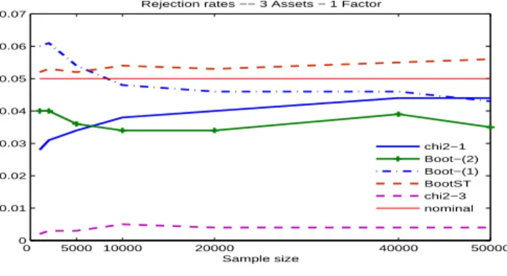
(25) does not apply either. Following D&R (2013), we carry out the simulations without such restrictions to assess the performances of the tests in this case. Designs 2 and 5 correspond to the alternative where no co-feature vector exists and the purpose of these designs is to assess the power of the tests. The results are displayed in Figures 1 through 5. Figure 1 gives the simulated null rejection rates for the bootstrap and asymptotic tests for Design 1 for which critical values for the asymptotic test are available. Results for the standard bootstrap are labeled “BootST”, whereas “Boot-(1)” refers to the corrected bootstrap and “Boot-(2)” refers to the continuously-corrected bootstrap. “Asym” indicates results based on the asymptotic distribution based on the fifty-fifty mixture of χ21 and χ22 . The results confirm the failure of the standard bootstrap reflected by a systematic over-rejection of the null hypothesis of factor structure with a rejection rate at around 8% in large samples. The corrected bootstrap also over-rejects for small sample sizes, but its rejection rate declines as the sample size grows, reaching around 6% for large samples. The continuously-corrected bootstrap tracks closely the asymptotic distribution and displays a correct size for almost all the sample sizes considered. Its rejection rate is of about 5% for large values of T . From these results, the continuously-corrected bootstrap is noticeably better than the corrected bootstrap. This means that correcting the standard bootstrap using the bootstrap expected Jacobian evaluated at the bootstrap estimator yields better small sample properties (for the overidentification test) than evaluated at the original GMM estimator. This feature is observed throughout the remaining designs satisfying the null hypothesis of conditionally heteroskedastic factor structure: the simulated size of the corrected bootstrap converges towards the nominal level more slowly than the continuously-corrected bootstrap. Figure 2 shows the results for Design 3. Note that critical values for the asymptotic distribution are not available for this design. The figure shows that the corrected and continuously-corrected bootstrap methods yield null rejection rates that tend to the nominal level of 5%. The corrected bootstrap has a rejection rate of about 5.7% for large T whereas the the continuously-corrected bootstrap rejection rate lies between 4.0 and 5.0% across all sample sizes. As for Design 1, the standard bootstrap approximation over rejects systematically, yielding a rejection rate of about 8.5% in large samples, confirming its theoretical invalidity. This figure also shows that using critical values from the χ23 yields rejection rates well below the desired nominal level, which implies an unnecessary loss of power in comparison to the corrected bootstrap methods (this is particularly true when comparing the conservative bound to the continuously-corrected bootstrap). We can also see that using critical values from the standard χ21 (thereby ignoring the local identification failure) leads to large over-rejections under the null. The results for Design 4 are shown in Figure 3. Here, the null of common conditionally heteroskedastic factor structure holds, but the co-feature vector is not identifiable. Though no asymptotic result is available, we expect the overidentification test to be conservative. This is the case for the two valid bootstrap methods as well as for the standard χ21 approximation. Instead, the standard bootstrap method over-rejects even in large samples, which makes it undesirable in empirical works 17.

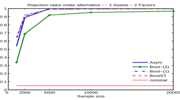
(26) since it can potentially rule out present and ‘easy’ to detect common conditionally heteroskedastic factor structures. The results for Designs 2 and 5 are displayed in Figures 4 and 5, respectively. Figure 4 shows that the standard bootstrap and the corrected bootstrap have similar power and this is slightly larger than the power associated with the use of critical values based on the fifty-fifty mixture of χ21 and χ22 . The continuously-corrected bootstrap has smaller power than these three tests, which is as expected given that it yields lower rejection rates under the null. In this case, where the true asymptotic distribution is known, the trade-off between power and size favors the asymptotic test based on the mixture of chi-square distributions. Nevertheless, this is no longer the case for Design 5, where the exact asymptotic null distribution is not known and the choice is between using the bootstrap or the conservative bound based on the χ23 distribution. Indeed, as Figure 5 shows, the latter approximation yields lower rejection rates under the alternative compared to the continuously-corrected bootstrap, which in turn is dominated by the standard bootstrap and the corrected bootstrap in terms of power. However, if we want to control the size of the test under the null and still achieve the largest possible power, the continuously-corrected bootstrap should be the preferred method.. 18.

(27) Rejection rates −− 2 Assets − 1 Factor 0.12 Asym Boot−(2) Boot−(1) BootST nominal. 0.11 0.1 0.09 0.08 0.07 0.06 0.05 0.04 0.03 0. 5000. 10000. 20000 Sample size. 40000. 50000. Figure 1: Rejection rates under the null for Design 1: JˆT ∼a 12 χ21 + 12 χ22 ; Rejection rates −− 3 Assets − 2 Factors 0.14 chi2−1 Boot−(2) Boot−(1) BootST chi2−3 nominal. 0.12. 0.1. 0.08. 0.06. 0.04. 0.02. 0. 0. 5000. 10000. 20000 Sample size. 40000. 50000. Figure 2: Rejection rates under the null for Design 3: JˆT ∼a minv J(v). Rejection rates −− 3 Assets − 1 Factor 0.07. 0.06. 0.05. 0.04. 0.03. chi2−1 Boot−(2) Boot−(1) BootST chi2−3 nominal. 0.02. 0.01. 0 0. 5000. 10000. 20000 Sample size. 40000. 50000. Figure 3: Rejection rates under the null for Design 4: asymptotic theory unavailable. 19.

(28) Rejection rates under alternative −− 2 Assets − 2 Factors 1 0.9 0.8 0.7 0.6 0.5 0.4 Asym Boot−(2) Boot−(1) BootST nominal. 0.3 0.2 0.1 0 0. 2000. 5000. 10000 Sample size. 20000. Figure 4: Rejection rates under the alternative for Design 2. Rejection rate under alternative −− 3 Assets − 3 Factors 1 0.9 0.8 0.7 0.6 0.5 0.4. chi2−1 Boot−(2) Boot−(1) BootST chi2−3 nominal. 0.3 0.2 0.1 0 0. 2000. 5000. 10000 Sample size. 20000. Figure 5: Rejection rates under the alternative for Design 5. 20.

(29) 6. Conclusions. The main contribution of this paper is to propose a new bootstrap method for GMM inference in the context of nonlinear overidentified models that are globally identified but not locally identified to first order. In particular, we focus on the special case of a degenerate rank identification condition, which was recently analyzed by Dovonon and Renault (2013) in the context of tests for common conditionally heteroskedastic factors. We show that the standard method of bootstrapping the overidentification test statistic as proposed by Hall and Horowitz (1996) fails under this condition. The main reason for the failure of the bootstrap is that the bootstrap moment conditions do not replicate the singularity of the Jacobian matrix present in the population. We offer an easy modification of the standard bootstrap method that consists of further recentering the bootstrap moment function by subtracting off a term that is proportional to the ˆ This second recentering of the bootstrap moment condition sample Jacobian matrix multiplied by θ−θ. ensures that the bootstrap Jacobian matrix is also degenerate in the bootstrap world, restoring the asymptotic validity of the bootstrap overidentification test.. Appendix A: Proof of results in Section 2 Proof of Proposition 2.1. The proof that θˆT − θ0 = oP (1) follows by Theorem 2.6 of Newey and McFadden (1994) under our Assumptions 1-3. Proof of Proposition 2.2. For part (i), we follow the proof of Proposition 3.1 of D&R (2013). The only difference is the fact that the moment conditions ψ considered here are not necessarily quadratic. ( ) ( ) For each h = 1, . . . , H, by a Taylor expansion of ψt,h θˆT ≡ ψh Xt , θˆT around θ0 , we have that (. ψt,h θˆT. ). ( ) 2ψ ¨ ( ) ( ) ) ∂ t,h θT ( ′ ∂ψt,h (θ0 ) ˆ 1 ˆ ˆ = ψt,h (θ0 ) + θ − θ + θ − θ θ − θ 0 0 0 , T T T ∂θ′ 2 ∂θ∂θ′. where θ¨T is a p×1 vector on the segment connecting θˆT and θ0 that may depend on h. The superscript (h) reflects the fact that the mean value may be different for each element ψt,h (θ) of ψt (θ). Stacking √ this equation over h = 1, . . . , H, summing over t and multiplying the result by T yields ( ) √ ) ( ) √ √ ∂ ψ¯T (θ0 ) ( ˆT − θ0 + 1 RT θ¨T , T ψ¯T θˆT = T ψ¯T (θ0 ) + T θ (5) ∂θ′ 2 ( ) where the remainder RT θ¨T is a H × 1 vector defined as (. RT θ¨T. ). ( )   ( )′ ∂ 2 ψ¯h,T θ¨T(h) ( ) √ θˆT − θ0  = T  θˆT − θ0 ∂θ∂θ′. . h=1,...,H. 21.

(30) For h = 1, . . . , H, we can write ( ) ( ) ′  (h) (( ( )′ ∂ 2 ψ¯h,T θ¨T(h) ( ) )( )′ ) ∂ 2 ψ¯h,T θ¨T ˆ ˆ ˆ ˆ   θT − θ0 θT − θ0 = vec vec θT − θ0 θT − θ0 , ∂θ∂θ′ ∂θ∂θ′ since tr (AB) = vec (A′ )′ vec (B). It follows that (( ( ) √ ( ) )( )′ ) ( ) ( ) ¯ θ¨T vec ¯ θ¨T vec vˆT vˆT′ , RT θ¨T = T G θˆT − θ0 θˆT − θ0 ≡G ( ) ) ( ¯ θ¨T is the random H × p2 matrix G ¯ (θ) defined in (4) evaluated where vˆT ≡ T 1/4 θˆT − θ0 and G ( ) ¯ θ¨T = G + oP (1) at θ¨T . Given our assumptions and the fact that θ¨T →P θ0 , we can show that G (see e.g. Lemmas 2.4 and 2.9 of Newey and McFadden (1994)). Thus, ( ) ( ) ( ) (h) RT θ¨T = Gvec vˆT vˆT′ + oP ∥ˆ vT ∥ 2 . This implies that ) ( ) ) ( √ √ √ ∂ ψ¯T (θ0 ) ( ( ) 2 ˆT − θ0 + 1 Gvec vˆT vˆ′ + oP ∥ˆ v ∥ T ψ¯T θˆT = T ψ¯T (θ0 ) + T θ T T ∂θ′ 2 ( ) √ ( ) 1 ′ ¯ = T ψT (θ0 ) + Gvec vˆT vˆT + oP (1) + oP ∥ˆ vT ∥2 , (6) 2 ) √ ¯T (θ0 ) ( ˆ where the oP (1) term is equal to T ∂ ψ∂θ θ − θ ′ 0 = OP (1) × oP (1) since under Assumption 6 T ( ¯ ) √ ¯T (θ0 ) T (θ0 ) (i), E ∂ ψ∂θ = 0 and thanks to Assumption 4(ii), therefore T ∂ ψ∂θ = OP (1) by a CLT applied ′ ′ { } ∂ψ(Xt ,θ0 ) to . It follows that ∂θ′ ( ) 1 vT vˆT′ )G′ WT Gvec(ˆ vT vˆT′ ) T ψ¯T′ (θˆT )WT ψ¯T θˆT = T ψ¯T′ (θ0 )WT ψ¯T (θ0 ) + vec′ (ˆ 4 √ +vec′ (ˆ vT vˆT′ )G′ WT T ψ¯T (θ0 ) + oP (1) + oP (∥ˆ vT ∥2 ) + oP (∥ˆ vT ∥4 ). The expected result follows from the same arguments as those used by D&R (2013) to prove their Proposition 3.1. The additional oP (∥ˆ vT ∥4 ) term that appears here does not alter the reasoning. We now establish (ii). Since ZT (θ0 ) = OP (1) and vˆT = OP (1), we have (vec′ (ZT (θ0 )) , vˆT′ )′ = OP (1). Therefore, from Prohorov’s theorem (see Theorem 2.4 of van der Vaart (1998)), the joint sequence has a subsequence that converges in distribution to (vec′ (Z(X)), V ′ )′ , say, where ) ( 2 ′ ∂ ρ (θ0 ) WX , Z(X) = ∂θi ∂θj 1≤i,j≤p and X ∼ N (0, Σ). Let “Z(X) ≥ 0” denote the event “Z(X) is positive semi-definite and “Z(X) ≥ 0” its complement. Under Assumption 6(ii), D&R (2013, Proposition 3.2) show that P (Z(X) ≥ 0) ≤ 1/2, which implies that P (Z(X) ≥ 0) ≥ 1/2 > 0. Since ( ) ( ) ( ) P (V ̸= 0) ≥ P V ̸= 0, Z (X) ≥ 0 = P V ̸= 0|Z (X) ≥ 0 P Z (X) ≥ 0 , it suffices to show that P (V = 0|Z(X) ≥ 0) = 0. To this end, we follow the proof of Proposition 22.

(31) 3.2 of D&R (2013). The second order necessary condition for an interior solution for a minimization problem implies that, for any unit vector e ∈ Rp , ( 2 ) ∂ ′ ′ ¯ ¯ e ψT (θ) WT ψT (θ) |θ=θˆT e ≥ 0, ∂θ∂θ′ which is equivalent to e′ (Z˜T + NT )e ≥ 0, with ( ( ) ( )) 2 √ ∂ ′ ¯ ˆ ¯ Z˜T = ψ θT WT T ψT θˆT , ∂θi ∂θj T 1≤i,j≤p. and NT =. ( ) √ ∂ ′ ( ) ∂ T ψ¯T θˆT WT ψ¯T θˆT . ∂θ ∂θ. The result follows exactly along the lines of the proof of D&R (2013) once we establish that ( ) ( ) 1 ∂ 2 ρ′ (θ0 ) ′ ˜ ZT = ZT (θ0 ) + W Gvec vˆT vˆT + oP (1), 2 ∂θi ∂θj 1≤i,j≤p and. ( ) 2 ′ ∂ 2 ρ (θ0 ) ′ ∂ ρ (θ0 ) NT = vˆT W vˆT + oP (1). ∂θi ∂θ ∂θj ∂θ′ 1≤i,j≤p. (7). (8). To show (7), we observe that from part (i), (6) implies that ( ) √ √ ( ) 1 ¯ T ψT θˆT = T ψ¯T (θ0 ) + Gvec vˆT vˆT′ + oP (1). 2. (9). P Given the dominance condition in Assumption 4 (i) and the fact that θˆT → θ0 , it follows that ( ) ∂ 2 ψ¯T′ θˆT ∂ 2 ρ′ (θ0 ) WT = W + oP (1), ∂θi ∂θj ∂θi ∂θj. which together with (9) implies (7). To obtain (8), by a mean-value expansion of. ∂ ψ¯T (θˆT ) ∂θi. around θ0 ,. we get that for all i = 1, . . . , p, ( ) ( ) ( ) 2¯ ∂ ψ¯T θˆT 2 ¯ ¯ 1/2 1/4 1/2 1/4 ∂ ψT (θ0 ) 1/2 ∂ ψT θ 1/4 ˆ 1/2 ∂ ρ (θ0 ) WT T = WT T +WT T θ − θ = W vˆT +oP (1) , 0 T ∂θi ∂θi ∂θi ∂θ′ ∂θi ∂θ′ where θ¯ ∈ (θ0 , θˆT ) and may differ from row to row. We obtain (8) by writing this equation for any i, j = 1, . . . , p and taking the inner product of each hand side. Proof of Theorem 2.1. We follow the proof of Lemma B.6 of D&R (2013). By a second-order mean √ value expansion of v 7→ T ψ¯T (θ0 + T −1/4 v) at 0, we have that ( ) √ √ ( ) ∂ ψ¯T 1 ¯ (¨ ) T ψ¯T θ0 + T −1/4 v = T ψ¯T (θ0 ) + T 1/4 ′ (θ0 ) v + G θ (v) vec vv ′ , ∂θ 2 ( ) where θ¨ (v) ∈ θ0 , θ0 + T −1/4 v and may differ from row to row. It follows that ( ) √ √ ( ) 1( ) 1 ¯ (θ0 ) − G vec(vv ′ ) T ψ¯T θ0 + T −1/4 v T ψ¯T (θ0 ) + Gvec vv ′ + G = 2 2 ) ( ) 1 ( ¯ (¨ ) ¯ ∂ ψ¯T + G θ (v) − G (θ0 ) vec vv ′ + T 1/4 ′ (θ0 ) v. 2 ∂θ Next, we show that the last three terms in the equation above are op (1) uniformly over any compact ¯ (θ0 ) − G = oP (1) and since subset K of Rp . Starting with the first of these terms, note that G 23.

(32) v ∈ K ⊂ Rp , this term converges to zero uniformly over K. For the term that follows, note that since ¨ ∈ N , a neighborhood of θ0 , θ0 is an interior point of Θ and K is compact (hence bounded), then θ(v) for all v ∈ K and T sufficientlty large. Hence, from Assumption 3(i), using the triangle inequality, the ( ) ( ) ¨ ¨ ¯ θ(v) ¯ 0 ), say G ¯ h θ(v) ¯ h (θ0 ) satisfies h-th row of G − G(θ −G T T ∑ ∑ ¨ − θ0 ∥ = 1 ¨ ¯ h (θ(v)) ¯ h (θ0 )∥ ≤ 1 m(Xt )∥θ(v) m(Xt )(1 − α)T −1/4 ∥v∥, ∥G −G T T t=1. t=1. ¯. ψT for some 0 ≤ α ≤ 1. Thus, this term is oP (1) uniformly over K. Finally, note that ∂∂θ ′ (θ0 ) = ( ) ( −1/2 ) ∂ψt OP T by a CLT since E ∂θ′ (θ0 ) = 0. This implies that the last term is also oP (1) uniformly. over K. As a result, √. ¯ 0 + T −1/4 v) = T ψ(θ. √ 1 T ψ¯T (θ0 ) + Gvec(vv ′ ) + oP (1), 2. implying that √ √ √ 1 JT (v) = T ψ¯T′ (θ0 )W T ψ¯T (θ0 ) + vec′ (vv ′ )G′ W T ψ¯T (θ0 ) + vec′ (vv ′ )G′ W Gvec(vv ′ ) + oP (1), 4 where the neglected terms are uniformly (asymptotically) negligible over any compact subset K. Since this is the analogue of equation (B.4) of D&R (2013), the rest of the proof follows exactly the same lines as the proof of Lemma B.6 of D&R (2013). To complete the proof of Theorem 2.1, we show that the random variable J ≡ minv∈Rp J(v) has a continuous distribution. We adopt the notation J(X, v) for J(v) to highlight its dependence on X which is its only source of randomness. We show that ∀c ∈ R, that. Prob(J = c) = 0. It is easy to see. )′ ( ) ( 1 1 ′ ′ J(X, v) = X + Gvec(vv ) W X + Gvec(vv ) . 2 2. Since W is symmetric positive definite, J(x, v) ≥ 0, c) = 0,. ∀x ∈ RH and v ∈ Rp . As a result, Prob(J =. ∀c < 0.. We show next that J cannot have an atom of probability at any c > 0. Let us assume by contradiction that there exists c∗ > 0 such that Prob(J = c∗ ) > 0. Let { } H ∗ A = x ∈ R : minp J(x, v) = c . v∈R. By definition, Prob(X ∈ A) = Prob(J = c∗ ) > 0. As a result, since the distribution of X is absolutely continuous with respect to the Lebesgue measure on RH , A contains an open ball centered at a certain x0 ∈ RH , say B(x0 , ϵ) = {x ∈ RH : ∀d ∈. RH. :. ∥d∥ < ϵ,. ∥x − x0 ∥ < ϵ} for some ϵ > 0. This implies that. minv∈Rp J(x0 + d, v) = c∗ . Let v0 ∈ arg minv∈Rp J(x0 , v) (such an argmin. exists for almost every x0 ∈ RH by D&R’s (2013) Lemma B6(ii)). Since x0 ∈ A, J(x0 , v0 ) = c∗ and ∀d ∈ RH :. ∥d∥ < ϵ, we have that. J (x0 , v0 ) = minp J(x0 + d, v) ≤ J(x0 + d, v0 ) = J(x0 , v0 ) + 2d′ W x0 + d′ W d + d′ W vec(v0 v0′ ). v∈R. 24.

(33) (The second equality above is obtained by expanding the expression of J(x0 + d, v0 ).) That is, ( ) 1 1 ′ ′ 2d W (x0 + Gvec(v0 v0 )) + W d ≥ 0, ∀d ∈ B(0, ϵ). 2 2. (10). Note that since J(x0 , v0 ) = c∗ = a′ W −1 a > 0, we must have a ≡ W (x0 + 12 GV ec(v0 v0′ )) ̸= 0. Fix aj ̸= 0, the j th element of a that is different from zero. Equation (10) implies that if we choose d with all entries equal to zero except dj such that −ϵ < dj < ϵ, then dj (2aj + Wjj dj ) ≥ 0 for all such dj . Since Wjj > 0, dj (2aj + Wjj dj ) = 0 has two roots, 0 and −2aj /Wjj ̸= 0. It follows that the sign of the polynomial dj (2aj + Wjj dj ) must change in a neigborhood of zero, implying that it is impossible to have dj (2aj + Wjj dj ) ≥ 0 for all −ϵ < dj < ϵ. Thus, it must be that Prob(J = c∗ ) = 0 for any c∗ > 0. To complete the proof, we need to show that J does not have an atom of probability at 0. To this end, we show that there exists a random variable L that is such that 0 ≤ L ≤ J and Prob(L = 0) = 0. ( )′ ( ) Let L = minu∈Rp2 X + 12 Gu W X + 21 Gu . Clearly, L ≤ J. Assume that Rank(G) = r. Given the second-order identification condition, G ̸= 0 and r > 0. Consider a rank factorization of G: G = G1 G2 , where G1 is H × r and G2 is r × p2 , both of rank r. The first order condition associated with L solved at u ˆ implies that G2 u ˆ = −2(G′1 W G1 )−1 G′1 W X. Consequently, we can write ( )′ ( ) 1 1 L = X + G1 G2 u ˆ W X + G1 G2 u ˆ = X ′ W 1/2 P W 1/2 X, 2 2. (11). where P = IH − W 1/2 G1 (G′1 W G1 )−1 G′1 W 1/2 is the orthogonal projection matrix on the subspace of dimension H − r that is orthogonal to the space spanned by the columns of W 1/2 G1 . Hence, there exists an H × H matrix Q such that Q′ Q = IH and P = Q′ DQ, where D = diag (IH−r , 0). Thus, L = Y ′ DY , with Y = QW 1/2 X ∼ N (0, S) and S = QW 1/2 ΣW 1/2 Q′ positive definite. Hence, ∑ 2 L = H−r i=1 Yi . Clearly, Prob(L = 0) ≤ Prob(Y1 = 0) = 0. This concludes the proof.. Appendix B: Proofs of results in Section 3 and 4 .1. Preliminaries. A convenient way to formalize the bootstrap is as follows (see Gon¸calves and White (2004) for a similar framework). Given the underlying probability space (Ω, F, P ), we observe a sample of size T , XT ≡ {X1 (ω) , X2 (ω) , . . . , XT (ω)} from a given realization ω ∈ Ω. Suppose we obtain a bootstrap sample XT∗ = {X1∗ , X2∗ , . . . , XT∗ } by resampling from XT . For each ω ∈ Ω, we view {Xt∗ : t = 1, . . . , T } as the realization of a stochastic process defined on (Λ, G, P ∗ ) , another probability space, such that for each t = 1, . . . , T, Xt∗ (ω, λ) = Xτt (λ) (ω) ,. (12). where τt : Λ → {1, 2, . . . , N } denotes the random index generated by the resampling scheme for each t = 1, 2, . . . , T (independently of ω). Thus, P ∗ describes the probability of bootstrap random variables, conditional on the observed data XT , i.e. P ∗ describes the probability induced by λ, conditional on ω.. 25.