3D Numerical Modeling of Transient Conditions in Francis Turbines

(1)

UNIVERSITÉ DE MONTRÉAL

3D NUMERICAL MODELING OF TRANSIENT CONDITIONS IN FRANCIS TURBINES

HOSSEIN HOSSEINIMANESH DÉPARTEMENT DE GÉNIE MÉCANIQUE ÉCOLE POLYTECHNIQUE DE MONTRÉAL

THÈSE PRÉSENTÉE EN VUE DE L’OBTENTION DU DIPLÔME DE PHILOSOPHIAE DOCTOR

(GÉNIE MÉCANIQUE) AVRIL 2016

(2)

UNIVERSITÉ DE MONTRÉAL

ÉCOLE POLYTECHNIQUE DE MONTRÉAL

Cette thèse intitulée :

3D NUMERICAL MODELING OF TRANSIENT CONDITIONS IN FRANCIS TURBINES

présentée par : HOSSEINIMANESH Hossein

en vue de l’obtention du diplôme de : Philosophiae Doctor a été dûment acceptée par le jury d’examen constitué de :

M. VO Huu Duc, Ph. D., président

M. REGGIO Marcelo, Ph. D., membre et directeur de recherche M. GUIBAULT François, Ph. D., membre et codirecteur de recherche M. TRÉPANIER Jean-Yves, Ph. D., membre

(3)

DEDICATION

(4)

ACKNOWLEDGEMENTS

I would like to take this opportunity to express sincere gratitude to my supervisors, Professor Francois Guibault and Professor Marcello Reggio for their excellent guidance, caring, patience, suggestions and availability during my research.

I gratefully acknowledge Dr. Christophe Devals for his support and share valuable expertise from the initial to the final level of the project. I would also thank Dr. Julien Dompierre and Dr. Marie-Gabrielle Vallet for providing valuable comments and suggestions.

I would like to thank Andritz Hydro Canada Inc. for their supports for the project. I also deeply appreciate members of R&D division: Mr. Vu, Mr. Nennemann for their excellent guidance and instructive comments during the research work.

The financial support of NSERC for this research is acknowledged.

A great thank you goes to my colleagues and teammates at Ecole Polytechnique for their valuable emotional and technical supports during the completion of the project.

Finally, I would like to thank with deepest gratitude to my father and mother who provided unconditional supports and encouragements throughout my life. I would also like to acknowledge my brother and sister for their supports.

(5)

RÉSUMÉ

Ces dernières années, plusieurs études se sont intéressées à l'amélioration de la conception des turbines hydroélectrique dans le but de réduire les effets négatifs des conditions d'opération hors design et des phénomènes transitoires. Néanmoins, encore plus d'efforts sont nécessaires pour fournir aux ingénieurs de conception des méthodes de simulation efficaces et robustes pour des conditions d'exploitation complexes et instationnaires. Il existe plusieurs approches concurrentes en cours de développement qui doivent être évaluées et comparées. Cette recherche vise à combler ce manque, en développant et en évaluant des méthodologies d'analyse des turbines Francis lors des opérations de rejet de charge, de vitesse à vide et d'emballement.

Cette recherche évalue des techniques de calcul de la vitesse d'emballement et de la vitesse à vide en utilisant des simulations numériques stationnaires et instationnaires. Deux méthodes sont comparées en calculant des paramètres dynamiques de la turbine pour trois cas composés de turbines Francis de haute et moyenne chute. Les simulations en stationnaire sont faites en utilisant un résoluteur fluide commercial, couplé avec un algorithme itératif basé sur la relation entre le couple de la roue et la vitesse. Toutes les simulations stationnaires sont faites sur un seul passage du distributeur et de la roue, connectés avec un modèle d'interface de mélange. Pour la seconde méthode, les simulations instationnaires, utilisant la moyenne de Reynolds des équations de Navier-Stokes (RANS), sont couplées à une sous-routine maison qui calcule et retourne le pas de temps, la vitesse de rotation de la roue et le couple de frottement. Les simulations instationnaires sont effectuées sur deux configurations géométriques: une turbine complète et sur un seul passage du distributeur et de la roue. Le modèle de rotor-stator transitoire (TRS) est utilisé pour coupler le distributeur avec la roue, et la roue avec l'aspirateur, dans le cas de la turbine complète. Un modèle d'interface de mélange est utilisé coupler un passage du distributeur avec un passage de la roue, et un passage de la roue avec l'aspirateur. Les simulations instationnaires avec le modèle TRS sont plus précises que les simulations stationnaires et instationnaires avec le modèle d'interface de mélange, pour calculer la vitesse d'emballement et la vitesse à vide pour plusieurs angles d'ouverture. Les simulations stationnaires fournissent un compromis entre la précision et l'effort de calcul nécessaire pour calculer les vitesses d'emballement et à vide.

(6)

Dans la deuxième partie du projet, les simulations instationnaires sont utilisées avec succès pour étudier le fonctionnement sans charge d'une turbine Francis. La simulation numérique d'un écoulement fluide est difficile parce que l'écoulement est irrégulier et instable à cause de la présence de décollements de l’écoulement, de formation de tourbillons, et d'oscillations de large amplitude de la pression dans la roue et l'aspirateur. Ces simulations permettent une meilleure compréhension de la physique de l'écoulement et des fluctuations de la pression dans la roue et l'aspirateur. On observe que les simulations instationnaires avec une interface de mélange ne sont pas capables de prédire les détails relatifs aux fluctuations du couple et de la pression durant les phénomènes transitoires. En outre, les résultats des simulations montrent une différence significative dans le calcul de la pression sur les pales entre les simulations instationnaires avec le modèle TRS et le modèle d'interface de mélange. Le principal défi des simulations instationnaires avec le modèle TRS est son très grand coût de calcul.

Enfin, l'objectif principal de cette thèse est atteint par l'élaboration et la validation d'une méthode basée sur la CFD pour prédire le comportement d'une turbine Francis dans le cas du rejet de charge. La méthodologie utilisée pour modéliser le rejet de charge est une extension de celle utilisée pour modéliser l'emballement et la vitesse à vide. Le principal défi de simulation provient de la rotation des directrices et est résolu avec la déformation de maillage et le remaillage. La variation de la vitesse de la roue est calculée en utilisant une équation du moment angulaire mis en œuvre dans une fonction définie par l'utilisateur. La méthodologie proposée a été élaborée en effectuant des simulations 2D instationnaires sur le modèle de turbine Francis de haute chute utilisé dans le workshop Francis-99, et validé par des simulations instationnaires 3D sur une turbine Francis de moyenne chute. Ces simulations permettent le calcul de paramètres d'ingénierie tels que la vitesse angulaire de la roue, la physique de l'écoulement et la charge sur les pales durant le rejet de charge. La validation des résultats numériques avec les résultats expérimentaux montrent un écart de 9% dans la prédiction de la vitesse maximale atteinte par la roue pendant le rejet de la charge. L'étude de l'écoulement relève la présence de structures complexes tels que le flux inversé, ou de pompage, à proximité du centre du diffuseur conique, et un flux tangentiel vers le bas près de la paroi du diffuseur conique. Des fluctuations de pression sont observées lorsque le point d'opération de la turbine Francis traverse les conditions de couple négatif. La méthodologie proposée présente une analyse qualitative de la physique de l'écoulement et du comportement de la turbine en cas de rejet de charge. Des mesures de la

(7)

pression sur la pale durant le rejet de charge sont calculées et validées. Une forte pression au bord d'attaque est prédite par les simulations numériques et est observée dans les résultats expérimentaux.

Pour conclure, les méthodologies proposées utilisant des simulations instationnaires de l'emballement, prédisent avec succès l'évolution des quantités d'ingénierie telles que la vitesse de rotation et le couple, ce qui peut contribuer au design de turbines dans ces conditions transitoires. En outre, une meilleure compréhension des phénomènes complexes à l'intérieur de la turbine est obtenue pour le rejet de charge et l'emballement.

(8)

ABSTRACT

In recent years, several studies have focused on improving hydroelectric turbine designs in order to decrease the negative influence of off-design conditions and transient processes. Nevertheless, greater effort is still needed to provide design engineers with efficient and robust simulation methodologies for complex unsteady operating condition. There are several competing approaches currently in development that must be evaluated and compared. This study aimed to reduce this gap in the research, by evaluating and developing methodologies for analyzing Francis turbine operations during load rejection, no-load condition, and runaway.

The research evaluated techniques for the calculation of the runaway speed, and no-load speed using steady and unsteady simulations. Two methods were compared by calculating turbine dynamic parameters for three test cases, consisting of high and medium head Francis turbines. The steady simulations were conducted using a commercial flow solver, and an iterative algorithm based on the relation between runner torque and speed. All steady simulations were performed on a single runner/distributor passage connected through a stage interface model. In the second method, unsteady RANS simulations were integrated with a user subroutine, to compute and return the value of the runner speed, the time step, and the friction torque. The unsteady simulations were performed for two geometric configurations: the complete turbine, and a single runner/distributor passage. The transient-rotor stator (TRS) model was used for connecting the runner and distributor, and the runner and draft tube in the complete turbine. The stage interface model was used for connecting the runner and distributor passages, and the runner’s passage and draft tube. The unsteady simulations using TRS model were found more accurate than the steady and unsteady stage simulations for calculating the runaway and no-load speed for many opening angles. The steady simulations provided a compromise between accuracy and the computational effort required to calculate the runaway and no-load speed. In the second part of the project, the unsteady simulations were successfully applied in order to investigate the operation of a Francis turbine at no-load conditions. Numerical flow simulation was challenging, because the flow was irregular and unstable owing to large flow separation, vortex formation, and large amplitude pressure oscillations in the turbine and draft tube. The simulations led to a deeper understanding of flow physics and pressure fluctuations in the turbine and draft tube. It was observed that the unsteady simulations with stage interface model were not

(9)

capable of predicting details pertaining to fluctuations of the torque and pressure during transient processes. Moreover, the simulation results showed the sizeable difference in computing the pressure on the blades between the unsteady simulations with TRS and stage interface models. The main challenge of unsteady simulations with the TRS model was dependency on more expensive computational costs.

Finally, the main objective of this thesis was achieved by developing and validating a methodology to predict the operation of a Francis turbine during load rejection, based on CFD simulations. The methodology for the runaway and no-load simulation was extended for modelling the load rejection. Mesh deformation and re-meshing techniques were used to address the simulation challenges caused by the guide vane rotation. The runner speed variation was computed using an angular momentum equation, implemented in a user defined function. The proposed methodology was developed by performing 2D unsteady simulations on a high head model Francis turbine used in the Francis-99 workshop, and validated by 3D unsteady simulations on a medium head Francis turbine. These simulations allowed the computing of the engineering quantities such as turbine angular speed, flow physics, and unsteady load on blades during the process. The validation of CFD results with experiments showed 9% discrepancy in the prediction of the maximum speed attained by turbine during the load rejection. The investigation of flow physics revealed the presence of complex flow structures such as reversed flow (pumping flow) near the draft tube cone center, and a downward tangential flow near the cone wall of the draft tube. Pressure fluctuations were captured when the Francis turbine’s operating point moves through conditions of negative torque. The proposed methodology presented a qualitative analysis of the flow physics, and turbine behavior during load rejection. The pressure signals on the blade were evaluated, and validated during load rejection. Strong pressure signals were predicted at the leading edge for CFD and observed in the experiments. To conclude, the proposed methodologies using unsteady simulations successfully predicted the evolution of engineering quantities such as the rotational speed and torque during the runaway process, which could contribute in designing turbine considering the transient behaviors. Moreover, the better insights of complex phenomena inside the turbine were obtained during load rejection and runaway processes.

(10)

LIST OF TABLES

Table 2-1 Literature review of CFD simulations of hydraulic turbines during transient processes

... 17

Table 4-1: Test case specifications. ... 27

Table 4-2: Number of nodes for simulation domains. ... 27

Table 4-3 : Maximum discrepancy between the numerical and experimental speed factors. ... 38

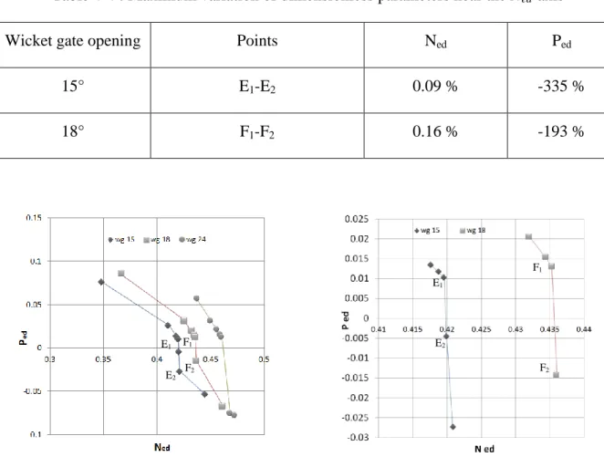
Table 4-4 : Maximum variation of dimensionless parameters near the Ned-axis. ... 44

Table 5-1 : Turbine geometry and mesh specifications used in no-load simulations ... 56

Table 5-2 : Average Y+ for simulation domains. ... 61

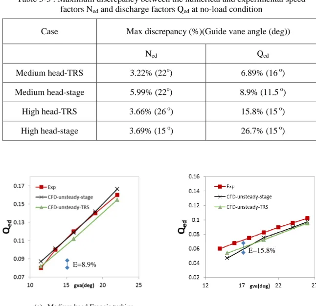
Table 5-3 : Maximum discrepancy between the numerical and experimental speed factors Ned and discharge factors Qed at no-load condition ... 69

Table 5-4 : Comparison of normalized averaged pressure fluctuations in BEP and no-load condition for medium head-TRS & stage simulations at gva 16°.(PS: blade pressure side, SS: blade suction side) ... 70

Table 5-5 : Comparison of averaged and maximum pressure at no-load between medium head-TRS & stage simulations for a gva 16°. ... 80

Table 6-1: Turbine specifications at load rejection simulations. ... 90

Table 7-1 : Comparison of typical no-load simulations of a high head Francis turbine launched on a high performance computer (HPC) platform. ... 109

(15)

LIST OF FIGURES

Figure 1-1: Schematic diagram of a hydroelectric power plant ... 1

Figure 1-2: Operation areas of hydro turbines(Wagner et al., 2011) ... 3

Figure 1-3: Cross-section view of a Francis turbine installation (Round, 2004) ... 3

Figure 1-4: Side view of a typical Francis turbine layout (Round, 2004) ... 4

Figure 4-1: Mesh for components for test case 1: (a) distributor passage, stay vane and guide vane, (b) runner passage, (c) draft tube. ... 28

Figure 4-2: Geometry and boundary conditions of computational domains (test case 1). ... 29

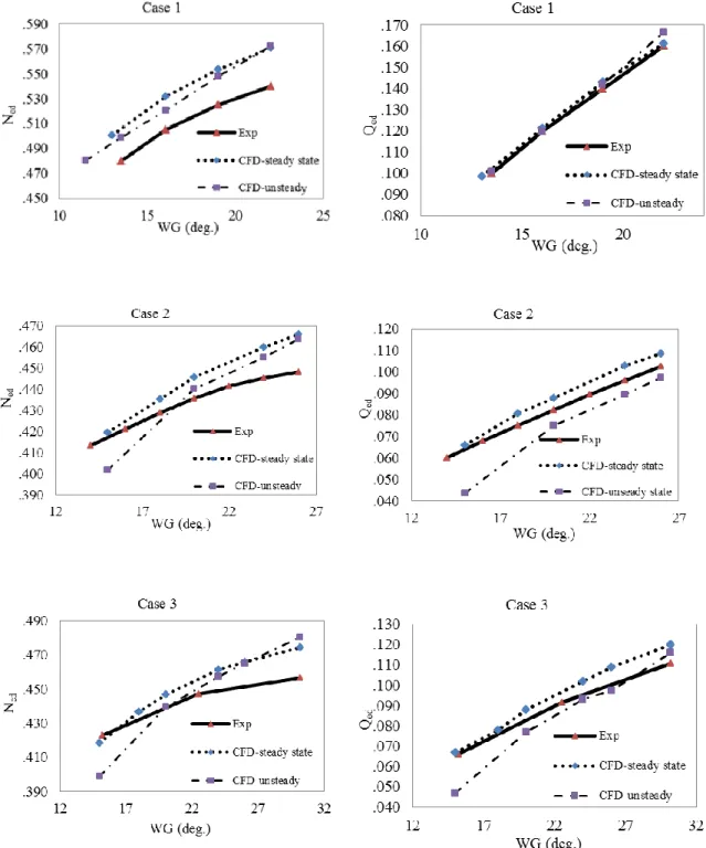
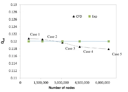
Figure 4-3 : Speed factor Ned & discharge factor Qed vs. wicket gate angles (WG) from CFD and experiments at no-load speed. ... 39

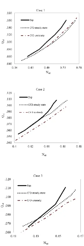
Figure 4-4: No-load speed line computed from CFD and experiments. ... 40

Figure 4-5 : Normalized axial velocity field, velocity vectors and streamlines on a section plane crossing the draft tube in steady (left) and unsteady (right) simulations at wicket gate angle of 15 degrees case 2 ... 41

Figure 4-6 : Comparison time-averaged normalized velocity field and 2D streamlines between steady (left) and unsteady (right) simulations at wicket gate angle of 15 degrees at 1% span case 2 ... 42

Figure 4-7 : Comparison time-averaged normalized velocity field and 2D streamlines between steady (left) and unsteady (right) simulations at wicket gate angle of 15 degrees at 50% span case 2 ... 42

Figure 4-8 : Power factor Ped vs. speed factor Ned for test case 2 in steady simulations. ... 44

Figure 4-9 : Speed factor Ned vs dimensionless accumulated time step t* by steady and unsteady methods ... 45

Figure 4-10 : Speed factor Ned vs dimensionless accumulated time step t* by unsteady method .. 46

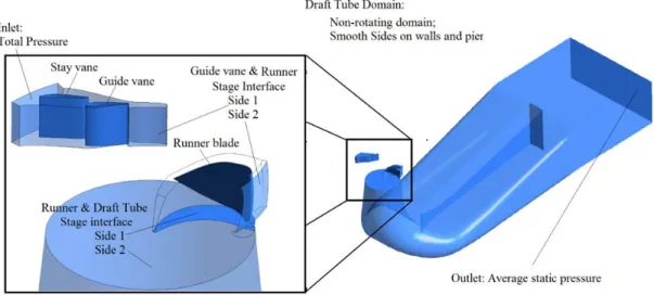
Figure 5-1 : Mesh for Francis turbine & distributor (left), computational domain of complete turbine in medium head-TRS simulation (right). ... 55

(16)

Figure 5-2 : Mesh for components in medium head-stage simulation: (a) distributor passage, stay vane and guide vane, (b) runner passage, (c) draft tube. ... 55 Figure 5-3 : Mesh quality histograms (a) Element volume (log value) distribution, ( b) Minimum

angle distribution,(c) Expansion factor distribution ... 58 Figure 5-4 : Comparison of simulated and experimental discharge factor Ned at no-load condition

for different mesh densities. ... 59 Figure 5-5 : Comparison of simulated and experimental discharge factor Qed at no-load condition

for different mesh densities ... 59 Figure 5-6 : Distribution of Y+ at no-load on medium head Francis turbine components (gva 16°) ... 62 Figure 5-7 : Geometry and boundary conditions of computational domains in medium head-stage

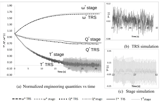
simulation. ... 63 Figure 5-8 : Variation of the normalized runner angular speed, flow rate, torque in medium head-TRS & stage simulations for a gva 16° ... 67 Figure 5-9 : Comparison between CFD predictions and experimental measurements (ANDRITZ

Hydro, 2014) of speed coefficients Ned at no-load conditions (E=Error bar) ... 68 Figure 5-10 : Comparison between CFD predictions and experimental measurements (ANDRITZ

Hydro, 2014) of flow coefficients Qed at no-load conditions (E= Error bar) ... 69 Figure 5-11 : Monitoring points on pressure (PS) and suction (SS) sides of blade in medium

head-TRS & stage simulations ... 70 Figure 5-12 : Time history of normalized pressure fluctuation at PS and SS in medium head-TRS

& stage simulations for a gva 16° ... 71 Figure 5-13 : Spectral analysis of normalized pressure fluctuations at SS & PS at no-load from

medium head-TRS & stage simulations for a gva 16° ... 72 Figure 5-14 : Normalized time-averaged pressure distribution on the blade pressure (left) and

suction (right) sides at BEP (top) and no-load (bottom) from medium head-TRS simulation for a gva 16° ... 73

(17)

Figure 5-15 : 3D Streamlines of normalized time-averaged velocity within runner at no-load in medium head-TRS simulation for a gva 16° ... 74 Figure 5-16 : Normalized time-averaged axial vorticity at 1% span (left) and 50% span (right)

runner at no-load from medium head-TRS simulation for a gva 16°... 75 Figure 5-17 : Normalized time-averaged velocity streamlines & vorticity magnitude at mid

surface in blade channel at no-load condition from medium head-TRS simulation for a gva 16°. ... 75 Figure 5-18 : Normalized time-averaged tangential velocity (left) and axial velocity field (right)

on a plane section through the draft tube at no-load from medium head-TRS simulation for a gva 16°... 76 Figure 5-19 : Comparison of time-average pressure coefficient Cp at no-load from medium

head-TRS & stage simulations for a gva 16° at different spans ... 77 Figure 5-20 : Comparison of normalized time-averaged velocity field and 2D velocity streamlines

at no-load condition between medium head-TRS (left) and medium head-stage (right) simulations for a gva 16° on the plane z/L = -0.4 crossing the runner ... 78 Figure 5-21 : Comparison of normalized time-averaged pressure distribution on the blade suction

side at no-load condition between medium head-TRS (left) and medium head-stage (right) simulations for a gva 16° ... 79 Figure 5-22 : Comparison of normalized time-averaged pressure distribution on the blade

pressure side at no-load condition between medium head-TRS (left) and medium head-stage (right) simulations for a gva 16° ... 79 Figure 5-23 : Comparison of normalized time-averaged velocity field and 2D velocity streamlines

at no-load condition between medium head-TRS (left) and medium head-stage (right) simulations for a gva 16° at a plane crossing the draft tube ... 81 Figure 6-1: Computational domain of high head model Francis turbine (Francis-99) in 2D

unsteady simulations. ... 89 Figure 6-2: Geometry and boundary conditions of computational domains in 3D-medium head

(18)

Figure 6-3 : Wicket gate closing scenario for 3D medium head Francis simulations. ... 92 Figure 6-4 : Schematic illustration of the wicket gate closing simulation ... 93 Figure 6-5 : Mesh motion conditions of the wicket gate passage ... 94 Figure 6-6 : Variation of the normalized runner angular speed in 3D medium head simulations

and experiment. ... 96 Figure 6-7 : Variation of the normalized runner torque and flow rate during load rejection in 3D

medium head simulation. ... 96 Figure 6-8: Monitoring points on pressure (PS) and suction (SS) sides of blade in medium head-TRS & stage simulations. ... 97 Figure 6-9: Time history of normalized pressure at monitoring points on the pressure side. ... 98 Figure 6-10: Time history of normalized pressure at monitoring points on the suction side. ... 98 Figure 6-11: Spectral analysis of normalized pressure fluctuation at monitoring points on the

pressure side (fn: frequency of runner rotation at best efficiency operating point). ... 100

Figure 6-12: Spectral analysis of normalized pressure fluctuation at monitoring points on the suction side (fn: frequency of runner rotation at best efficiency operating point). ... 100

Figure 6-13: Evolution of normalized pressure distribution on the blade pressure (left) and suction (right) sides during load rejection from 3D medium head simulation ... 101 Figure 6-14 : Evolution of normalized swirl at draft tube inlet during load rejection simulation. ... 102 Figure 6-15: Normalized tangential velocity field on a cross section through the draft tube during

load-rejection from 3D medium head simulation. ... 103 Figure 6-16: Normalized axial velocity field on a cross section through the draft tube at no-load

from 3D medium head simulation. ... 103 Figure 7-1: Evolution of dimensionless speed and torque during no-load simulation of a medium

head Francis turbine at gva 16º. ... 110 Figure 7-2 : Evolution of friction and turbine torque at the end of the runaway simulation for the

(19)

Figure 7-3 : Time history of normalized pressure fluctuation in medium head-Francis turbine during load-rejection (left) and at no-load condition (right). ... 113 Figure 7-4 : Evolution of the runner’s speed during load rejection and no-load simulations at the

(20)

LIST OF SYMBOLS AND ABBREVIATIONS

BEP Best efficiency operating point 𝐶_𝑚 Torque coefficient (= 0.0311 (_𝑅𝑒1 10.2) ( 𝑟ℎ𝑢𝑏 𝐺𝐴𝑃𝐶) 0.1 ) 𝐶𝑛 torque coefficient (= 0.065(_𝑟̅𝐺𝑎𝑝 𝑠ℎ𝑟𝑜𝑢𝑑) 0.3_(𝑅𝑒)−0.2₎ 𝐶_𝑃 pressure coefficient (=𝑃−𝑃𝑎𝑡𝑚1 2𝜌𝑉𝑏𝑙𝑑𝑡2 ) 𝐶𝜀1 constant number (=1.44) 𝐶𝜀2 constant number (=1.92) 𝐶_𝜇 constant number (=0.09) 𝐷 or 𝐷_ℎ turbine throat diameter, m F body force of unit mass fluid, N

E hydraulic energy

f frequency, Hz

fn turbine frequency at BEP, Hz

g gravitational Acceleration, m/s2 gva guide vane angle (degree)

H turbine net head, m

𝐼_𝑧 moment of inertia of the runner, kg m2 K turbulent kinetic energy (= 1₂√𝑢̅̅̅̅̅) _𝑖,𝑢_𝑖, L height of distributor passage, m 𝑙_𝑖 shroud seal length, m

(21)

N turbine rotational speed, rpm

Ned speed factor, Energy Units (= _{60√𝑔𝐻}𝑁𝐷 )

P pressure, N/m2

𝑃_𝑎𝑡𝑚 atmospheric pressure, Pa Ped,n power factor at n iteration,

𝑃_𝑟𝑒𝑓 reference pressure, Pa (= 𝜌𝑔𝐻 ) 𝑃𝑒𝑑 ,𝑛 average of power factor at n-5 cycles

P* normalized pressure (= 𝑃 𝑃⁄ 𝑟𝑒𝑓)

Q discharge, m3/s

Qed discharge factor (= _𝐷₂_√𝑔𝐻𝑄 )

Q* normalized discharge (Q/QBEP)

𝑟_ℎ𝑢𝑏 runner leading edge radius at the hub, m 𝑟̅𝑠ℎ𝑟𝑜𝑢𝑑 average shroud radius, m

Re Reynolds number (=𝜋𝑁𝐷_ℎ2_/60)

Re₁ Reynolds number (=𝜔𝜌𝑟 ℎ𝑢𝑏2

𝜇 )

Re2 Couette Reynolds number (= 𝜌𝜔𝐺𝑎𝑝𝑟̅_𝜇𝑠ℎ𝑟𝑜𝑢𝑑)

t time, sec

𝑡_{𝐺𝑎𝑝 𝑠ℎ𝑟𝑜𝑢𝑑} width of the runner shroud clearance, m 𝑡_{𝐺𝑎𝑝 ℎ𝑢𝑏} runner hub clearance, m

𝑡∗ _{dimensionless accumulated time step}

T or Tn hydraulic force torque, Nm (= 𝑇𝑟(𝑡) − 𝑇𝑓𝑟(𝑡))

(22)

𝑇_𝑓𝑟 friction torques on turbine hub and shroud, Nm (= 𝑇_{𝑓𝑟,ℎ𝑢𝑏} + 𝑇_{𝑓𝑟,𝑠ℎ𝑟𝑜𝑢𝑑}) 𝑇𝑓𝑟,ℎ𝑢𝑏 friction torques on hub, Nm (= 𝐶𝑚𝜌𝜔

2_𝑟 ℎ𝑢𝑏5

2 )

𝑇_{𝑓𝑟,𝑠ℎ𝑟𝑜𝑢𝑑} friction torque on shroud, Nm (= 𝐶𝑛𝜌𝜋𝜔2𝑟̅𝑠ℎ𝑟𝑜𝑢𝑑4 ∙𝑙𝑖

2 )

𝑇𝑔 torque of the electromagnet, Nm

𝑇_𝑟 torque of the pressure and viscous forces on runner blade, Nm

V velocity, m/s

𝑉_{𝑏𝑙𝑑𝑡} average flow velocity on blade draft tube interface, m/s 𝑉_𝑟𝑒𝑓 reference velocity, m/s (= √𝑔𝐻 )

V* normalized velocity (= 𝑉 𝑉⁄ 𝑟𝑒𝑓)

 fluid density, kg/m3

𝜌𝑢̅̅̅̅̅ _𝑖,𝑢_𝑗, Reynolds shear stress, N/m2 𝛿𝑖𝑗 Kronecker delta

𝜎𝑘 constant number (=1.0)

𝜔 runner angular speed, rad/sec 𝜔∗ _{normalized angular speed (ω/ω}

BEP)

𝜎_𝜀 constant number (=1.3) 𝜇_𝑡 turbulent viscosity, N s/m2

𝜇 dynamic viscosity of water, N s/m2 wga wicket gate angle (degree)

(23)

CHAPTER 1 INTRODUCTION

1.1 Hydropower

According to Renewables Global Status Report (GSR) (Ren, 2015), hydroelectric power provided an estimated 16.6% of the global electricity demand, and about 73% of the electricity from renewable sources. With virtually no output of greenhouse gas compared to fossil fuels, no direct waste and lower safety risk in comparison to nuclear power plants, hydroelectric power appears to be one of the most ecologically-friendly sources to meet the growing energy demand.

Hydroelectric power plants are composed of four main parts: the turbine, electric generator, transformer as well as upper and lower reservoirs. Figure 1-1 illustrates a schematic diagram of a hydroelectric power plant. Basically the flow passes through the penstock from the reservoir to reach the turbine which converts the energy in the water into mechanical power through a rotating shaft. Then the rotation of the shaft is converted into electric power by the electric generator. A series of rotating coils inside a magnetic field produces the electrical current. Finally the transformer increases the voltage of the electrical current before transmitting the power to the grid.

Figure 1-1: Schematic diagram of a hydroelectric power plant

1.2 Hydroelectric turbines operation

Hydroelectric turbines are synchronous machines, which implies that all the energy extracted from the water must immediately be consumed on the network. Therefore, the electric load on the generator must always balance the power mechanically extracted from the water. In case of slight

Generato Upper reservoir Lower reservoir Dam Penstock Turbine Draft tube Tailrace Inlet Transformer Power House

(24)

perturbations on the load, the turbine governor system will adjust the mass flow rate to compensate for the variations. However, in case of a complete drop or absence of load, the turbine cannot be suddenly stopped. Otherwise, the entire system may experience severe and extreme pressure fluctuations called water hammer, which may seriously damage and even destroy the turbine (Seleznev et al., 2014).

The turbine may be identified as the heart of the hydropower plants because of its role for developing torque from the dynamic action of water. This important part can be classified based on pressure change of water into two types: the impulse turbine, such as the Pelton turbine, which uses a high speed jet for converting kinetic energy of the fluid into revolving movement of the shaft while the pressure of the fluid doesn’t change in this condition. The second type is called the reaction turbine, because the reaction of the fluid on the turbine blades produces the power through variation of velocity and pressure.

Two important types of reaction turbines are the Francis and the Kaplan. In the Kaplan turbine, the passing flow is in direction of axis of the rotation. But the flow inside a Francis turbine comes in the radial direction and leaves in the axial direction. Hence the Francis turbine is called as mixed flow turbine.

Additionally these types of turbines can be selected for different operation conditions (see Figure 1-2). Basically the Pelton turbine operates at low discharge and high head. The Francis turbine is appropriate for medium to high head and medium to high discharge, but Kaplan is limited to high discharge and low head. In this project, the Francis turbine operation is analyzed because the use of this type of turbine is the most prevalent for electrical power production.

Francis Turbine

Francis turbines are the most often selected hydroelectric turbines for electrical power production. They produce about sixty percent of the global hydroelectric power capacity, mostly because they can work efficiently under a wide range of operating conditions.

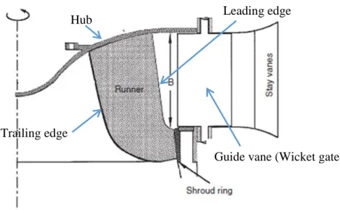
A Francis turbine comprises five main components: the spiral casing, stay vanes, guide vanes (wicket gates), runner and draft tube. Figure 1-3 shows a side view of a typical Francis turbine including the electric generator. Inside the spiral case; the axial flow is changed to radial flow. Then the guide vanes adjust the velocity and angle of the flow that reaches the runner in order to

(25)

control the power output (see Figure 1-4). The passing water rotates the runner about its axis. The rotational motion is converted to electric power through the runner shaft which is coupled with the generator. Finally, water flow passes in the draft tube to reach the lower reservoir. In this way, the draft tube acts as a diffuser to convert the residual energy of the flow into static pressure.

Figure 1-2: Operation areas of hydro turbines(Wagner et al., 2011)

(26)

1.3 Present work

1.3.1 Problematic

Recently, the hydroelectric power plants have been deemed to play a new role as a flexible supplier of energy in the modern electrical grid because of the non-dispatchable production by renewables, such as wind and solar power (Dörfler et al., 2013). Under such circumstances, the hydroelectric power plants have to operate under off-design conditions, while they have traditionally been designed for a stable demand and continuously running conditions.

In addition, the new exploitation strategies often lead to more frequent transient processes due to sudden variations of the operating conditions such as machine shut-down or start-up and power variations. These transient processes may have a detrimental impact on the electrical grid (Dörfler et al., 2013; Nicolet, 2007). Irregular transient processes such as load rejection, no-load conditions and runaway (see below) may also occur. In hydroelectric power plants, the transient processes produce complex and time-dependent flow phenomena which induce pressure fluctuations and unsteady stresses on the structure. These conditions may influence the mechanical safety of hydraulic machines. In general, off-design operating conditions have a damaging effect on hydroelectric power plants such as shortening the runner’s life, increasing cost of plant operation and losing power generation (Trivedi, 2014).

Figure 1-4: Side view of a typical Francis turbine layout (Round, 2004) Leading edge

Trailing edge Hub

(27)

Several studies have focused on improving the turbomachinery designs so as to efficiently decrease the influence of off-design conditions and transient processes. Nevertheless, these investigations must be evaluated and compared to provide the hydroelectric power industry with efficient and robust methodologies for complex unsteady operating conditions.

1.3.2 Transient processes

Some harmful transient processes which may occur in hydroelectric power plants are presented in this section.

1.3.2.1 Speed no-load

Speed no-load condition typically happens when turbines are in standby mode for immediate connection to the grid. In this regard, the turbine operates at synchronous speed without electricity production. The speed no-load condition may happen over a long period (B. Nennemann et al., 2014).

1.3.2.2 No-load and Runaway

No-load condition is one of the most harmful transient processes. This process happens if the control system of the hydroelectric power plant fails to close the guide vanes when the generator is disconnected from the grid, and this failure leads to an instant rise of the runner’s speed. The maximum speed attained by a runner is called runaway at full-gate opening and no-load speed at other guide vane angles. The value of runaway speed changes based on the turbine design, operation, and its setting. It may reach 150 to 350 % of its normal speed (Warnick, 1984).

1.3.2.3 Load Rejection

Load rejection occurs when the generator is disconnected from the network because grid parameters change beyond the generators prescribed range (Trivedi, 2014). In contrast to the runaway, during load rejection, the governor system of the turbine rapidly takes action to prevent the rotational speed from reaching an excessive value by closing the guide vanes. However, the rapid closing of the guide vanes may lead to pressure waves, which move forward and backward through the whole water passage. Consequently, it may lead to serious damage to hydroelectric power plants if not adequately managed.

(28)

1.3.3 Objectives

The main objective of this thesis is to develop and validate a methodology to predict the operation of a Francis turbine during load rejection based on the CFD simulations.

The main objective involves three specific objectives:

1. Developing a method based on the steady simulation for computing the runaway and no-load speeds(steady method)

2. Developing an approach for studying Francis turbine operation at runaway and no-load conditions using an unsteady simulation(unsteady method)

3. Developing the unsteady method for studying Francis turbine performance during load rejection by considering the movement of guide vanes.

The first objective of this thesis is to develop and validate a simple and fast method to calculate the runaway and no-load speeds using steady-state CFD simulations (steady method) based on the following essential phases:

 Development of an iterative algorithm that relies on a relation between turbine torque and speed coefficient

 Assessment of the steady method by computing no-load speed curves for the different Francis turbine cases

 Validation of the engineering quantities of the turbine computed by the steady method. The second objective is to develop and validate an approach using an unsteady simulation (unsteady method) for studying Francis turbines at runaway and no-load conditions with fixed guide vanes according to the following steps:

 Development of an algorithm using an unsteady CFD simulation coupled with a user function which computes the runner acceleration based on the angular momentum equation

 Development of the unsteady CFD simulation by computing the dynamic time step, and the friction torque on the hub and shroud in addition to the turbine runner torque

(29)

 Systematic comparison between steady and unsteady simulations for computing the runaway and the no-load speeds of the Francis turbine

 Comprehensive analysis of the evolution of the engineering quantities, unsteady pressure and flow physics inside the turbine at runaway and no-load conditions computed by unsteady method

 Comparison between unsteady simulations of Francis turbines for two geometry configurations: a complete turbine and a single runner/distributor passage in order to determine the influence of interface models: transient rotor-stator (TRS) and stage on the accuracy and computational cost.

The third specific objective is to evolve the unsteady method that simulates the Francis turbine during load rejection based on the following steps:

 Development of an algorithm for modeling the guide vane movement using the mesh deformation and re-meshing techniques.

 Assessment of the proposed methodology by computing the unsteady pressure, flow physics and turbine engineering quantities during a load rejection process

 Validation of unsteady loads and runner speed computed by the load rejection simulations.

1.3.4 Structure of the Document

This thesis is organized in the following manner. In Chapter 2, previous studies regarding the investigation of hydroelectric turbines during transient processes are described. Indeed, Chapter 2 presents the methods applicable to analyze operation of hydroelectric turbines during load rejection, runaway and at no-load conditions. The scientific approach for the present research as well as the publication strategy is presented in Chapter 3. The three articles resulting from this project are included as Chapters 4 to 6. The connection between the articles is discussed in Chapter 7. Finally, the conclusion summarizes the main contributions of the thesis, and provides recommendation for future studies.

(30)

CHAPTER 2 LITERATURE REVIEW

In recent years, several attempts have been undertaken to study hydroelectric turbines in off-design conditions and during transient processes. The main objective of this chapter is to provide a comprehensive review of the state-of-the art in this field. In this regard, the limitation and strength of the proposed methods such as the hydro acoustic, experimental and computational fluid dynamic methods are explained. This survey is limited to reaction hydroelectric turbines especially Francis, Kaplan, Bulb, and reversible pump-turbines.

2.1 One dimensional-hydro acoustic methods

The hydro acoustic theory uses a mathematical model based on the one-dimensional hyperbolic equations of the elastic water hammer propagation in a pipeline to represent the dynamic behavior of hydropower plants (Nicolet, 2007):

𝜕ℎ 𝜕𝑥+ 1 𝑔𝐴 𝜕𝑄 𝜕𝑡 + 𝜆𝑄|𝑄| 2𝑔𝐷𝐴2 = 0 (2-1) 𝜕ℎ 𝜕𝑡 + 𝑎2 𝑔𝐴 𝜕𝑄 𝜕𝑥 = 0 (2-2) with: 𝐴 : pipe cross-section [m2 ]; 𝑎 : wave speed [m/s]. 𝐷 : pipe diameter [m]; 𝑔 : gravitational acceleration [m/s2 ]; 𝑄: discharge [m3 /s]; ℎ : piezometric head [m]; λ : friction coefficient.

The set of equations can be solved by various methods such as the method of characteristics, the transfer matrix method and the impedance method. The next sections describe two important

(31)

methods: the method of characteristics and the impedance method for simulating hydroturbines during transient processes.

2.1.1 Method of characteristics

In the method of characteristics, equations (2-1) and (2-2), which are related to the elastic water hammer propagation in a pipeline, are solved using a mathematical technique which is called the method of characteristics. This technique changes the governing partial differential equations to ordinary differential equations (Joukowsky, 1900; Streeter et al., 1993; Swaffield, 1993).

The method of characteristics, because of its simplicity and high performance, is commonly used for solving the water hammer equations during transient events such as a sudden valve closure or opening in a pipe and duct system, starting or stopping pumps, and so on. However, the method of characteristics cannot be applied for predicting 3D unsteady flows in hydraulic turbines, since it is a one-dimensional approach based on the inviscid hypothesis.

Afshar (Afshar et al., 2010) used the implicit method of characteristics (IMOC) to simulate transient flow in the penstock due to the power plant load rejection. In this manner, the variation of head and flow rate parameters were accurately predicted.

During transient operations in hydropower plants, dropping local pressure under the vapor pressure induces a water column separation phenomenon which could damage the turbine runner and non-rotating parts. Pejovic (Stanislav Pejovic, 2004) studied water column separation during load rejection in an underground hydroelectric power plant with long tailrace. Pressure measurements at the draft tube cone and 1-D transient numerical modeling based on the water hammer theory were used to analyze water column separation. The results displayed a huge pressure rise after a drop due to the collapse of the large void which was formed because of the pressure reducing below the vapor pressure in the draft tube. Therefore, it was suggested to consider a minimum submergence of the turbine installation as a function of the rotational speed in order to control the excessive pressure drop and subsequent pressure rise due to large void collapse.

(32)

2.1.2 Impedance method

The impedance method may be used for solving the hyperbolic system of equations for compressible mass flow and momentum conservation which describe the dynamic flow behavior in a hydroelectric power plant. In the method of impedance, the fluid fluctuation is analyzed using vibration and electrical transmission line theories (Streeter et al., 1993).

Nicolet (Nicolet, 2007) modeled the hydraulic components based on the impedance method in the SIMSEN software for modeling electrical power networks systems in transient or steady state mode, in order to simulate transient phenomena in Francis turbines. In this regard, three models: hydraulic, electric and hydroelectric were used for studying the transient behavior of a power plant with two Francis turbines. The simulation was performed for hydroelectric power plant transient conditions such as load rejection. During the simulation, parameters such as rotational speed, pressure, and discharge were analyzed. Finally, the simulation using the hydroelectric model was found more beneficial because it considers the strong interactions between the electric and hydraulic parts. In addition, results obtained from simulations were applied to test new control strategies.

2.1.3 Limitation of hydro acoustic methods

Generally, hydro acoustic methods are appropriate for predicting water hammer, which dominates in the dynamic behavior of the entire hydraulic circuit during transient processes. These methods offer compromise in terms of computational effort and accuracy. Nevertheless, hydro acoustic methods depend on experimental data such as the turbine hill-chart in order to define the hydraulic resistance and inductance needed in transient simulations. Furthermore, hydro acoustic methods are not capable of predicting unsteady 3D flow features such as vortices, cavitation, and recirculation inside a hydro turbine.

2.2 Experimental methods

In recent years, experimental methods have been applied for analyzing the performance of hydraulic turbines during transient processes and off-design conditions due to advancement of measuring instruments and techniques. For instance, the experimental data collected from different hydroelectric power plants was used to develop a theoretical model. The model showed

(33)

that increased start-stop cycles may reduce the predefined refurbishment time of power plants by up to 50 % (Sjelvgren, 1997). Experimental studies (Hasmatuchi et al., 2011) were performed in a reduced scale model of a pump-turbine in order to analyze the flow unsteadiness under runaway transient and low-flow conditions. These experiments revealed unsteady vortex formation and break down for the turbine brake mode. The vortex destruction led to asymmetric unsteady pressure pulsations and strong vibration. Furthermore, experiments showed that swirling flow developed at the runner inlet during closure of the guide vanes. This swirling flow caused more flow separation, instability in the runner blade passage, and asymmetric loading on the blades (Antonsen, 2007).

Transient pressure measurements were performed (Trivedi et al., 2015; Trivedi et al., 2014; Trivedi, Cervantes, et al., 2013; Trivedi, Gandhi, et al., 2013) in a high head model Francis turbine during start-up, shut-down, load variations, load rejections, and spin-no-load covering the entire range of the turbine operation. The pressure fluctuations, measured on model tests, were normalized with either the net head (H) or the specific hydraulic energy (E) in order to transfer from the model turbine to the prototype (Trivedi, 2014). Measurements from model tests showed that movement of guide vanes during load acceptance and rejection increase the pressure difference between the pressure and suction sides of the blade. The largest pressure variation occurred during the partial load rejection at the trailing edge of the blade (Trivedi et al., 2014). Pressure measurements during spin-no-load showed that the instantaneous amplitude of unsteady loads was similar to that computed for the critical transient conditions such as load variation, start-stop, emergency shutdown, and total load rejection (Trivedi et al., 2015). (Trivedi et al., 2014) indicated that the maximum amplitudes of the unsteady pressure fluctuations in a high head model Francis turbine at runaway condition were 2.1 and 2.6 times that of the pressure loading at the best efficiency operating point in the vaneless space and runner, respectively.

The pressure fluctuations on the runner blade of a propeller turbine were measured during a runaway test (Houde et al., 2012). The post-processing of experimental data showed that the main source of pressure fluctuations in the runner is associated with instabilities in the draft tube flow.

(34)

2.2.1 Limitation of experimental methods

Transient measurements are usually performed on sites or in labs with prototypes and model test turbines, respectively. Although, there has been an advancement of new measuring instruments and techniques, the collection and application of experimental data has been partial during transient processes because of difficulties. For instance, the startup or total load rejection of a prototype turbine may be damaging and expensive due to the fact that it induces strong unsteady loads on the turbine during the transient process. For instance, one turbine start-stop cycle might shorten the predefined refurbishment period by15 hours (Nilsson, 1997).

Moreover, model testing is widely used for studying the flow field in hydroelectric turbines. However, it is required to scale up the experimental data in order to use in designing and manufacturing the prototype. Generally, the basic parameters such as head, discharge, power, and speed can be transferred from a model test to prototype using similarity laws. Nevertheless, the transformation of pressure fluctuations may result in large scaling errors. For instance, a scaling error of 20-50% was reported over the extended turbine operating range (Alligné et al., 2010; Dorfler, 2009; Ida, 1989).

2.3 Computational fluid dynamics (CFD)

Over the past decade, increase in the computational capacity and advancements in numerical techniques have allowed to simulate hydraulic turbines during transient processes using CFD. Nevertheless, the numerical simulation of hydraulic turbines at off-design conditions and near no-load operation is challenging because the flow physics are complex and dominated by vortex formation in all parts of the turbine as well as backflow zones (Dörfler et al., 2013).

Table 2-1 summarizes the characteristics of the most relevant CFD simulations carried out for hydraulic turbines in different transient processes. The majority of these studies solve unsteady viscous flow in order to predict time-dependent phenomena. The steady-state simulations of a Francis turbine were performed to compute the pressure loading on the runner blades, hub and shroud hydraulic surfaces (Melot et al., 2014). Validation of simulation results with experimental measurements showed good agreement for strain calculations.

In addition, Table 2-1 shows that the time-averaged turbulence models such as the two equations 𝑘 − 𝜀 and 𝑘 − 𝜔 are generally used in these simulations. These models require substantially less

(35)

computational effort than sophisticated turbulence models such as the Reynolds stress model or filtering methods such as Large eddy simulation (LES).

The modelling of the variation in turbine speed is necessary during transient processes such as load rejection, start-stop and emergency shutdown. Most studies in Table 2-1 computed the runner acceleration or deceleration using angular momentum equations as follows, through a user function which is coupled with a CFD solver:

d T

dt I



  (2-3).

where T denotes the total torque on the main turbine axis acting on the runner, and I is the mass moment of inertia of rotating components. The torque may be computed from a CFD solver by hydraulic forces including pressure and shear forces acting on runner blades and hub surfaces. After a discretization, the runner angular speed is computed as follows:

1 n n T t I      (2-4).

where index n indicates the time step number in the unsteady simulation.

Experimental data was used to set the runner speed during some of the processes. For instance, (Fortin et al., 2014) updated the runner rotational speed based on the measurements during a runaway simulation of a model propeller turbine. These simulations showed that the numerical torque decreased more slowly than the actual torque in experiments. In addition, the amplitude of pressure fluctuations was underestimated in CFD simulations.

Furthermore, Table 2-1 indicates the computational domains used in each study, which generally consists of the complete distributor (stay vanes and guide vanes), complete runner and draft tube, despite the high computational effort. In addition, a transient rotor-stator interface model (TRS) was frequently used for matching stationary and rotating parts.

(Nicolle et al., 2012) evaluated various numerical setups for modeling a low head Francis turbine during a startup process, as shown in Table 2-1. A transient rotor-stator interface model was applied in all simulations. The unsteady simulations showed that a configuration including one runner and distributor channel may predict the main turbine physics such as runner speed

(36)

variation during runner acceleration. In addition, considering the draft tube in simulations improved the results by allowing for better pressure recovery. Finally, the simulation with complete turbine allowed for capturing rotating stall in the vaneless space at the speed no-load regime.

The flow behavior in a Francis turbine during load rejection was investigated using the hypothesis of “frozen” hydraulic conditions (Côté et al., 2014). The unsteady RANS equations were solved on the fixed boundary conditions related to a specific operating condition on the runaway hill chart. The frozen rotor stator ("ANSYS CFX-User manual,") was used for matching rotating and stationary parts so that they each have a fixed relative position during the calculation. The analysis of flow revealed a downward tangential flow near the band and draft tube cone wall, and strong pumping flow near the draft tube cone center. Interaction of the inlet and reversed flow in the runner resulted in very unsteady flow patterns which induced dynamic loads.

In load rejection simulations, the modelling of the movement of guide vanes is a challenging task. Generally, after each blade movements, the internal hydrodynamic mesh must be adjusted to the newly computed boundary nodes. Large displacement during transient processes degrade the mesh quality significantly (Casartelli et al., 2014). Therefore, developing a robust and efficient mesh deformation technique is necessary.

In order to simulate the opening of guide vanes, a user defined function was applied (Nicolle et al., 2012), which updated the mesh around the guide vane at each time step based on a prescribed motion. (J. T. Liu et al., 2012) simulated guide vane shutoff of a prototype pump-turbine during a load-rejection process using a dynamic mesh method. However, the dynamic mesh method details were not explained in this paper. The simulations predicted that a vortex rope appears inside the draft tube before reaching the turbine zero-torque condition.

(Casartelli et al., 2014) investigated unstable characteristics which caused oscillations in the reversible pump-turbines at no-load and in the turbine brake operation. The unsteady RANS equations were solved using the OPEN FOAM toolbox. The movement of the guide vanes was simulated by an explicit mesh deformation technique, based on Inverse Distance Weighting (IDW) interpolation of the boundary node movement to the interior of the flow domain. The proposed mesh motion method was time-efficient and memory-efficient (Witteveen et al., 2009).

(37)

The simulations predicted a complex flow inside the computational domain, including strong tangential flow at the guide vane outlet, and reversed flow at the hub and shroud of the runner. (Y. Li et al., 2015) applied an active dynamic mesh technique in order to simulate the opening and closing of guide vanes in a Bulb hydraulic turbine in start transition process and load rejection. The technique was based on the simple concept of regenerating the mesh for each time step during large displacements. However, the method introduced inevitable interpolation errors during the simulation that caused an increase of the computational cost. The load rejection simulation depicted reflux in the runner entrance, a vortex phenomenon at the guide vanes and the draft tube, which caused significant swing and vibration of the Bulb turbine.

The emergency shutdown process of a ring gate was investigated numerically in a low head Francis turbine (Xiao et al., 2012). The unsteady RANS equations with the 𝑘 − 𝜀 RNG turbulence models were solved on the full flow passage of the Francis hydraulic turbine. Dynamic meshes and sliding meshes were used to simulate the movement of the ring gate. Moreover, the numerical analysis included the study of air and liquid multiphase flows in the flow passage using a mixture model. The analysis of results showed that the ring gate experiences a certain overturning torque due to a difference in pressure distribution between inner and outer surfaces. The turbine group vibration and uniform flow field in the guide vanes are observed at the end of closing.

Table 2-1 shows that many studies focused on the analysis of reversible pump-turbines for conditions around the no-load condition (Casartelli et al., 2014; Widmer et al., 2011). In these studies, the main goal was to investigate and predict the characteristic instability in the S-shaped region of the characteristic curve and as well the radial force imbalance on the machine caused by rotating stall.

In addition, Table 2-1 shows that the runaway transient in Francis turbines was studied by (Cherny et al., 2010; Jinwei LI et al., 2009; J Li et al., 2010). These investigations depicted the reversed flow in the runner and the vortex rope in the draft tube, which induces pressure fluctuations. The evolution of engineering quantities computed (Jinwei Li et al., 2007) showed that the runner speed increased by 58% and flow rate decreased by 14% at runaway.

(38)

2.3.1 Limitation of Computational fluid dynamics

As mentioned in the previous section, CFD simulations of hydraulic turbines during transient processes and off-design conditions are very challenging due to complex flow structures consisting of irregular backflows and vortices. Simulations must be time-dependent with high grid resolution in order to provide realistic flow prediction. Therefore, the CFD simulations depend on high computational effort (Dörfler et al., 2013). In addition, (Magnan et al., 2014) indicated challenges for assessing the grid sensitivity of hydroelectric turbine CFD simulations. Grid independence analysis for complex, detached flows involved many challenges among which: making refined meshes and comparing with experiments.

Besides, the complex flow structures lead to large stochastic pulsations of the flow, pressure, and guide vane torque. Thus, the assessment of unsteady flow is difficult due to wide-band fluctuations in CFD simulations of transient processes (Dörfler, Sick et al., 2013). For instance, (B Nennemann et al., 2014) showed that turbulence model and numerical dissipation have a significant influence for predicting dynamic loads on the runner at no-load conditions.

In addition, the validation of unsteady CFD simulations of the flow close to no-load condition is partial because the measurements of unsteady pressure distribution in the runner and draft tube are very hard and expensive to obtain (Dörfler et al., 2013).

(39)

Table 2-1 Literature review of CFD simulations of hydraulic turbines during transient processes Author Turbine type Transient process Computational domain Mesh (Mil) Code Analysis type Interface model Turbulence model Runner speed variation (Kolšek et al., 2006) Bulb

turbine _Shutdown Full distributor, runner, _{draft tube} _-- _ICCM _Unsteady _--

Standard 𝑘 − 𝜀 momentum Angular (Jinwei Li et al., 2007) Francis Turbine Runaway

Full spiral casing , distributor, runner, draft

tube -- -- Unsteady TRS RNG 𝑘 − 𝜀 momentum Angular (Li, Yu et al., 2010) Francis Turbine Load rejection

Penstock, full spiral casing , distributor,

runner, draft tube 3.4 Fluent Unsteady TRS

RNG

𝑘 − 𝜀 momentum Angular

Model Francis turbine

Runaway Full spiral casing , distributor, runner, draft

tube 2.4 Fluent Unsteady TRS RNG k − ε

Angular momentum (Cherny et al., 2010) Francis Runaway

One distributor channel, runner channel and draft

tube 0.45 -- Unsteady Periodic-stage Standard 𝑘 − 𝜀 momentum Angular (S. Liu et al., 2010) Model Kaplan turbine

Runaway Casing, distributor, and _{runner passages and}

draft tube 1.777 Fluent Unsteady

Sliding mesh RNG 𝑘 − 𝜀 momentum Angular (Widmer et al., 2011) Prototype pump-turbine Brake operation

tube 5 CFX Unsteady TRS

Standard

(40)

Table 2-1: Literature review of CFD simulations of hydraulic turbines during transient processes “cont’d”

Author

Turbine type

Transient

process Computational domain

Mesh (Mil) Code Analysis type Interface model Turbulenc e model Runner speed variation (J. T. Liu et al., 2012) Prototype pump-turbine Load rejection

tube 5 CFX Unsteady TRS RANS v2-f Angular momentum (Yan et al., 2012) Model pump-turbine Runaway

tube 7.7 CFX Unsteady TRS Standard k − ε Constant (Huang et al., 2012) Francis Load-rejection

Casing, distributor, and runner passages and draft

tube 2.19 Fluent Unsteady Sliding

RNG k − ε momentum Angular (Nicolle et al., 2012) Francis Startup

One channel distributor, runner, DRA, DRA360,

DRAS 360 0.36 CFX Unsteady TRS

Standard

k − ε momentum Angular One channel distributor,

runner, draft tube 0.63 CFX Unsteady TRS

Standard

k − ε momentum Angular 360 distributor , runner,

draft tube 6.49 CFX Unsteady TRS

Standard

k − ε momentum Angular 360 spiral casing,

distributor, runner, draft

tube 14.4 CFX Unsteady TRS

Standard

(41)

Table 2-1: Literature review of CFD simulations of hydraulic turbines during transient processes “cont’d” Author Turbine type Transient process Computational domain Mesh (Mil) Code Analysis type Interface model Turbulence model Runner speed variation (Casartelli et al., 2014) Pump-turbine Speed-no load

Full spiral casing , distributor, runner,

draft tube --

Open

FOAM Unsteady TRS 𝑘 − 𝜔 SST Constant (B. Nennemann et al., 2014) Francis No-load condition 1st setup: full distributor, runner, draft tube 5 CFX Unsteady TRS 𝑘 − 𝜀 & SAS Constant (Melot et al., 2014) Francis Speed-no-load Casing, distributor, and runner passages and draft

tube -- CFX steady stage

Standard 𝑘 − 𝜀 -- (Côté et al., 2014) Francis Load-rejection 1/24 distributor and full runner, draft

tube -- CFX Unsteady Frozen- rotor-stator -- -- (Fortin et al., 2014) Model propeller turbine Runaway Full semi-spiral casing, distributor

,runner draft tube 7 CFX Unsteady TRS

Standard

(42)

2.4 Summary

Transient simulation of runaway, no-load conditions and load rejection events in hydraulic turbines is a very active field of the research, where great efforts are still required to provide design engineers with efficient and robust simulation methodologies. There are several competing approaches under development that must be evaluated and compared. Based on the previous literature review, it appears that thorough validation of steady and unsteady CFD simulation approaches for runaway, no load condition and load rejection evens is still required. This constitutes the research topic covered in the present thesis.