UNIVERSITÉ DE MONTRÉAL
A GEOMETRIC APPROACH TO CONVERTING CAD MODELS TO CAM
MODELS: AN APPLICATION ON AERONAUTICAL STRUCTURE PARTS
HUA LU
DÉPARTEMENT DE GÉNIE MÉCANIQUE ÉCOLE POLYTECHNIQUE DE MONTRÉAL
THÈSE PRÉSENTÉE EN VUE DE L’OBTENTION DU DIPLÔME DE PHILOSOPHIAE DOCTOR
(GÉNIE MÉCANIQUE) NOVEMBRE 2012
UNIVERSITÉ DE MONTRÉAL
ÉCOLE POLYTECHNIQUE DE MONTRÉAL
Cette thèse intitulée
:A GEOMETRIC APPROACH TO CONVERTING CAD MODELS TO CAM
MODELS: AN APPLICATION ON AERONAUTICAL STRUCTURE PARTS
présentée par: LU Hua
en vue de l’obtention du diplôme de : Philosophiae Doctor a été dûment acceptée par le jury d’examen constitué de:
M. VADEAN Aurelian, Doct., président
M. MASCLE Christian, Doctorat ès Sciences, membre et directeur de recherche M. MARANZANA Roland, Doct., membre et codirecteur de recherche
M. BALAZINSKI Marek, Ph.D., membre M. LAPERRIÈRE Luc, Ph.D., membre
DEDICATION
iv
ACKNOWLEDGEMENT
The author is greatly appreciative to his supervisors Professor C. Mascle and Professor R. Maranzana, for their encouragement, invaluable discussion and enlightening guidance. I deeply appreciate their efforts for providing me the unique opportunity to pursue my PhD study and bringing me into the CAD/CAM domain. Their wide knowledge and deep insights into scientific problems, sincere attitude and enthusiasm for the research will continue to encourage the author.
Special thanks are given to Dr. O. Msaaf for his constructive discussions and guidance at the beginning of the research. Particular thanks are given to Ms. S. Chalut, Mr. J. Ruby, and Ms. R. Li for their help and encouragement.
Finally, the author would like to express his warmest gratitude to his wife and son for their long-term consistent support and encouragement.
RÉSUMÉ
La conversion d'un modèle de CAO en un modèle de FAO est la première étape de fabrication intégrée par ordinateur. Les principaux problèmes qui concernent la conversion sont les suivants: définir des volumes de matériau amovible géométriquement, vérifier les accessibilités aux volumes ainsi obtenus, associer les opérations d'usinage avec ces volumes individuellement, sélectionner les outils de coupe, mettre en séquençage les opérations d'usinage et assigner une machine pour exécuter le processus.
La détermination des volumes individuels de matériel amovible est le premier problème de la conversion. Dans les dernières décennies, de nombreuses approches ont été développées avec d'énormes efforts, mais aucune étude à ce jour a examiné de manière exhaustive les approches pour générer des volumes de matériau amovible pour traiter des pièces complexes, telles que celles qu’on rencontre dans en aéronautique dans la partie structurelle. Dans la perspective de définir les volumes du matériau amovible, les méthodes existantes se limitent aux fonctions prismatiques. L'objectif principal de cette recherche était de développer des approches systématiques, pour générer automatiquement l'ensemble des volumes de matières amovibles selon les modèles 3D d’une pièce aéronautique structurelle. Il faut alors partir du brut (un morceau de matière première) et usiner toutes les surfaces requises. Grâce à l'outil mathématique disponible des opérations booléennes, il est possible de séparer des géométries volumiques très complexes en volumes plus petits relativement simples. La décomposition du volume delta présente des avantages dans la création des volumes amovibles. Dans cette recherche, les approches de décomposition de volume ont été développées dans le but que chaque volume de matériau puisse être usiné en une seule opération d'usinage. Des arêtes concaves impliquent éventuellement des opérations d'usinage différentes. La détection du bord concave est la première étape de la décomposition de volume intérieur. Dans cette étude, une approche mathématique a été développée afin de vérifier la concavité d'une arête dans la limite d'un modèle solide 3D et une approche de détection des bords concaves est proposée.
Générer des faces de séparation est une étape clé pour définir un volume décomposé. Selon la complexité de l'élément de construction, les algorithmes sont conçus pour créer différents types de décompositions de faces correspondant à des formes locales de la pièce à décomposer. L’union des faces est un outil puissant pour des volumes distincts délimités par des faces de
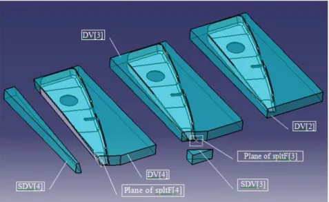
vi géométries complexes. Cette recherche propose des procédures récursives de décomposition. En utilisant les approches proposées par le modèle de conception 3D, un composant aéronautique de structure est converti en volumes de matériau amovible, nommé sous delta volume (SDV), au moyen de la décomposition du volume delta.
Des approches dédiées à l'identification et la décomposition d’une îlot qui constitue une catégorie spéciale de SDV ont été développées. Nous avons traités les problèmes entourant le cas du trou incliné en détail. Les sujets abordés comprennent la création d'une face d'accès plan, l'expansion du brut, la redéfinition des volumes liés aux SDV et la combinaison de SDV adjacents au trou SDV, etc.
Le deuxième problème de la conversion est de définir les opérations d'usinage correspondant à des volumes individuels. Il est différent de créer des motifs et des zones de cartographie détectés dans une partie de la pièce avec les modèles proposés par d'autres recherches dans les études précédentes. Cette recherche aborde l'attribution des opérations d'ébauche à des SDV qui ont été élaborés en accord avec les propriétés et les positions relatives de la partie face de délimitation spécifique SDV respective. L’affectation d'opérations d'ébauche à des SDV individuels présente des avantages par rapport à une ébauche de toute la partie avec un seul outil. Pour les instances, tout d'abord, pour atteindre une plus grande efficacité de coupe des SDV différents peuvent nécessiter des outils de diamètres différents, d'autre part, très souvent, dans la pratique, il n'est pas nécessaire de balayer un outil dans tout le volume d'un SDV extérieur (un SDV entourant la partie), parce que la séparation du SDV de la pièce peut être réalisée en faisant passer un outil de balayage ou une partie de la surface de délimitation du SDV.
Le troisième problème est de déterminer les caractéristiques d'usinage des SDV individuels. Chaque SDV a ses attributs d'usinage spécifiques, comme la face d'accès, le point d'accès et la direction d'accès, le type et les paramètres de l'outil. Dans cette recherche ces attributs sont déterminés selon les géométries des SDV individuels. Les approches pour déterminer la direction d'accès ont été développées avec l’intention que venant ainsi déterminer l’accès toutes les visages puissent être accessibles, si c'est possible. L'usinabilité d'une partie a été vérifiée pour deux aspects : l’accessibilité angulaire et l’accessibilité linéaire des SDV individuels. Pour vérifier l'accessibilité angulaire, les approches proposées déterminent la posture de l’outil plat et celle de l’espace-outil (notée TPF/TPS). Un TPF/TPS non vide garantit l'accessibilité angulaire d'une
face. Et une intersection non vide de la TPF/TPS de toutes les faces de la part d'un SDV implique qu’il est accessible selon une seule direction. L’accessibilité linéaire a été vérifiée conformément aux orientations spécifiques.
La quatrième question de la conversion dans cette recherche est le séquençage des opérations. Des approches sont proposées pour générer une séquence de mise en service du brut selon les attributs d'usinage et les positions relatives des volumes décomposés. D’autres approches ont été élaborées en vue de renouveler les paramètres de l'outil comme certaines modifications devraient être apportées à la séquence.
viii
ABSTRACT
Conversion of a CAD model to a CAM model is the initial step of computer integrated manufacturing. Main issues concerning the conversion are as follows: defining volumes of removable material geometrically, verifying accessibilities to so obtained volumes, associating machining operations with these volumes individually, selecting cutting tools, sequencing machining operations, and assign a machine to perform the process.
Determination of individual volumes of removable material is the first issue of the conversion. In the past decades many approaches have been developed by enormous efforts but no study up to date has comprehensively discussed approaches to generate volumes of removable material for producing a complex aeronautical structural part. In the perspective of volumetric definition of removable material, existing methods are limited to prismatic features. The main objective of this research was to develop systematic approaches to generating automatically the complete set of volumes of removable material according to the 3D models of both an aeronautical structural part to be produced and the stock (a piece of raw material) to be machined. Due to powerful mathematical tool of Boolean operations available for separating very complex volumetric geometries into relatively simple smaller volumes, delta volume decomposition has advantages in generating removable volumes. In this research volume decomposition approaches were developed for the purpose that every volume of material can be machined in one machining operation. Concave edges imply possible requirement of different machining operations. Detecting concave edge is the premier step of interior volume decomposition. In this study a mathematical approach was developed to verify the concavity of an edge in the boundary of a 3D solid model. Approaches to detecting concave edges were proposed.
Generating splitting faces is the key step to define a decomposed volume. According to the complexity of the structural component, algorithms are developed to create different kinds of splitting faces corresponding to local shapes of the part to perform decompositions. Face union is a powerful tool to separate volumes bounded by faces of complex geometries. This research proposed recursive procedures of decomposition. Using the proposed approaches the 3D design model of an aeronautic structural component is converted into volumes of removable material (named sub delta volume and denoted SDV in this research) by means of delta volume decomposition.
Approaches dedicated to identifying and decomposing an island which is a special category of SDVs are developed. Issues about an inclined hole are discussed in detail. Topics discussed include creation of a planar access face, expansion of the stock, redefinition of related sub delta volumes, and combination of SDVs adjacent to the hole SDV etc..
The second issue of the conversion is to define machining operations corresponding to individual volumes respectively. Different from creating patterns and mapping areas detected in a the part with the patterns as proposed by other researches in previous studies, in this research approaches to assigning roughing operations to SDVs were developed in accordance with the properties and the related positions of part faces bounding specific SDVs respectively. Assigning roughing operations to individual SDVs respectively has advantages over that to roughing the whole part with one tool. For instances, first, to achieve higher cutting efficiency different SDVs may require tools of different diameters, second, very often in practice it is not necessary to sweep a tool all over the volume of an exterior SDV (a SDV surrounding the part) because separating the SDV from the workpiece can be conducted by passing a tool sweeping one or some of the boundary face(s) of the SDV.
The third issue is to determine the machining attributes of individual SDVs. Every SDV has its specific machining attributes, such as access face, access point, and access direction, tool type and parameters. In this research these attributes are determined according to the geometries of individual SDVs respectively. Approaches to determining the access direction were developed under such an intention that from the so determined access direction all part faces are accessible, if it is possible. Machinability of a part was verified from two aspects: angular and linear accessibility of individual SDVs. For verifying angular accessibility, the proposed approaches determine the tool posture flat and tool posture space (denoted TPF/TPS). A non-empty TPF/TPS guarantees angular accessibility of a face. And a non-empty intersection of the TPF/TPS of all part faces of a SDV implies being accessible from one direction. Linear accessibility was verified in accordance to specific direction(s).
The fourth issue of the conversion discussed in this research was operation sequencing. Approaches are proposed to generate an initial operation sequence for roughing according to the machining attributes and relative positions of the decomposed volumes. Approaches were developed to renew tool parameters as some modifications should be made to the sequence.
x
TABLE OF CONTENTS
DEDICATION ... III ACKNOWLEDGEMENT ... IV RÉSUMÉ ... V ABSTRACT ... VIII TABLE OF CONTENTS ... X LIST OF TABLES ... XV LIST OF FIGURES ... XVI LIST OF SYMBOLS AND ABBREVIATIONS... XX LIST OF ANNEXES ... XXIIIINTRODUCTION ... 1
CHAPTER 1 STATE OF THE ART ... 6
1.1 Feature Recognition ... 7
1.1.1 Concept of Feature ... 7
1.1.2 Feature Recognition Approaches ... 9
1.1.3 Efforts in feature classification and standardization ... 18
1.1.4 Limitations ... 18
1.2 CAPP ... 19
1.2.1 Operation Sequencing ... 19
1.2.2 Tool and Machine Selection ... 21
1.3 CAD/CAM Integration ... 22
1.4 Synthesis and objectives ... 23
1.4.1 Limitations of existing systems and research ... 24
1.4.3 Research Objectives ... 28
CHAPTER 2 CONCEPTION AND METHODOLOGY ... 29
2.1 Assumptions ... 29
2.2 Methodology ... 30
2.2.1 Geometry decomposition ... 31
2.2.2 Manufacturing attribute determination ... 32
2.2.3 Machining operation selection ... 33
2.2.4 Operation sequencing ... 33
2.3 Terminology ... 34
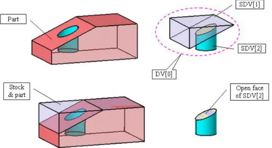
2.3.1 Original delta volume and current delta volume ... 34
2.3.2 Sub delta volume ... 35
2.3.3 Delta volume decomposition ... 36
2.3.4 Open face and closed face ... 38
2.3.5 Adjacency with other SDV ... 38
2.3.6 Top/bottom and wall face ... 38
2.3.7 Milling operation attributes ... 39
2.3.8 Access face ... 39
2.3.9 Access point ... 39
2.3.10 Access direction /Tool Approach Direction ... 40
2.3.11 Operation Sequencing ... 41
2.4 The Contributions ... 42
CHAPTER 3 DELTA VOLUME DECOMPOSITION ... 43
3.1 Determination of DV[0] ... 43
xii
3.2.1 One SDV by one splitting ... 45
3.2.2 Location of a splitting face ... 45
3.2.3 From outside towards inside ... 46
3.2.4 Creating a simple face ... 46
3.2.5 Splitting faces ... 47
3.3 Procedures and Algorithms ... 47
3.3.1 Summary of decomposition approaches ... 48
3.3.2 Data structure ... 50
3.3.3 Denotation of Initial data ... 51
3.3.4 Coordinate systems ... 53
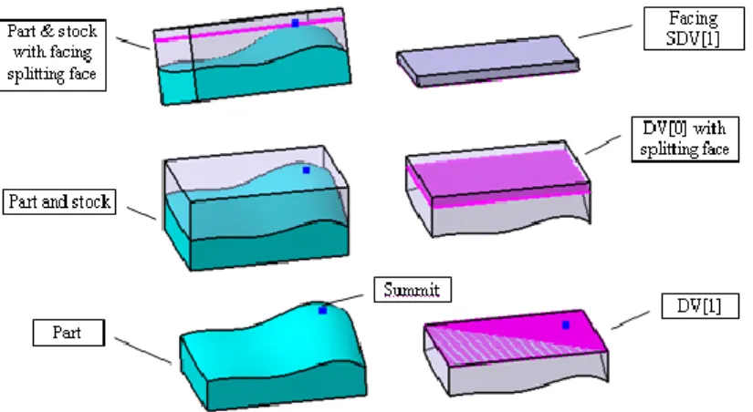
3.3.5 Facing volume SDV[1] determination ... 54
3.3.6 Determination of exterior SDVs ... 61
3.3.7 Basic Concepts for identifying interior SDV ... 71
3.3.8 Island SDV ... 75
3.3.9 Interior DV decomposition ... 79
3.4 An example of multi-pocket ... 90
CHAPTER 4 DETERMINATION OF MILLING ATTRIBUTES ... 97
4.1 Machining attributes ... 97
4.2 Determination of access position ... 98
4.2.1 Identification of open face and non-part edge ... 98
4.2.2 Access points of a general SDV ... 99
4.2.3 Access point of hole SDV ... 101
4.3 Redefinition of stock geometry ... 103
4.3.2 Geometry of final stock (SF) – single expansion vector ... 107
4.3.3 Geometry of final stock (SF) – multiple expansion vectors ... 110
4.4 SDVs Updating ... 114
4.4.1 Redefinition of inclined hole SDV ... 114
4.4.2 Final periphery SDV ... 115
4.4.3 Subdivision of SDVs intersected by FCC ... 118
4.5 Tool axis orientation ... 120
4.5.1 Parallel to Z axis ... 121
4.5.2 Perpendicular to access face or bottom face ... 121
4.5.3 Coincident with the axis of rotating volume ... 122
4.5.4 Tool axis for linear side SDV ... 123
4.5.5 Detecting folded face ... 126
4.5.6 Access direction to a folded side face ... 129
4.6 Angular operability ... 131
4.6.1 Capacity cone ... 131
4.6.2 Tool posturing plane ... 132
4.6.3 Tool posture flat/space (TPF/TPS) ... 134
4.6.4 Pivoting control point ... 136
4.6.5 Required pivot angle ... 139
4.7 Linear accessibility and collision ... 141
4.8 Assign machining operation to a SDV ... 142
4.9 Tool length, Diameter and Tip ... 144
4.9.1 Tool length ... 144
xiv
4.9.3 Type of tool tip ... 146
4.10 Operation sequence generation ... 147
CHAPTER 5 APPLICATION OF ATTRIBUTES ANALYSIS ... 150
5.1 Access face ... 151
5.2 Access point ... 153
5.3 Tool axis vectors ... 153
5.3.1 Tool axis vector of SDV[4] ... 154
5.3.2 Tool axis vectors of SDV[19] ... 155
5.4 Length of cutting edge ... 158
5.5 Diameter of tool ... 160
5.6 Type of tool tip and operation assigning ... 161
5.7 Operation sequencing ... 163
CONCLUSION AND RECOMMENDATIONS ... 166
REFERENCES ... 169
ANNEXES ... 176
LIST OF TABLES
xvi
LIST OF FIGURES
Figure 1-1 Feature Examples [11] ... 9
Figure 1-2 Feature conversion with graph grammar [35] ... 12
Figure 1-3 Hint-based slot recognition process [14, 39] ... 14
Figure 1-4 Convex Hull Decomposition [23] ... 15
Figure 1-5 Decomposition and recomposition procedures [11, 48] ... 16
Figure 1-6 Cell decomposition of the delta volume [11] ... 17
Figure 2-1 DV, SDV and open face ... 35
Figure 2-2 Multi TADs required removable volume ... 40
Figure 2-3 Axial accessibility and side accessibility ... 41
Figure 3-1 Sample part I and delta volume DV[0] ... 44
Figure 3-2 Difference between splitting by a face and a plane ... 45
Figure 3-3 A planar splitting face passing through the summit of a curved face ... 46
Figure 3-4 United splitting faces ... 47
Figure 3-5 Flow chart of delta volume decomposition ... 49
Figure 3-6 Reference systems of part, stock and DV ... 53
Figure 3-7 Top face of DV[0] ... 55
Figure 3-8 Extremum and splitting face ... 57
Figure 3-9 Determination of volumetric SDV[1] ... 58
Figure 3-10 Wall faces of SDV[1] ... 59
Figure 3-11 Flowing chart for exterior SDV determination ... 61
Figure 3-12 Planar face Ex and SDV[2] ... 62
Figure 3-13 Exterior SDVs split with planes ... 65
Figure 3-15 Splitting with face union UF ... 70
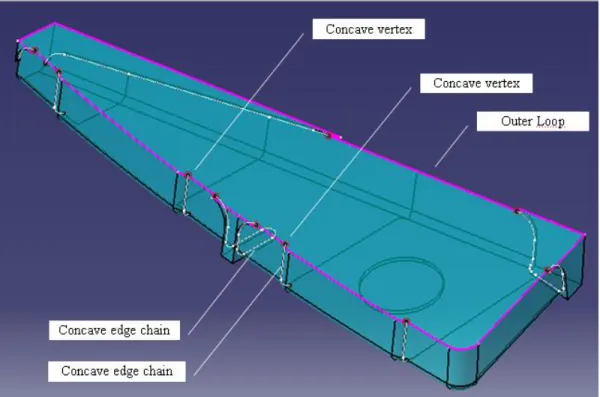
Figure 3-16 Example of concave vertices ... 71
Figure 3-17 Example of concave edge ... 72
Figure 3-18 Example of front/back concave vertices ... 74
Figure 3-19 An example of island SDV and DV update ... 78
Figure 3-20 An example of semi-island in a DV ... 79
Figure 3-21 Example of Echain[j] meets vertex Q of the inner loop of f ... 81
Figure 3-22 Concave vertices and concave edge chains ... 82
Figure 3-23 An example of Case 1 ... 84
Figure 3-24 An example of Case 1 ... 85
Figure 3-25 An example of Case 2 ... 86
Figure 3-26 An example of Case 3 ... 87
Figure 3-27 An example of Case 4 ... 89
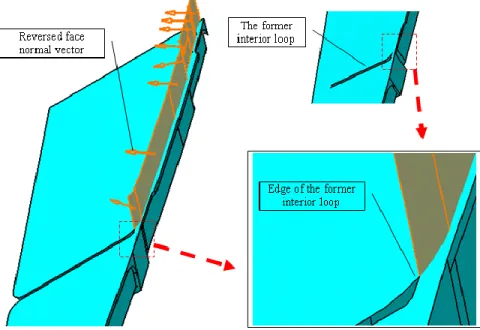
Figure 3-28 An example of reversing positive side of a UF ... 90
Figure 3-29 Decomposition of interior volume ... 90
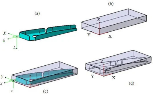
Figure 3-30 Part II - an aerospace structure part ... 91
Figure 3-31 Relative positions of part II and the stock ... 91
Figure 3-32 The initial delta volume DV[0] of sample part II ... 92
Figure 3-33 Extremum in positive z direction of sample part II ... 93
Figure 3-34 Separating SDV[1] from DV[0] ... 94
Figure 3-35 Decomposition of exterior and island SDVs of sample part II ... 95
Figure 3-36 Concave vertices in the outer loop of the top face of DV[18] ... 96
Figure 3-37 Completed decomposition of sample part II ... 96
xviii
Figure 4-2 Position vectors of specific points ... 104
Figure 4-3 Circle CC and extended hole SDV ... 106
Figure 4-4 Example of the extension of initial stock ... 110
Figure 4-5 Redefinition of the inclined hole SDV ... 115
Figure 4-6 Example of defining final periphery SDV ... 117
Figure 4-7 Subdivisions of SDVs ... 120
Figure 4-8 Tool axis orientation – perpendicular to the top/bottom face ... 122
Figure 4-9 Center line and Plane_Q ... 124
Figure 4-10 Example of folded face ... 127
Figure 4-11 Pivoting capacity cone ... 132
Figure 4-12 Tool posture flat/space ... 135
Figure 4-13 Tool postures for side edge cutting mode ... 137
Figure 4-14 Tool postures in tip cutting mond ... 138
Figure 5-1 Relative positions of example SDVs of Part II ... 150
Figure 5-2 Boundary faces f1, f2,…, f6 of SDV[4] ... 151
Figure 5-3 Intersections of SDV[4] and Part II ... 151
Figure 5-4 Boundary faces of SDV[19] (turned down for better view effect) ... 152
Figure 5-5 Access points of SDV[4] ... 153
Figure 5-6 Access points of SDV[19], SDV[21] and SDV[24] ... 154
Figure 5-7 Normal vectors of the open faces of SDV[4] ... 154
Figure 5-8 Projections of the boundary faces of SDV[4] ... 155
Figure 5-9 Tool axis vectors of SDV[21 and SDV[24] ... 155
Figure 5-10 Normal vectors and curve C of part faces of SDV[19] ... 156
Figure 5-12 Tool axis vector of SDV[19] ... 158
Figure 5-13 Minimum length of tool for machining SDV[19] ... 159
Figure 5-14 Multi view of SDV[21] ... 159
Figure 5-15 Minimum tool length for SDV[21] ... 160
Figure 5-16 Tool diameter for SDV[24] ... 160
Figure 5-17 Tool diameter for SDV[24] ... 161
Figure 5-18 Faces and normal vectors of SDV[24] ... 162
Figure 5-19 Facing SDV and interior SDVs of Part II ... 163
Figure 5-20 Procedures of putting the SDVs in the operation list ... 164
xx
LIST OF SYMBOLS AND ABBREVIATIONS
, ,
a b c The position vectors of extreme of CC in directions k ,1 k ,2 k 3
Brep Boundary representation
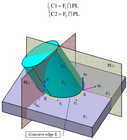
C1, C2 The intersections of PL with F1 and F2
CC Circle
CD Cell-based decomposition
CE[j] Concave edge
CV[j], CV[k] Concave vertex
CV Concave vertex
DV Delta volume
DV[0] The original delta volume
e Edge
E The expansion vector
e
i Set of edgesk
e Edge
Echain[j] Concave edge chain
k
ec The edge where point p is detected
Ex, Ey and Ez Components of vector E
f Boundary face of SDV[i]
F1 , F2 Faces of current DV
0
fp , fb 0 Boundary faces of P , and S
fjSet of faces
f f
i,
k
The couple of start and end faces of slot sdmffm Face filling the gap gpm
gj The updated list of selected facesgpm Gap
g Boundary face of SDV[j].
0
i
ISO International Standard Organization 1, , 2 3
k k k Unit vectors, parallel to u, v, w *
The regularized Boolean subtraction
LF Left faces of an edge
LS Surfaces of LF
LS[k] The left surface of an edge
m The direction vector of the hole axis
nj The set of normal vectors at the centers of faces in
fj( )
neg x
Function produces +1 when x < 0, otherwise 0 LFkn The normal of the left faceLFk
nlf Normal vectors of LF at CV
nRF Normal vectors of RF at CV
p The point, on an edge of Echain[k]
P.face The boundary face set of part P
pieceF i
[ ]
List of face pieces
PL Plane
( )
pos x
Function produces +1 when x > 0, otherwise 0Q1 The “to” vertex of an edge
Q2 The “from” vertex of an edge
R Vector
k
r The indicator of the half space
RF Right faces of e
0
D
r and rC Vectors have their end vertex at the original of the reference system
Rsj Right surface of the edge
ec
j
ec
iRS Surfaces of RF
RS[k] The right surface of ec k
S1 , S2 Surfaces of F1 and F2 SDV.f.open Set of open faces of SDV
xxii
SDV.f.acc Set of access faces of SDV
SDV Set or an element of the set of Sub delta volume SDV[i] The i-th element of set SDV
SDV[i].bottomF The bottom face of SDV[i] SDV[i].open_face The set of open faces of SDV[i]
SDV.non-part_edge
The set of non-part edges of SDV SDV.vertex_p The set of part vertices of a SDV SDV.vertex_np The non-part vertex set of a SDVSDV.geoc_openf Sets of geometrical centers of open faces of a SDV SDV.geoc_np-edge Sets of geometrical centers non-part edges of a SDV SDV.p_acc The set of access points to the SDV.
sF Side face
spltF[i] The splitting face for sub delta volume SDV[i] spltSurf[i] The surface of f[i]
STEP Standard for the Exchange of Product model data
S.topF The face of S passing vertex Vtop and parallel to plane XY
spcN LS k
The negative half space of surface LS[k]
U The diagonal matrix with standard unit vectors as its main diagonal
UF Face union
( 1, 2)v v i
Vertices of an edge
vd
Diagonal vectorVP0 Set of vertices of initial stock
VP Set of vertices of the stock after expanding
Vtop The highest vertex
LIST OF ANNEXES
ANNEX 1 – CONCAVITY OF HOOP EDGES ... 176 ANNEX 2 – ALGORITHM 3.10 ... 180 ANNEX 3 – ALGORITHM 3.12 ... 184 ANNEX 4 – ALGORITHM 3.13 ... 187 ANNEX 5 – ALGORITHM 4.2 ... 189
1
INTRODUCTION
Manufacturing is the process of using tools and labor to make things for use or sale. As a general term, it may refer to a vast range of human activity, from handicraft to high tech. But it is most commonly used to refer to industrial production, in which raw materials are transformed into finished goods on a large scale.
From the point of view of economy, manufacturing is a secondary sector of industry, and it is usually directed towards the mass production of products for sale to consumers at a profit. According to some economists, manufacturing is a wealth-producing sector, whereas a service sector tends to be wealth-consuming. The manufacturing industry continuously provides the world with enormous varieties of products for the purpose of daily utilities, improving our life quality, as well as upgrading the means of production. Modern manufacturing includes all intermediate processes required for the production and integration of components that are incorporated into a product.
There are a large number of sectors in manufacturing industry. Among them, aerospace manufacturing, including both aviation and space industries, is one of the most dynamic and attractive sector. As described by the Bureau of Labor Statistics of Canada, aerospace manufacturing is an industry that produces “aircraft, guided missiles, space vehicles, aircraft engines, propulsion units, and related parts”. In 2002, despite the slackening of the world economy, the aerospace industry recorded sales higher than US$250 billion and employed 1,150,000 people. [1]
Canada is a leading player in the global aerospace industry, with industry sales of CAD$21.4 billion in 2003, more than doubling since 1990. The 400 firms making up the Canadian aerospace industry support more than 75,000 employment places for Canadians. Aerospace is a strategic element of Canada’s overall industry. It is the most valuable economic asset and the leading advanced technology export sector of Canada (85% of Canadian aerospace production is destined for export markets). Canada is now the fifth largest exporter of aerospace products in the world.[2]
Montreal and its surrounding areas (Greater Montreal) is the home of Canada’s aerospace industry, the home of third largest aerospace cluster in the world. Greater Montreal is one of the few places in the world where all elements necessary to build an aircraft can be produced within a
single metropolitan region. In this area, 170 enterprises providing 35,000 jobs create over 55% of the wealth value of Canada’s total aerospace activity.
It is well known that the aerospace industry sector is both capital and technology intensive. To meet the ever increasing requirement for performance and reliability of its products, aerospace manufacturing is equipped with advanced facilities, possessing leading technology for the production of the most complex components of high precision and quality.
Aircraft manufacturing is the greatest proportion of aerospace industry. It is estimated that some 33,000 aircraft at a total value of US$900 billion will be delivered in the next decade. An aircraft is the integration of systems, such as avionics, fuel and propulsion, flight control, communication etc. The airframe provides the infrastructure for the assembly of these systems. Thousands of structural components are mechanically assembled to form a frame that provides the shape of an aircraft and contains its supporting systems.
Airframe structural components are relatively large in size and have low rigidity. These characteristics require special ways of material handling and dedicated fixtures to ensure precision and cutting efficiency. As the number of structural parts is large and their shape is geometrically complex, CAM programming is time consuming using the existing CAD/CAM system.
In aerospace manufacturing, workshops are always under the pressure of increasing their work efficiency, not only because of the large number of components to be machined, but also the frequency of engineering changes made to some of the parts. Design changes are frequent during the customization process of a complex product, and can occur at any stage in the life cycle of a product. A change of one part is not isolated. It usually propagates in the product and causes a series of changes of other parts.
There are many sources and reasons for engineering changes. Eckert distinguished sources of change in two different categories: [3]
Emergent change, caused by errors or problems in engineering descriptions, found across design stages and throughout the product life cycle;
Initiated change, arising mainly from an outside source, typically a new requirement from customers or certification bodies, or technical demands from a manufacturer.
3 Intensive competition is the main factor that pushes aerospace manufacturing companies to shorten the time to market, decrease overall cost of product development, respond to change requests more quickly, and thus keep or win more market share. Effectively integrating their design and manufacturing capabilities is considered one of the most important strategies to enforce an enterprise’s competitive strength. Concurrent engineering and distributed products development, two of the prominent marks of today’s industrial innovation, intensified the challenge of integrating the enterprise’s activities, such as design, manufacturing, and other life-cycle management.
Sophisticated computer aided design (CAD) and computer aided manufacturing (CAM) systems are widely used in the manufacturing industry. Their application has revolutionized the way of creating, saving, and processing product designs and manufacturing plans, evidently increased the productivity of design and manufacturing engineers, and provided essential support for CAD/CAM integration. However, at present, most CAD/CAM integration tools developed to translate product representations between CAD and CAM systems have not been widely adopted by industry. In other words, CAD/CAM research has failed to create any generic way to support CAD/CAM integration, despite the growing need in both traditional enterprises and increasingly global organizations [4].
CAD-CAM integration is the most important cornerstone to concurrent product development, as it provides the possibility for engineering and manufacturing departments to work collaboratively and simultaneously, instead of working in a timely linear way as they traditionally performed. Concurrent engineering does not only mean a gain in time, but also an enormous reduction of product development cost as a lot of changes can be done before many downstream expenses on material, labor, devices, etc. are incurred.
CAPP (Computer aided process planning) is the bridge between CAD and CAM. The main functions of a CAPP system are converting a CAD model to machinable features, associating a machining operation with each feature, selecting a tool with parameters specifically suitable for one of more of the machining operations, selecting machines to perform all or a sub-set of the operations, sequencing machining operations in the order as a piece of raw material is converted into a finished part step- by-step. A complete integrated CAD/CAM system should be able to perform at least the following activities automatically:
1. Dividing the volume of removable material into smaller volumes (in this research defined as sub delta volumes), each of which can be removed by a single specific cutting operation;
2. Associating geometric representations of each sub delta volume with the proper machining operation;
3. Determining the tool parameters and tool approach direction (TAD) for each operation, as well as judging the machinability of the part with a given set of tools and cutting processes;
4. Determining the required number of axes of a machine tool for performing all machining operations on a workpiece using a given setup;
5. Sequencing obtained machining operations with consideration of tool access position for each sub delta volume.
Machining is a class of material-removal processes that involves using a power-driven machine tool, such as a lathe, milling machine or drill, to shape metal and other materials. Milling is the main approach used for removing large amounts of material from a workpiece, producing the most complex components of high precision and quality.
An aerospace structural part is usually made from a block of aluminum alloy by a number of mechanical cutting processes with a CNC milling machine. Roughing and finishing are different kinds of operations. Using roughing machining, most of the volume of material of a workpiece is removed, usually in prismatic geometry. Finishing operations create the surfaces of part as they are designed, and ensure dimensional tolerances are satisfied. Roughing operations are actually performed in 2.5D, while finishing usually requires 3 dimensions or more. In the machining process, a workpiece is held fixed, either by a vise or clamped firmly against a supporting face. Available commercial CAD/CAM systems use CAPP functions to adapt to certain circumstances, but obvious limitations in milling operations are noticed. Many functions are still done manually. For example; machining area indicating, operation defining and sequencing, tool parameters and TAD determining, reference machining axis changing etc. In current systems, geometries of intermediary models for roughing and finishing usually need to be created by a process
5 programmer. Functions such as analyzing machinability and determining the required number of axis of machine tools are not included in these systems.
This dissertation tries to develop systematic approaches for overcoming the shortcomings of existing CAD/CAM systems listed above. With these approaches, operation sequences can be generated directly from the CAD model of a part and a 3D stock and, at the same time, tool parameters and access points are generated. The question of machinability is answered from the point of view of geometry.
The following sections of this dissertation are organized in the following manner:
Chapter 1 contains a review of published literature on related topics, including machining feature recognition, automation of machining process planning, and milling cutter selection.
Chapter 2 presents the basic concepts and methodology used in this research.
Chapter 3 presents our work on the geometry of removable material, including approaches for decomposing delta volume into sub delta volumes which converts a CAD model of a part into a CAM identifiable model geometrically. Approaches for identifying attributes such as open/close face, top/bottom face are developed.
Chapter 4, based on the achievement of decomposition, describes our work on generating basic manufacturing information, such as access point, tool approach direction, tool type and parameters etc.. Both surface and volumetric information have been taken into account in determining tool parameters to distinguish tools that are efficient for roughing from those used for surfacing. In this chapter, to improve the volume decomposition approaches, subjects related to an inclined hole SDV, such as requirement of stock expansion and redefining adjacent SDVs are discussed.
In this chapter machinability of a sub delta volume is investigated from two aspects: angular and linear accessibility.
Chapter 5 gives an example to illustrate the complete procedures to convert a CAD model of an aeronautical structural part into corresponding CAM model by applying the approaches proposed in this research.
CHAPTER 1
STATE OF THE ART
Efforts to facilitate data flow from design to manufacturing process using numerical control (NC) technologies is one of the main sources that resulted in CAD development. It is this resource that brought about the linkage between CAD and CAM. In recent years, integrating design and manufacturing functions of CAD/CAM-based production processes has been one of the most important trends in CAD/CAM technology development.
Integration of computer aided design (CAD) and computer aided manufacturing (CAM) is considered the first step and primary objective of a computer integrated manufacturing system (CIM). The objective of CAD/CAM integration is to realize automatic transfer and conversion of product data among computer-based product development and manufacturing packages. Thus product information can be further used by downstream applications for the purposes of post processing, machining process simulation and so on.
The total integration of CAD and CAM packages into a common environment is still under development. Many of the major developments have been uncoordinated and a great deal of overlap exists in their intended functions [5]. Traditional computer aided product development/manufacturing application systems, such as CAD, CAM and CAPP (computer aided process planning), have been developed separately; each of them has functions intended to meet the needs of a specific department in an enterprise to perform production activities more efficiently. Although partial benefits were gained on improving performance of branches independently, automatic information transmission and inter-system exchanges were not realized due to lack of global programming [6]. Commercial CAD/CAM systems are powerful for geometric definition, and CAM systems are mostly limited to CNC programming. Computer aided process planning systems play the role of inter-mediator between CAD and CAM systems, but the kind of systems available in the market are incomplete and limited when compared with the number of CAD and CAM systems available [7]. Because the drawing and related technical files exported from CAD systems are not understandable to a CAPP system, a process programmer doing process planning usually has to re-engineer the CAD-defined part to convert it to a proper data format that is recognizable to the CAPP system. From CAPP to CAM, information transfer also needs a great amount of interaction between man and computer. This is one of the main shortcomings in today’s CAD/CAM systems, and it not only decreases work
7 efficiency and increases product development costs, but may also result in errors during data transmission and conversion and reduce reliability of product data.
A great portion of research in CAD/CAM integration focuses on three topics: feature recognition, feature-based CAD/CAM integration and CAD/CAPP integration. There is an enormous amount of literature on this topic, and this chapter provides a brief review of some of these research papers.
1.1 Feature Recognition
Feature recognition is considered as a front-end to CAPP and plays a key role in CAD/CAM integration. It is the process of converting the CAD data of a part into a model that is meaningful and can be manipulated in downstream process engineering and manufacturing activities to produce the part.
A solid model is the core of CAD data of a part. Algorithms for feature recognition typically involve exte––––nsive geometric computations and reasoning about the solid model of the part. Since its emergence in the early 1970s , data structures and algorithms of solid modeling have been used in a broad range of applications: CAD, CAM, robotics, computer vision, computer graphics and visualization, virtual reality, etc. [8]. Independent to the solid modeling, computer numerically controlled (CNC) machining intensively stimulates research and development of algorithms for CAM. In spite of wide acceptance and extensive use of CAD/CAM in industry, comprehensive human interaction is still necessary to translate ideas and designs from CAD to CAM in most manufacturing domains [6].
Computer Aided Process Planning (CAPP) is seen as a communication agent between CAD and CAM [4]. An important engineering activity, CAPP determines the appropriate procedure for transforming raw materials into a final product as specified by the engineering design. It is widely accepted that to realize computer integrated manufacturing, CAPP has to interpret the CAD representation of a part in terms of features.
1.1.1 Concept of Feature
Various definitions of features are found in the literature. Mantyla et al. defined features as generic shapes or other characteristics of a part with which engineers can associate knowledge
useful for reasoning about the part [9]. In practice, two-level concepts extend the feature’s content. Generic features are low-level features extracted mainly from Brep geometric models. Correspondingly, high-level features are a set of low-level features combined in a user specific manner. A machining feature is defined as a volume of material or a set of part faces that a process planner would consider machining with the same operation [10]. Typically, from the point of view of machining, roughing or finishing a feature is executed with one tool.
Features are application specific. There is a wide spectrum of engineering activities, each of which has its own view of features [11]. For design engineers, a feature might represent functionality; for machining engineers, a feature corresponds to the effect of a cutting operation; for assembly planners, a feature signifies a region of a part which will mate or connect with a corresponding feature of another part; for inspection planners, a feature may stand for a pattern of measurement points. Even within the manufacturing domain, features for casting are different from those for milling [10].
Figure 1-1 shows feature examples: the part is interpreted in terms of a hole, a slot and a pocket. CAPP will use these features to generate manufacturing instructions to produce the part. For example, a drilling operation is usually generated for the hole.
Manufacturing by machining is the application domain that draws most of the attention of feature recognition researchers. Since our research focuses on the machining operation, in this dissertation the terms of manufacturing features and machining features are used interchangeably. Solid Modeling and Feature Representation
Geometric modeling primitives can be grouped into a number of broad categories (with a good deal of overlap), the most important ones are Brep, solid model, volumetric representation, medial models and IBR (Image-based rendering) models [12]. In manufacturing, three dominant solid representations in use today are; Constructive Solid Geometry (CSG), Boundary Representation (Brep) and Spatial Subdivision [13, 14].
Historically, boundary representation was one of the first computer representations being used for description of polyhedral three-dimensional objects [15]. The reason for Brep becoming the principal solid representation method for most major CAD/CAM systems and also for the input to feature recognition algorithms is that a Brep model defines the entities (faces/edges/vertices) of a solid, so that searching for Brep entity patterns is more promising than searching for CSG
9 patterns, etc.
Figure 1-1 Feature Examples [11]
A machining feature is typically represented in two ways: a surface feature, and a volumetric feature [11], see Figure 1-1. A surface feature is a collection of Brep faces that are to be created by a machining operation. A volumetric feature represents the volume swept by the cutting surfaces of a rotating cutter during machining. Volumetric features provide a more comprehensive representation of actual machining operations than surface features.
1.1.2 Feature Recognition Approaches
Early feature recognition systems were developed by university research groups in the 1980s as they were aware of the need for “post processing” geometry generated by CAD systems in order to drive CAM systems [12]. Many people doubted their value at that time, because productivity
gains achieved using 3D CAD in drafting or design were marginal, and these systems were expensive and laborious to use. However, since the task of coding the CNC program for a part could take several days working from 2D drawings, researchers sought approaches to automate this task for significant productivity. Consequently, linking 3D CAD and CAM not only drew academic researchers’ attention, but became a commercially important objective for IT business in 3D CAD systems.
Researchers recognized the need for some form of feature or pattern recognition to facilitate the CAD-CAM linkage in the early 1970s. Briad described in his dissertation the first boundary representation modeler mechanical engineering [16].
The term “feature recognition” was first described and named by Kyprianou in 1980 [17]. He established two basic methods for edge classification (vertex based and loop based) and one philosophical concept using generic language (grammar) to express feature definition. His work formed the foundation for many subsequent feature recognition algorithms.
Since these beginnings, voluminous literatures on feature recognition algorithms and concepts have been published. The twenty-five years of development in this domain can be roughly divided into four stages [4].
Stage 1 (1980s to early 1990s): Isolated Feature Recognition. At this stage researchers focused on simple generic features, such as round holes or slots [17-20].
Stage 2 (Early 1990s onward): Interacting Feature Recognition. At this stage researchers invented recognition schemes with the assumption that only traces, or hints, of the geometry might be apparent in the geometric representation of any given part [9, 21].
Stage 3 (Late 1990s Onward): Multiple Feature Interpretations. During this stage, people widely recognized that for a part with interacting features, it was better to submit several alternative feature interpretations to the CAPP system to enable it to find an optimal machining operation schedule. [22] [23] [24]
Stage 4 (2000 to Present): Features on Complex Surfaces. Approaches for recognizing features that involve complex spline geometry were developed [25-27]. Marchetta and Forradellas noticed the need for custom feature representation and developed a hybrid procedural and
knowledge-11 based approach applicable to both classic feature interpretation and feature representation problems. [28]
Han classified the most currently-used feature recognition approaches into three main groups: graph-based, volumetric decomposition and hint-based approaches [11]. In 2004, Di Stefano proposed a new approach for semantic recognition [29]. The principles of these approaches are described in the following sections separately.
1.1.2.1 Graph-based approach
In graph-based approaches, an entire part is represented in a graph data structure, and feature recognition becomes a sub-graph isomorphism problem. Basically, features are associated with graph grammars, and feature recognition processes are accomplished by parsing.
Chuang and Henderson [30] explored graph-based pattern matching techniques to classify feature patterns based on geometric and topological information from the part. In a later work [31], they were the first to note the need to explicitly address both computational complexity and decidability when defining the feature recognition problem. This paper formalized the problem of recognizing features, including compound features, by parsing a graph-based representation of a part using web grammar.
Finger et al. [19] employed graph grammars for finding features in models of injection molded parts. They defined objects to be elements in a language generated by an augmented topology graph grammar and then used their graph grammar to parse a representation of an object. In their approach the design feature model of an object is converted into a graph representation, which is then parsed with a set of application-specific feature graphs to get an application-specific feature model. The advantage of their graphical structure is that it contains both geometric and topological information. Similar work was done by Coles, Kraker and their colleagues [32]. Flasinski proposed a formalism of solid representation on the basis of the parsed family of IE-graphs (indexed edge-unambiguous graph) [33]. The edNLC-type graph grammars were used for the dynamic building and manipulation of such representations [34, 35]. The author believed that with multi-aspect taxonomies defined for features, unique and unambiguous descriptions could be assigned to a part. Flasinski’s work is limited to linear swept features.
features into manufacturing geometrical features for process planning activities [34, 35]. This method extends graph-based feature recognition by supporting embedding transformations, attribute transfer algorithms, decomposition of overlapping features and removal of empty volumes. In the system twenty rules were implemented for prismatic components that can be produced on a 3-axis vertical milling machine. The graph parsing approach treats features as solid models without complicated geometrical analysis. Figure 1-2 shows an example of one of the converting rules. One of the major drawbacks of graph-based feature recognition approaches is the difficulty in identifying interacting features. This is due to the fact that face and edge relationships are changed by feature interactions, and it seems impractical to define all the resulting patterns [14]. Moreover, useful graph grammars do not seem to have efficient parsing techniques. Sub-graph isomorphism is NP-complete problem, the most difficult problem in NP (“non-deterministic polynomial time”), and various heuristic algorithms suggested in the literature cannot break such a complex barrier.
The Hint-based approach was introduced to overcome this kind of pitfall [36].
13 1.1.2.2 Hint-based Approach
The hint-based reasoning starts from a minimal indispensable portion of a feature’s boundary which should be present in the part, and performs extensive geometric reasoning.
The basic idea of the hint-based approaches is to find traces left by the motion of a milling cutter at the boundary of the part, even when features may intersect with each other [14]. This provides a hint for the potential existence of a feature. These traces are then used to generate a feature volume using geometric completion algorithms [37].
Vandenbrande and Requicha [14] defined the presence rule, which asserts that a feature and its associated machining operation should leave a trace in the part boundary even when other features intersect with it. Furthermore, the presence rule defines the minimal indispensable portion of a feature’s boundary that has to be present in the part [38].
Han’s hint-based reasoning algorithms [39] consist of four main steps: 1) delta volume generating, 2) hint identifying, 3) maximally extended volume V* generating, and 4) testing and repairing. Figure 1-3 shows the step-by-step process for slot recognition.
Hint-based approaches are more successful in recognizing interacting features than the other existing approaches, but they also have some shortcomings [40], because it is quite possible to find traces which are not promising to find a feature, and it is also difficult to find suitable traces for some complex features. Moreover, the existing geometric completion algorithms should be further developed to create more complex pocket volumes.
1.1.2.3 Volume Decomposition
The volumetric decomposition approach decomposes the input object into a set of intermediate volumes and then manipulates the volumes to produce features. Volumetric decomposition approaches are mainly divided into two sub-groups: convex-hull decomposition and cell-based decomposition.
Convex-hull decomposition consists of two steps [22, 23, 25, 37, 41-43]. The first step is to compute the convex hull of a non-convex part, and then to obtain so-called convex deficiency by subtracting the part model from the convex hull. Thus a non-convex part is represented by the set difference between the convex hull and the deficiency see Figure 1-4. This decomposition step is recursively applied to the successive deficiencies until empty deficiency is obtained. Then, the
original part is represented by a Boolean combination of convex components. The decomposition step is recursively applied to successive deficiencies, the volumetric contribution of the convex components alternates between positive and negative nature. It is therefore called the Alternating Sum of Volumes (ASV).
Figure 1-3 Hint-based slot recognition process [14, 39]
As a result, convex hull algorithms obtain either a positive based or a negative volume-based decomposition of the part. A positive volume-volume-based decomposition represents a part by quasi-disjoint union of element volumes, while a negative-based decomposition describes a part by the set difference between the convex hull and the union of negative components. The latter could be useful for representing the machining removal volumes, i.e. machining features. Figure
15 1-4 shows the process of convex hull decomposition.
The advantage of these approaches is their applicability to a wide range of manufacturing processes. However, their lack of capability to handle curved features is still one of their drawbacks. These approaches are best at dealing with 2.5D features [43]. It is also doubted whether extraction of form features really does significantly shorten the route to obtain process specific features.
Figure 1-4 Convex Hull Decomposition [23]
Cell-based decomposition (CD) [23, 44] method consists of two steps: decomposition and re-composition. First, an object is subdivided into primitive components that are either disjoint or meet precisely at a common face or edge. Second, these primitive components are put back together to form the object as if they can be glued to each other. Figure 1-5 shows the CD representation for a simple sample. Since engineering objects may be decomposed into constituting components in different ways, in general, an object may have several different CD
representations.
For manufacturing feature recognition purposes, the delta volume is taken as an object and the decomposition-recomposition operation is applied to the delta volume. According to Han [11], Sakurai has been a leading advocate for the revival of this type of technique [45-47]. Given a part shown in Figure 1-6-(a) and its stock, the delta volume is decomposed into the cells shown in Figure 1-6-(b). The union of all cells is equal to the delta volume, and the regularized intersection of any pair of cells is null. In the second step, a subset of the cells is combined (composed) to generate a volume to be removed by a machining operation, and in the last step the volume is classified as a machining feature. In the cell-based decomposition approach, the differences of the proposed algorithms mostly lie in the methods for combining cells into features.
Figure 1-5 Decomposition and recomposition procedures [11, 48]
Sakurai and Dave (Sakurai et Dave 96) made strenuous efforts to compose the cells into maximal volumes. The composition step starts from a cell and keeps adding cells adjacent to each other, as shown in Figure 1-6-(d). Each maximal volume is then classified into a machining feature
17 through graph pattern matching. Sakurai and Dave were successful to some extent in avoiding awkward machining feature models. However, the resulting maximal volumes may often be unnecessarily complex and awkward in shape, as pointed out by Sakurai et al. [45](Sakurai et Dave 96).
Woo and Sakurai [23] improved delta volume decomposition approach in decreasing the number of cells with so call recursive maximal volume decomposition, thus eased the computational complexity of composing a maximal volume from cells. In their approach, a delta volume was first recursively divided into smaller volumes until each of them having a boundary consisting less than 16 faces. A plan playing the role of bisector was either directly selected from the set of boundary faces of the portion of delta volume being in the process of separation, or created passing the middle of the volume portion.
(d) Maximal volume
Figure 1-6 Cell decomposition of the delta volume [11]
These methods have some natural drawbacks: they cannot directly be used to generate machining features. The generated volumetric forms have to be converted into machining features. These methods are computationally expensive and cannot always guarantee the generation of the correct set of machining features. Last but not least important, all methods are applicable to prismatic geometry volume only.
1.1.3 Efforts in feature classification and standardization
For the purpose to exchange feature data between systems, many efforts have been devoted. Wang and Chang [49] defined features on the base of the shape of the cutting tool and the cutting trajectory. Similarly, Vandenbrande and Requicha [14] classified volumetric machining features in terms of tool swept volumes.
For the same purpose, International Standard Organization (ISO) has lunched ISO 10303, known as STEP (Standard for the Exchange of Product model data). STEP provides a standardized means for the representation of product data to be exchanged between different CAD systems or sharing by different product life-cycle application programs.
The definition of geometric features is found in STEP-AP224 for the process planning in manufacturing of mechanical parts. The features are classified into a fixed number of classes using standard terminology (feature and parameter names). The parameterization is hard-coded. Global coordinates are used to represent the position of feature. In AP224, features are represented in an implicit way or an explicit way. Shape characteristics such as profiles, slot end conditions, pocket bottom conditions etc. are adopted for implicit feature representation. The explicit representation describes the face set of a feature, no explicit topological, geometric or parametric relationships were contained in the set. AP224 translators are not commonly available in commercial systems because it provides no means for modeling general user-defined or special purpose features [11]. Some important factors, such as constraints, association between parameters and explicit geometry, and feature relations or hierarchy, are not considered in the feature definition.
1.1.4 Limitations
Feature recognition (including volume decomposition) algorithms reported in literatures mentioned above have one or more limitations listed below:
1) Geometric information (volume and surface) is the only factor considered for feature recognition, issues related to machining are not mentioned;
2) Features are extracted separately, spatial relationship between them is not considered. This drawback makes it even impossible for a system to sequence features in a list properly.
19 3) Without taking stock dimensions into account, all features are constrained within the
space bounded by the convex hull of the part.
Feature based approaches recognize only 2.5D features, they failed to recognize machining area bounded with curved faces adjacent one with each other.
1.2 CAPP
Process planning is an activity, which determines appropriate procedures to transform a raw material into final product. In manufacturing industry, the task of process planning mainly consists of determining the usage of available resources, such as machine tools, work holding devices, cutting tools, generating operation sequence, determining machining parameters (i.e., cutting speed, feed rate, depth of cut) and auxiliary functions.
CAPP systems were developed to bridge design and manufacturing on the base of computer software, filling the existing gap between computer aided design (CAD) and computer aided manufacturing (CAM), and also to provide data usable to material requirement planning (MRP) for determining standard and optimized production routes [43].
It is noticed that there exist two outstanding issues in creating a process planning model. One is automatic generation of the operation oriented part model from a CAD system, and the other is modeling machining process sequences. The later one is more difficult because it is not only related with the declarative process information, such as part geometry, tooling, machines, and technological requirements, but also has time-dependency associated with the order of the operations [50].
The process planning problem has only been partially analyzed in many research studies, among which the following stand out as pointed out by Ciruana [51]: (a) joining process planning with the part design [50], (b) improving the choice of machining process parameters for cylindrical parts [52] or for prismatic parts [53, 54], or finally (c) optimizing the sequence of operations [55]. Researches that focus on operation sequencing and tool selection, which are two issues discussed in this dissertation, are reviewed in the following sub sections.
1.2.1 Operation Sequencing
four steps were taken to generate machining operation sequences from the CAD model of a part, Step 1, converting the geometry of a part to a set of machining features, which still are merely geometric representations; Step 2, selecting a machining operation for each feature; Step 3, determining setups based on selected machine and fixtures; Step 4, generating detail machining operation sequences. However, sequence for removing features on a global level is not handled systematically in early researches [50].
Sometime later, results on solving the global operation sequencing problem efficiently were reported. Petri-nets were introduced in non-linear process planning to represent the precedence constraints of operations [56]. The reported systems have their advantages in easing integration with production scheduling functions and the generation of alternative operation sequences. In 1993, Gu and Zhang [57] developed an approach that simplified the dependency of constraints by separating the constraints in three groups, each associated with operations, setups, and machining conditions respectively. The main drawbacks of this kind approaches is that the search space expands rapidly as the number of features increase, there is an exponential relationship between them. In the following years, Gu et al. [50] developed another method based on the concept of feature prioritization for solving operation sequencing problem more efficiently. This approach focus efforts on generating operation sequence for important features, and it proved to be very effective and resulting in improved sequencing efficiency. The approaches proposed by Deja et al [58] is limited by the feature precedence matrix which has to be built manually for each part. Similarly, Nallakumarasamy’s approach needs making a operations procedence graph manually [59].
Seeking for optimal machining operation sequence has been an attractive topic in CAPP research. Mathematic tools employed including genetic algorithm (GA) [60], semantic net [61], and simulated annealing (SA) [62]. Various objective functions were developed for different minimization purposes, including mainly the less machining cost, the less time of production, the less number of setups, etc.. However, due to not taking into account the management variables, such as status of raw material, availability of machines, workers etc., the so called optimal machining process plans provided by existing CAPP systems may not be an optimal one while investigated from the production perspective, as they could make some machines overloaded, or under used, and cause subsequent bottle-necking. Thus many people accept that at this moment it is better to let the optimal task be done by production rescheduling. So it is recommended to
![Figure 3-7 illustrates the top face of DV[0] for example. For better view effect the origin is not show at one of the stock vertex](https://thumb-eu.123doks.com/thumbv2/123doknet/2337710.33178/78.918.163.716.608.938/figure-illustrates-example-better-effect-origin-stock-vertex.webp)
![Figure 3-8 Extremum and splitting face 3.3.5.3 Volumetric SDV[1] determination](https://thumb-eu.123doks.com/thumbv2/123doknet/2337710.33178/80.918.200.702.201.414/figure-extremum-and-splitting-face-volumetric-sdv-determination.webp)