HAL Id: hal-00329427
https://hal.archives-ouvertes.fr/hal-00329427
Submitted on 15 Sep 2005
HAL is a multi-disciplinary open access
archive for the deposit and dissemination of
sci-entific research documents, whether they are
pub-lished or not. The documents may come from
teaching and research institutions in France or
abroad, or from public or private research centers.
L’archive ouverte pluridisciplinaire HAL, est
destinée au dépôt et à la diffusion de documents
scientifiques de niveau recherche, publiés ou non,
émanant des établissements d’enseignement et de
recherche français ou étrangers, des laboratoires
publics ou privés.
dayside magnetopause in the vicinity of cusp
Yunlin Jacques Zheng, G. Le, J. A. Slavin, M. L. Goldstein, C. Cattell, A.
Balogh, E. A. Lucek, H. Rème, J. P. Eastwood, M. Wilber, et al.
To cite this version:
Yunlin Jacques Zheng, G. Le, J. A. Slavin, M. L. Goldstein, C. Cattell, et al.. Cluster observation
of continuous reconnection at dayside magnetopause in the vicinity of cusp. Annales Geophysicae,
European Geosciences Union, 2005, 23 (6), pp.2199-2215. �hal-00329427�
SRef-ID: 1432-0576/ag/2005-23-2199 © European Geosciences Union 2005
Annales
Geophysicae
Cluster observation of continuous reconnection at dayside
magnetopause in the vicinity of cusp
Y. Zheng1, G. Le2, J. A. Slavin2, M. L. Goldstein2, C. Cattell3, A. Balogh4, E. A. Lucek4, H. R`eme5, J. P. Eastwood1, M. Wilber6, G. Parks6, A. Retin`o7, and A. Fazakerley8
1National Research Council, NASA Goddard Space Flight Center, Greenbelt, MD 20771, USA
2Lab. for Solar and Space Phys., Earth-Sun Explor. Div., NASA Goddard Space Flight Center, Greenbelt, MD 20771, USA
3University of Minnesota, School of Physics and Astronomy, Tate Lab, Minneapolis, MN 55455, USA
4Imperial College, Department of Space and Atmospheric Physics, London, UK
5CESR, BP4346, 31028 Toulouse Cedex 4, Toulouse, France
6Space Sciences Laboratory, University of California, Berkeley, CA 94720, USA 7Swedish Institute of Space Physics, Uppsala Division, Uppsala, Sweden
8Dept. of Phys., Mullard Space Sci. Lab., Univ. College London, Holmbury St. Mary, Dorking, Surrey, RH5 6NT, UK
Received: 13 January 2005 – Revised: 2 May 2005 – Accepted: 22 May 2005 – Published: 15 September 2005
Abstract. In this paper, we present a case study of
con-tinuous reconnection at the dayside magnetopause observed
by the Cluster spacecraft. On 1 April 2003, the four
Cluster spacecraft experienced multiple encounters with the Earth’s dayside magnetopause under a fairly stable south-westward interplanetary magnetic field (IMF). Accelerated plasma flows, whose magnitude and direction are consistent with the predictions of the reconnection theory (the Wal´en re-lation), were observed at and around the magnetopause cur-rent layer for a prolonged interval of ∼3 h at two types of magnetopause crossings, one with small magnetic shears and the other one with large magnetic shears. Reversals in the Y component of ion bulk flow between the magnetosheath and magnetopause current layer and acceleration of magne-tosheath electrons were also observed. Kinetic signatures us-ing electron and ion velocity distributions corroborate the in-terpretation of continuous magnetic reconnection. This event provides strong in-situ evidence that magnetic reconnection at the dayside magnetopause can be continuous for many hours. However, the reconnection process appeared to be very dynamic rather than steady, despite the steady nature of the IMF. Detailed analysis using multi-spacecraft mag-netic field and plasma measurements shows that the dynam-ics and structure of the magnetopause current layer/boundary can be very complex. For example, highly variable magnetic and electric fields were observed in the magnetopause cur-rent layer. Minimum variance analysis shows that the mag-netopause normal deviates from the model normal. Surface waves resulting from the reconnection process may be in-volved in the oscillation of the magnetopause.
Correspondence to: Y. Zheng
Keywords. Magnetospheric physics (Magnetopause, cusp
and boundary layers; Solar wind-magnetosphere interac-tions) – Space plasma physics (magnetic reconnection)
1 Introduction
Since Dungey’s (1961) original suggestion that magnetic re-connection should be operative on the dayside magnetopause and the geomagnetic tail, it is believed to be an important mechanism through which the solar wind transfers its mass, momentum and energy across the Earth’s magnetopause, then into the magnetosphere. The subsequent energy release via tail reconnection gives rise to substorms and therefore strong aurora. Early indirect evidence supporting magnetic reconnection was found in the correlation of the interplan-etary magnetic field (IMF) direction with auroral and mag-netic activity on the ground (Arnoldy, 1971; Fairfield and Cahill, 1966; Rostoker and F¨althammar, 1967). Over the years there has been an overwhelming amount of research
conducted on or related to magnetic reconnection.
Con-vincing evidence can be found in the in-situ observations at the magnetopause: from the ISEE and AMPTE satellites (e.g. Paschmann et al., 1979, 1986; Sonnerup et al., 1981, 1987, 1990, 1995; Gosling et al., 1982, 1986, 1990c, 1991; Aggson et al., 1983), recently by IMAGE (e.g. Fuselier et al., 2000), POLAR (e.g. Scudder et al., 2002; Mozer et al., 2002), WIND (e.g. Phan et al., 2001), Cluster (e.g. Phan et al., 2003), and from joint observations of multiple spacecraft (Phan et al., 2000, 2003; Frey et al., 2003).
Most of the magnetic reconnection studies mentioned above have invoked accelerated flows of magnetosheath plasma in the vicinity of the magnetopause and in the
magnetospheric boundary layer as evidence of magnetic re-connection. Since the dayside magnetopause structure dur-ing reconnection consists of a rotational discontinuity, as proposed by Levy et al. (1964), the approximate agreement of the accelerated flows with the so-called Wal´en relation, which is based on the tangential stress balance across a one-dimensional, time-stationary, rotational discontinuity, is of-ten used as strong evidence for the occurrence of
recon-nection. Various aspects of accelerated flow events have
been reported in the previous studies, such as their location and occurrence rate, comparisons with the theoretical pre-dictions via the Wal´en relation test (Paschmann et al., 1979; Gosling et al., 1982, 1986, 1990c), the details of electron and ion distribution in the region where they are observed, the characteristics of density and temperature in compari-son to their adjacent regions (Gosling et al., 1990a, b), and their relationship to geomagnetic activities and correspond-ing IMF conditions (e.g. Scurry et al., 1994 a,b and Phan et al., 1996). Using AMPTE/IRM data, Phan et al. (1996) found that the occurrence of accelerated flows is indepen-dent of local magnetic shear, local time/latitude, local tan-gential magnetosheath flow speed and local magnetosheath Alfv´en Mach number. They also confirmed an earlier re-sult which found that the agreement with the Wal´en relation worsens with increasing β (β is the ratio of plasma pressure to magnetic pressure). In short, past research efforts have re-vealed many features associated with accelerated flows, and therefore the manifestations and characteristics of magnetic reconnection. However, despite many reported accelerated plasma flow events in the literature, observation of acceler-ated plasma flows with a long duration has been rare (Gosling et al., 1982; Phan et al., 2004; Retin`o et al., 2005).
In this paper, we present such an event, during which a prolonged interval of accelerated plasma flow (∼3 h) was observed at the dayside magnetopause by Cluster spacecraft around the northern cusp under southwestward IMF. During this three-hour interval, the four Cluster spacecraft were at
the radial distance r∼8.4–11.3RE, with MLT ∼09:06–10:18
and MLAT∼72◦−66◦. Other signatures of magnetic recon-nection, such as flow reversal of the y-component of ion bulk velocity between the magnetosheath and the magnetopause current layer and the acceleration of magnetosheath elec-trons and ions in the magnetopause current layer, were also observed. Recently, the question of whether reconnection is continuous or intermittent has once again drawn consid-erable attention. Using imaging data of proton aurora (in-terpreted to be the ionospheric signature of dayside mag-netopause reconnection) from the IMAGE satellite, Frey et al. (2003) showed that the reconnection process can be con-tinuous for quite a long time. Their result of concon-tinuous re-connection is derived from the ionospheric signatures. In or-der to use ionospheric signatures to probe the magnetopause, field line tracing has to be invoked, which depends on the accuracy of the magnetic field model utilized. The Cluster event described herein, on the other hand, provides strong in-situ evidence that magnetic reconnection at the dayside magnetopause can be continuous for many hours. However,
the reconnection process appeared to be very dynamic rather than steady, despite the steady nature of the IMF. The par-ticular merit of this study is that this Cluster event provides in-situ evidence of continuous reconnection and that the mul-tiple instruments and mulmul-tiple spacecraft of Cluster allow us to more closely examine the structure and dynamics of the magnetopause in the presence of reconnection. Quali-tative analyses using the multi-spacecraft field and plasma measurements show that the dynamics and structure of the magnetopause current layer/boundary can be very complex. Highly variable magnetic fields and depression in the mag-nitude of the magnetic fields, along with large electric fields, were observed in the magnetopause current layer.
This paper is organized as follows: a brief description of the instrumentation used for the event study is given in Sect. 2. Section 3 contains an overvie of the event and Sect. 4 provides a detailed analysis of the accelerated flows and their associated particle signatures. A discussion is in Sect. 5 and a summary of the study is given in Sect. 6.
2 Instrumentation
The contributing Cluster instruments for this case study are FGM (Flux Gate Magnetometers) for 3-D measurement of the magnetic field vector (Balogh et al., 2001), HIA (hot ion analyzer) of CIS (Cluster Ion Spectrometer) (R`eme et al., 2001) for ion measurement, and PEACE (Plasma Electron and Current Experiment) for electron parameters (Johnstone et al., 1997). We also used measurements made by ACE (Ad-vanced Composition Explorer) spacecraft. The solar wind velocity was obtained by the Solar Wind Electron, Proton, and Alpha Monitor (SWEPAM) (McComas et al., 1998) and the tri-axial fluxgate magnetometer (Smith et al., 1998) on ACE supplied interplanetary magnetic field data.
3 Event overview
In this study, we focus on an event observed by Cluster during 00:00–03:30 UT on 1 April 2003. This is an out-bound pass near the cusp and the magnetopause at high lat-itude (72◦∼66◦ MLAT), mostly in the northern dawn sec-tor (9–10 MLT). The separation between the Cluster space-craft was about 1 RE. The most striking feature of the event
is that during almost the entire interval of interest, acceler-ated flows were observed whenever the Cluster spacecraft were at/around the magnetopause/boundary layer. For each of the four spacecraft, different regions can be identified based on the particle measurements from CIS and PEACE. Taking Cluster 3 (C3) as the reference spacecraft, Cluster first encountered the plasma mantle layer with a density of around 0.3 cm−3; then, as the spacecraft moved outward and southward, it traversed the cusp/cleft region, followed by the magnetopause/boundary layer interface, and finally ex-ited into the magnetosheath region. Because of the relatively large separations between the four spacecraft, each traversed
different regions at slightly different times. Details of the particle observations are given below.
3.1 Orbit
Figure 1 shows the projection of Cluster 3’s trajectory (the
green curve in the figure) in the XGSM−ZGSM plane and
the XGSM−YGSM for the event. On 1 April 2003,
Clus-ter crossed the high-altitude cusp near local noon at a
ra-dial distance of about 8.4∼11.3 RE. The arrow shown in
the XGSM−ZGSM plane indicates the direction of the
tra-jectory. In theXGSM−YGSMplane, the spacecraft moved
to-wards more negative YGSM and towards noon as time
pro-gressed. The green asterisks along the trajectory are the spacecraft’s position at 00:00, 00:10, 01:00, 01:30, 02:00, 02:30 and 03:00 UT, respectively. The magnetic field lines at these locations, using the Tsyganenko 96 (T96) model (Tsy-ganenko, 1995), projected into the planes, are also shown. The regions traversed based upon the model field lines in general agree with the observations of both fields and parti-cles. Also shown in Fig. 1 is the tetrahedron made up by the four spacecraft at 01:30 UT, with C4 leading and C3 trailing behind (for the purpose of clarity, the separation distance rel-ative to spacecraft 3 was multiplied by a factor of 5.0). The tetrahedral configuration did not change much for the interval of interest (00:00–03:30 UT). Throughout this paper, we will use black for spacecraft 1 (C1), red for spacecraft 2 (C2), green for spacecraft 3 (C3) and blue for spacecraft 4 (C4), unless otherwise specified.
3.2 Interplanetary conditions
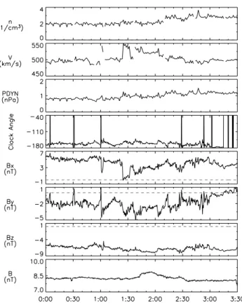
The upstream solar wind and interplanetary magnetic field (IMF) measurements in geocentric solar magnetospheric (GSM) coordinates from ACE are shown in Fig. 2. The data in Fig. 2 is already time-shifted by 54.4 min, which is ob-tained by matching the sudden northward turning of the IMF measured at both ACE and Cluster. The northward turning took place around 03:34:46 UT for Cluster 1 and 02:40:22 for ACE (not shown here since it is outside the interval of interest). From top to bottom, Fig. 2 shows the solar wind proton density, speed, dynamic pressure, IMF clock angle (defined as t an−1(By/Bz)), IMF Bx, By, Bzand |B|. During
these three and one-half hours, the average solar wind speed was about 500 km/s, the density was about 2.3 cm−3, the dy-namic pressure was 1.0 nPa and the average clock angle was
about −160◦. The IMF B
x was positive, and By and Bz
were both negative. Prior to this event, the IMF Bzhad been
mostly southward for about 17 h, which resulted in strong au-roral activity, indicating that the solar wind-magnetosphere-ionosphere coupling was effective.
3.3 Event overview
Overviews of the event are given in Figs. 3, 4 and 5. Fig-ure 3 contains the ion moment data (such as velocity, den-sity and temperature) in the context of the magnetic field for the whole three and one-half hour interval. The purpose of
YGSM XGSM XGSM ZGSM Figure 1 A B
Fig. 1. The trajectory and the configuration of the Cluster quartet during the event with regard to the magnetic fields in XGSM−ZGSM and XGSM−YGSM planes. The magnetic field
lines are derived from the T96 model using the solar wind and IMF conditions at the time. The green asterisks along the trajectory are the spacecraft position at 00:00, 00:10, 01:00, 01:30, 02:00, 02:30 and 03:00 UT, respectively. Also shown in Fig. 1 is the tetrahedron made up by the four spacecraft at 01:30 UT (for the purpose of clar-ity, the separation distance relative to C3 was multiplied by a factor of 5.0) with C1 in black, C2 in red, C3 in green and C4 in blue.
Figure 2
Fig. 2. The solar wind and IMF measurements in GSM from the ACE spacecraft. The time is shifted by 54.4 min to match the sud-den northward turning of the IMF measured at both the ACE and the four Cluster spacecraft. Notice the IMF Bzwas negative throughout
the whole interval. The IMF Bywas also negative.
this plot is to emphasize the long-lasting accelerated flows. Complementary to Figs. 3, 4 and 5 are two subsets of the event where both electron and ion energy-time spectrograms are shown. The regions traversed by the Cluster spacecraft
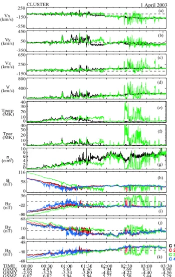
00:00 00:30 01:00 01:30 02:00 02:30 03:00 03:30 -68 -10 48 C 1 C 2 C 3 C 4 4.06 -2.92 6.07 4.87 -3.25 6.02 5.63 -3.54 5.94 6.36 -3.80 5.84 7.04 -4.02 5.72 7.69 -4.22 5.58 8.31 -4.40 5.44 8.90 -4.56 5.29 TIME GSMX GSMY GSMZ Bx (nT) -48 10 68 C 1 C 2 C 3 C 4 By (nT) -80 -22 36 C 1 C 2 C 3 C 4 Bz (nT) 0 58 116 C 1 C 2 C 3 C 4 B (nT) 0 2 4 6 8 10 C 1 C 2 C 3 C 4 n (c m-3 ) 0 10 20 30 40 C 1 C 2 C 3 C 4 Tpar (MK) 0 10 20 30 40 C 1 C 2 C 3 C 4 Tperp (MK) 0 400 800 C 1 C 2 C 3 C 4 V (km/s) CLUSTER -150 250 650 Vz (km/s) -350 50 450 Vy (km/s) -550 -150 250 Vx (km/s) (a) (b) (c) (d) (e) (f) (g) (h) (i) (j) (k) 1 April 2003 Figure 3
Fig. 3. The overview of the event showing the particle and the mag-netic field data. The top seven panels are the particle parameters obtained using HIA (only operative in C1 and C3). From top to bottom are the three components of the ion bulk velocity, its mag-nitude, the perpendicular and the parallel temperature, and the den-sity, respectively. The magnitude and the three components of the magnetic field for all of the four spacecraft are shown in the bottom four panels. The color scheme to represent the four spacecraft is the standard one: with C1 in black and C2 in red, and C3 in green and C4 in blue.
and the properties of each region are best seen from Figs. 4 and 5.
Shown in the top seven panels of Fig. 3 are ion measure-ments from the HIA instrumeasure-ments on C1 and C3 (only opera-tional on C1 and C3). The bottom four panels of Fig. 3 are the measurements of the magnetic field from the four space-craft. Figure 3a is the x-component of the ion bulk velocity and b, c, d show the y-, z-components and magnitude, re-spectively. The ion perpendicular and parallel temperatures are shown in Figs. 3e and f. Figure 3g is the ion density. The magnitude and the three components (x,y,z) of the magnetic field are shown in h, k, j and i, respectively.
The most noticeable feature in Fig. 3 is that accel-erated flows were detected during the time from about 00:50 UT to 3:20 UT, whenever Cluster encountered a mag-netopause/boundary crossing, indicating that magnetic re-connection can be continuous for many hours.
During the course of their outbound traversal from the plasma mantle poleward of the cusp, through the cusp, to the magnetopause boundary, and finally into the magnetosheath, the Cluster spacecraft encountered the magnetopause bound-ary numerous times. Mainly due to the motion of the mag-netopause, these encounters occurred in two general regions: (A) near the equator-edge of the northern cusp, where the open-closed field line boundary probably resides (roughly where A is in Fig. 1 and ∼00:50–01:40 UT in Fig. 3), and the magnetic shear between the magnetosheath-like region and the magnetospheric-like region was small; and (B) the dayside magnetopause boundary equatorward of the cusp (roughly where B is in Fig. 1 and ∼02:00–03:30 UT in Fig. 3), and the magnetic shear across the magnetopause was large (close to 180◦). Due to the specific configuration of the four spacecraft and the motion of the magnetopause bound-ary, C1, C2 and C4 had multiple crossings with the first type of magnetopause at different times, while C3 did not, as it was trailing the other three. For the same reason, when C3 crossed the second type of magnetopause multiple times, the other three spacecraft were mostly in the magnetosheath and had only a few partial or no encounters with the magne-topause.
Because HIA data are only available from C1 and C3, the overview of the first type of boundary crossings (low mag-netic shear) is better viewed using HIA data from C1 (see the shaded region in Fig. 4) and the overview of the second type of boundary crossings (high magnetic shear) is shown as the highlighted region in Fig. 5, using data from C3. Fig-ures 4 and 5 have the same format: from top to bottom, one sees the electron time spectrogram, the ion energy-time spectrogram, assuming that the ions are protons, the density in cm−3, the three components of the proton velocity in GSE (x in red, y in green and z in blue), the proton tem-perature (with the perpendicular temtem-perature in blue and the parallel temperature in magenta and the total temperature in black), and Bx, By, Bzin GSE and B, respectively. The
time-energy spectra of both ions and electrons (Figs. 4 and 5) of the event show that the four spacecraft traversed through dif-ferent plasma regions during the interval of 00:00–03:30 UT. These regions include: (1) the plasma mantle (from 00:00 UT to about 00:23 UT for C1 in Fig. 4), with a very small plasma density (∼0.2 cm−3); (2) the cusp (00:23–00:50 UT),
char-acterized by enhanced density (sometimes reaching to 1.0– 2.0 cm−3)of magnetosheath-like plasma; (3) the boundary plasma sheet (BPS, 00:50 UT ∼01:13 UT), with an obvious presence of energetic ions and electrons (10 keV above for ions and 1 keV above for electrons); (4) the magnetosheath region close to the magnetopause (01:55∼02:00 UT in Fig. 4 and 03:25–03:30 UT in Fig. 5), with the majority of elec-trons in the 50-200 eV range, and ions in the 40 eV−4000 eV range and an average ion density of a few cm−3; and (5)
C1
Plasma Mantle Cusp
BPS MP’xing Msh Energy eV 1.4 e+04 3.8 e+03 1 e+03 2.8 e+02 74 10 11 12 D e ne rgy flux 1/m 2/sr/s 10 10 10
Fig. 4. The overview of the boundary crossings with small mag-netic shear. The top panel is the electron energy-time spectrogram, the next four panels show the ion data from HIA and the bottom four panels are the magnetic field data. From top to bottom is the electron energy-time spectrogram, the ion energy-time spectro-gram, density, the three components of velocity in GSE coordinates with the x component in red, y in green and z in blue), the parallel (red) and the perpendicular (blue) temperature, the x component of the magnetic field in GSE-Bx, By, Bzand B, respectively. Notice
the different regions traversed by the spacecraft, as shown in the top panel.
the magnetopause boundary layers where the accelerated flows were observed. The first type of boundary layer is the interface between the polar cusp and the magnetosphere. The plasma within shows alternations between the BPS-like plasma and magnetosheath-like plasma (Fig. 4). The sec-ond type of boundary layer is the dayside magnetopause just equatorward of the cusp, i.e. the interface between the magnetosheath and the dayside magnetosphere. The plasma there oscillates between the magnetosheath and magneto-sphere proper (Fig. 5). Note that, prior to the highlighted region in Fig. 5, C3 was located in the magnetosheath, but had two excursions (at around 02:05 UT and 02:17 UT) into the magnetopause/boundary layer, as evidenced by both the
C3 Energy eV 1.4 e+04 3.8 e+03 1 e+03 2.8 e+02 74 10 11 12 D e ne rgy flux 1/m 2/sr/s 10 10 10
Fig. 5. The overview of the boundary crossings with large magnetic shear. Figure 5 has the same format as Fig. 4.
particle and the field parameters shown in Fig. 5. The mul-tiple magnetopause encounters of Fig. 5 show that through-out the whole interval, the motion and/or the structure of the magnetopause were rather complex.
4 Analyses of the accelerated flows and implications for continuous reconnection
4.1 Characteristics of the accelerated flows
The accelerated flows were observed at both types of magne-topause boundary crossings, one with a small magnetic shear and the other with a large magnetic shear. These flows ex-hibit the following common characteristics based on Figs. 4 and 5.
1. The accelerated flows had very large flow speed com-pared to the magnetosheath plasma, at times reach-ing ∼700 km/s (exceedreach-ing their adjacent magnetosheath flow speed by ∼550 km/s) and persisted for a long time - almost 3 h. The ion β in the magnetosheath was about 0.2–0.5 during the event. This low β value favors the
occurrence of accelerated flows as showed by Scurry et al. (1994a).
2. Whenever there was accelerated flow, there was a rota-tion or at least change in magnetic field.
3. Of all the observed high-speed jets, the peak of the flow speed occurred at the earthward edge (magnetospheric side) of the current layer (Gosling et al., 1986), as ex-pected (Sonnerup et al., 1995).
4. Within the accelerated flows, the ion density was usu-ally smaller than that observed in the adjacent mag-netosheath but slightly larger than that of the adjacent
magnetosphere. The temperatures within the
accel-erated flows were between the values of the magne-tosheath and the magnetosphere, but closer to those of the magnetosheath.
5. For most of the observed flows, the magnitude of the magnetic fields was roughly the same on both sides of the magnetopause, but it was greatly reduced within the magnetopause current layer. The presence of such field depressions is common in the magnetopause cur-rent layer and has been reported in other reconnection events (e.g. Paschmann et al., 1979; Gosling et al., 1986, 1990c, 1991; Phan et al., 2001, Mozer et al., 2002). 6. The accelerated flows were in the positive y and z
direc-tions, i.e. the plasma had duskward and northward ac-celeration, which agrees with the jet direction resulting from magnetic reconnection based upon the configura-tion of magnetic fields in the magnetosheath (negative
By and negative Bz). When By (IMF Bz negative) is
negative, the force pulls the plasma towards northeast in the Y-Z plane in the northern dawn quadrant and the opposite direction in the southern dusk quadrant (see the bottom panel of Fig. 1 in Gosling et al. (1990c)). 7. Flow reversals were observed throughout the event, i.e.
the y-component of the flow within both the high lati-tude boundary layer (magnetospheric side) and the mag-netopause current layer had the opposite sign (+Vy,
duskward) from that within the adjacent magnetosheath (-Vy, dawnward). The flow reversals in the y
compo-nent of the ion bulk velocity are the result of magnetic reconnection, as described in Gosling et al. (1990c).
Figure 6 illustrates the observed flow reversals (second panel,
Vy; the gaps are due to missing data) at the two types of
magnetopause crossings. The shaded areas of Fig. 6 high-light the magnetosheath region, where the y-component of the plasma, flow was opposite (negative Vy)to that within
the magnetopause and its earthward boundary layer (positive
Vy).
4.2 Fluid signature of reconnection - tangential stress bal-ance tests
In this section, we show quantitatively that the accelerated flows are reconnection jets by performing the tangential stress balance tests. First, using the tangential stress balance relation, we calculate the predicted velocity for extended intervals based on a single magnetosheath reference point. Then we show that the high-speed flows satisfy the Wal´en re-lation, which is often used as strong (if not incontrovertible) evidence that magnetic reconnection was occurring or had been occurring in the immediate past at the magnetopause.
During reconnection, the magnetopause consists of a ro-tational discontinuity (RD) (Levy et al., 1964). The tangen-tial stresses at an RD can lead to deceleration of the plasma as well as acceleration, depending upon the geometry of the external magnetic field and plasma flow. For an RD, ideal MHD predicts that the flow is Alfv´enic in the deHoffmann-Teller (HT) frame of reference (Hudson, 1970):
ρ(1 − α)=const. (1)
v − VH T= ±(1 − α)1/2B/(µ0ρ)1/2, (2)
where ρ is the total mass density and α≡(P||−P⊥)µ0/B2
is the pressure anisotropy factor (P|| and P⊥are the plasma
pressure parallel and perpendicular to B), v is the plasma ve-locity, VH T is the deHoffmann-Teller velocity, the motion of
the open flux tubes along the magnetopause resulting from the magnetic tension force (VH T=Et×Bn/Bn2, where Et is
the tangential electric field and Bn is the normal magnetic
field), and B is the magnetic field. The right-hand side of Eq. (2) represents the Alfv´en velocity. Equation (2) is also called the Wal´en relation.
4.2.1 Test using a single reference point
Before performing the Wal´en test, we will first show a quanti-tative evaluation of the agreement between the predicted and the observed high-speed flows at both types of boundaries based on a single magnetosheath reference point (Phan et al., 2004). From Eqs. (1) and (2), we can obtain the following relation:
1vpredicat ed=v2t−v1t=+(1−α1)1/2µ0ρ
−1/2
1
[B2t(1−α2)/(1−α1)−B1t] (3)
The positive sign was chosen because the Cluster spacecraft were above the potential reconnection site. Subscript “1” is used to represent the magnetosheath reference point and “2” is used to represent any other times for calculating the pre-dicted velocity. The results at the first type (low magnetic shear) of boundary crossing (using C1 data) are shown in Fig. 7 and those at the high-magnetic shear crossings (from C3 measurements) are shown in Fig. 8. For both Figs. 7 and 8, the top three panels are the time-shifted ACE data of the interplanetary magnetic field. The bottom three pan-els show the measured HIA (in black) and the predicted (in
C1 - flow reversal at 1st type of MP’xing C3 - flow reversal at 2nd type of MP’xing
Figure 6
Fig. 6. Flow reversals in the y component of the ion bulk flow are shown for two types of magnetopause crossings. The left and the right panels are for the first and second type of crossing respectively. The shaded regions in the plot are used to highlight the magnetosheath region where the flow has negative Vy, opposite to that of the magnetopause and its boundary layers.
red) velocity in boundary normal coordinates using the netopause model by Shue et al. (1997). For Fig. 7, the mag-netosheath reference point is at 01:41 UT (the dashed line). For the Fig. 8 calculation, the reference point is at 03:09 UT and is also marked by the dashed line in the plot. This test works best when the IMF condition is relatively steady. De-spite the somewhat varied IMF conditions and, therefore, the variations in the sheath magnetic field, Fig. 7 shows that the predicted velocity tracks the measured velocity well. Since the points at the beginning of the period are more than half an hour away from the reference point, the agreement is not per-fect. Figure 8 has the same format as Fig. 7, except that the green asterisks show the predicted velocity when the density is higher than 5 cm−3. By looking at the black and the red lines in Fig. 8, the first impression is that the agreement be-tween the measurements and the predicted values is not very good, especially at the beginning of the interval. If we look at Fig. 8 more carefully, however, we find that the disagree-ments occurred when C3 was either at the magnetosphere or at the inner part of the boundary layer, which is no longer an RD (Phan et al., 2001). The reconnection layer consists of an outer RD, followed by a region of uniform flow and field and then an inner slow mode expansion fan according to MHD models of dayside reconnection. This point can be
demon-strated by comparing the predicted velocity when the density is higher than 5 cm−3(about half of the magnetosheath
den-sity) and the measured velocity (the green asterisks and the black line in Fig. 8). The density condition applied here is to make sure that the comparison is made across the RD only. We can see that the agreement is improved. The slow ion sampling rate (a sample every 4 s) plus the additional missing data may contribute to the disagreement, as well. As men-tioned above, even though the IMF condition for this event was not very steady, the results displayed in Figs. 7 and 8 show that the high-speed flows are most likely the result of magnetic reconnection.
4.2.2 Wal´en relation test
The Wal´en relation states that in the deHoffmann-Teller (HT) frame, the flows are field-aligned and Alfv´enic. The HT frame for a set of plasma measurements can be found by minimizing the mean square of the convection electric field, D(v)=<|(v−VH T×B|2> (Sonnerup et al., 1987). In the
HT frame, the convection electric field ideally should
van-ish. The velocity v at which D(v) is a minimum is the
deHoffmann-Teller velocity, VH T. The ratio of DH T/D0
01:00
Figure 7 Fig. 7. Comparison between the predicted ion bulk flow velocity and the data for the first type of boundary crossing with small mag-netic shear. The prediction used a single magnetosheath point as the reference point. The top three panels are the three components of IMF in GSM. The bottom three panels are the velocity comparison of the three components. The theoretical predication is in red and the data is in black.
used as a measure of the quality of the HT frame. For the existence of a good HT frame, the ratio should be very small ( 1).
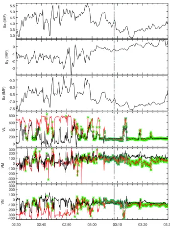
Two examples of the Wal´en relation test are shown in Fig. 9. The examples were selected arbitrarily; the left-hand one showing the Wal´en test of the accelerated flows at the low magnetic shear boundary crossing, and the right-hand one showing the test for the flows at the high magnetic shear crossing. The data interval for the first type (low shear) of boundary crossing analysis is 01:34:30 UT–01:36:00 UT and the reference time is at 01:41:00. The interval for the sec-ond type (high shear) of boundary crossing is 02:55:30 UT– 02:55:50 UT and the reference time is 03:09 UT. The positive slopes of the regression line in Fig. 9 imply that the normal magnetic field points earthward (i.e. BN<0) (e.g. Sonnerup
et al., 1981), consistent with a reconnection X-line below the spacecraft. The colors in the plots are used to indicate x (in black), y (red), and z (blue) components, respectively. For the first example, VH T is (17.3, 62.2, 300.5) km/s in
GSM coordinates. For the second example, VH T is (−268.9, −65.8, 290.0) km/s in GSM. The ratio of DH T/D0 is 0.080
Figure 8
Fig. 8. Comparison between the predicted ion bulk flow velocity and the data for the second type of boundary crossing with large magnetic shear. It has a similar format as Fig. 7, except for the green asterisks, which show the theoretical calculation when the density is above 5 cm−3, to avoid an inappropriate comparison in the region inside the magnetopause which is no longer a rotational discontinuity.
for the first case and 0.088 for the second case. When
vm×Bm is plotted against VH T×Bm (Figs. 9a and c), the
best fit has a slope of 1.00 and a correlation coefficient 0.95 for the first case and a slope of 1.00 and a correlation co-efficient 0.99 for the second case, indicating that a good HT frame exists for both crossings. Figures 9b and d show that in the HT frame, the flow is 93% of the Alfv´en velocity, for the first example, with a correlation coefficient of 0.98, and the flow is 83% of the Alfv´en velocity, for the second example, with a correlation coefficient 0.94. These test results indi-cate that both the speed and the direction of the observed ion bulk flows are in good agreement with the theoretical predic-tion, even with the assumption of a 1-D magnetopause and the fact that HIA ion moments are computed assuming that all ions are H+. The O+ density in the jet is about 0.02– 0.03 cm−3(<0.5% of the H+ density in the magnetosheath), which is similar to that in the magnetosphere. The presence of heavy ions (such as O+) will decrease the Alfv´en velocity, and therefore will result in a larger slope in the Wal´en test plot (such as Figs. 9b and d). But the O+ density here is too small to affect the Wal´en relation.
Figure 9
(a)
(b)
(c)
(d)
Fig. 9. The Wal´en relation test results for both types of magnetopause crossings. The two intervals (C1: 01:34:30–01:36:00 UT and C3: 02:55:30–02:55:50 UT) are randomly chosen with the left two panels showing the result for the first type and the right two panels showing the result for the second type. For each type, the top panel is the result of finding the deHoffmann Teller (HT) frame and the bottom panel shows the fitting result of the measured velocity in the HT frame versus the Alfv´en velocity.
The tests described above show that the long-lasting ac-celerated flows observed on 1 April 2003 are caused by re-connection, implying that magnetic reconnection took place continuously over a period of 3 h. Because the magnetopause (MP) is a relatively thin layer with a single spacecraft one can never be certain whether reconnection is operating continu-ously or not, even though the spacecraft could have multi-ple encounters with MP and observe high-speed jets for each of the crossings. One can potentially argue that when the spacecraft is not in the MP, the reconnection stops. The four Cluster spacecraft not only extend the potential encounter time with the MP, but also provide more information for de-termining whether the reconnection is continuous. For this event, the configuration of the four spacecraft was such that C1, C2 and C4 were in a plane that was close to tangential to the MP, while C3 lagged behind. For the first type (low magnetic shear) of boundary crossing (during the interval of 00:30 UT–02:00 UT), the boundary crossing happened al-most continuously because of the spatial arrangement of C1,
C2 and C4. The HIA of C1 and CODIF of C4 (not shown here) show the observation of accelerated flows whenever either of them was in the MP/boundary layer. The lack of ion data from C2 may be compensated for by the deduction from the similar features of the four spacecraft magnetic field measurements. All of these points argue strongly that recon-nection was operating continuously for the interval. For the second type (high magnetic shear) of MP/boundary crossing (2:00 UT to 3:30 UT), during which C1, C2 and C4 were already in the magnetosheath (most of the time), the large separation between C3 and the other spacecraft shows that C3 is the major spacecraft which detected the high-speed jets when it had multiple MP crossings during this interval. During 2:25–2:38 UT, however, because of the motion of the MP (which most likely resulted from reconnection because the solar wind dynamic pressure was weak and relatively sta-ble), C1, C2 and C4 encountered the boundary layer from the magnetosheath side at slightly different times and observed accelerated flows (seen from HIA data of C1 and CODIF of
(a) (b) (c) (d) (e) (f) 01:28:04.914 01:29:17.442 01:29:54.211 01:30:06.173 01:30:13.974 01:31:14.420 10 11 12 D ener gy flux 1/m 2 /sr/s eV eV
Fig. 10. Electron velocity distribution obtained from PEACE during an interval of the first type boundary crossing. Also shown is the magnetic field data during the interval. The timing of the distributions is indicated in the plot.
C4). In general, the data from all of the spacecraft, combined with the IMF condition at the time, provide good evidence that the reconnection was continuous for about 3 h.
4.3 Kinetic signatures of reconnection during accelerated
flows – Plasma distributions
We examined the kinetic signatures of reconnection using the electron and ion velocity distributions; first, we show an ex-ample related to the first type of boundary crossing, followed by the particle distributions of the second type of boundary crossing.
4.3.1 Electron distributions
Figure 10 shows the electron velocity distribution plots (with a 4-s cadence and 118-ms accumulation time), obtained us-ing both the LEEA (Low Energy Electron Analyzer) and HEEA (High Energy Electron Analyzer) of the PEACE in-strument during a cusp-magnetosphere interface crossing of C3 (01:28–01:32 UT). LEEA covers the energy range
of 0.7 eV–1 keV, HEEA covers the energy range of 30 eV– 26 keV and they are placed on opposite sides of the space-craft. The corresponding magnetic field profile is also shown for every distribution, as a reference. Shown on top of each distribution is their starting time in UT. The distribution plots are shown in the V−θ plane, referenced to the instantaneous high-resolution magnetic field. V is the magnitude of the electron velocity, shown here in the unit of the electron cen-tral energy in eV and θ is the pitch angle. The magnetic field direction lies in the vertical axis, with the upper half having a 0◦pitch angle and the lower half having a 180◦pitch angle. The left side of each distribution shows the HEEA data and the right side shows the LEEA data. It should be mentioned that this format assumes that the distributions are gyrotropic. On each of the distributions, the four white circles from the inside out are 50 eV, 200 eV, 1 keV and 5 keV, respectively. The color in the distribution plots is used to indicate the in-tensity of the differential energy flux (1/m2/s/sr).
The distribution function in both panels 10a and b shows counter-streaming fluxes of electrons in the low-energy range
(∼100 eV) and the co-existence of a high-energy population (up to ∼10 keV) centered at the 90◦pitch angle. The
counter-streaming fluxes of the electrons in the low-energy range in 10a and b do not necessarily imply that C3 was on the closed field lines at these times; rather the distributions were most likely the incoming (∼100 eV) and mirrored magnetosheath electrons on an open field line due to their low energy range. The co-existing population of magnetospheric origin at 90◦ pitch angle, together with the absence of the field-aligned magnetospheric electrons, may indicate that at these times C3 was on open field lines at the high-latitude boundary layer.
Figure 10c was obtained at the magnetospheric edge of the magnetopause current layer. The distribution was again composed of two populations, the accelerated magnetosheath electron population and the energetic magnetospheric elec-trons to above 20 keV, which were peaked at 90◦. The
ab-sence of the field-aligned electrons again indicates an open field line topology, where the field-aligned energetic elec-trons escaped. Figure 10d and 10e show velocity distribu-tions in the magnetopause current layer where the majority of the electrons are of magnetosheath origin. The tosheath electrons were heated dramatically in the magne-topause current layer and were moving towards the Earth (unheated magnetosheath electrons were mostly below the 100 eV range originally, but here we see them heated to 200– 300 eV, on average). The observed electron heating in the magnetopause current layer agrees with previous findings by Fuselier et al. (1995) for the low-latitude subsolar region. There were fewer magnetospheric electrons at these times (Fig. 10d and e compared with Fig. 10c). The reason for the missing data at some of the pitch angles in Fig. 10d is due to the fact that the direction of B moved significantly dur-ing the 4-s spin, so that some directions sampled durdur-ing the 118-ms accumulation of the slice of the distributions were no longer being sampled with respect to the instantaneous B. Figure 10f is the distribution at the high latitude boundary layer with its distribution similar to Figs. 10a and b, with the exception that its low energy part is more isotropic.
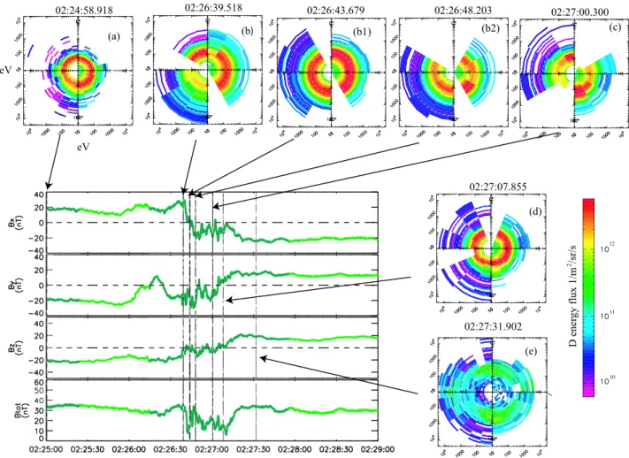
Figure 11 is in the same format as Fig. 10 but for a bound-ary crossing of the second type, i.e. the magnetopause with a large magnetic shear. Displayed in Fig. 11 are the mag-netic field data from 02:25:00 UT to 02:29:00 UT and the electron distributions in five distinct regions: (a) in the mag-netosheath, (b) at the magnetosheath edge of the MP current layer, (c) inside the MP current layer, (d) at the earthward edge (magnetospheric side) of the MP current layer, and (e) in the magnetospheric region.
As references, Figs. 11a and e show the distributions of typical cold magnetosheath electrons and tenuous hot
mag-netospheric electron, respectively. The mixture of
mag-netospheric and magnetosheath electrons and the heated, earthward-moving magnetosheath electron population in b, c and d indicate the interconnection of the magnetic field lines of the two regions. Figures 11b1 and b2 are used to show the evolution of the electrons in the current layer. The times in Figs. 11b, b1 and b2 are 4 s apart. We can see the dramatic
heating of the magnetosheath electrons at all of these times. Again, the incomplete coverage of the pitch angle in Figs. 11 b, b1, b2, c and d reflects the rapid changing magnetic field at those times.
Our observations show that heating of the magnetosheath electrons is a common feature in the magnetopause current layer for both types of magnetopause crossings. These obser-vations also favor the view that magnetic reconnection was operating at the time.
4.3.2 Ion distributions
Figures 12 and 13 show the ion velocity distributions ob-tained from the HIA instrument of C3 in the (V⊥,V||)plane
for two types of MP crossings, respectively. The time inter-val of Fig. 12 is same as that of Fig. 10 and the time interinter-val of Fig. 13 is the same as in Fig. 11. V⊥is in the (V×B)×B
direction (V is the bulk velocity) and the distributions are col-lected on board over 12 s. The two-dimensional distributions are plotted in a reference frame moving with the perpendicu-lar bulk velocity. Shown in Fig. 12 are the distributions at the first type of boundary crossing with Figs. 12a and c obtained in the high-latitude boundary layer and Fig. 12b in the MP current layer. When the magnetic shear across the MP is low, we see the mixture of magnetosheath and magnetospheric ions for all three distributions, indicating the open-field line topology. The lack of field-aligned high-energy ions of mag-netospheric origin in Figs. 12a and c indicates that they may have escaped along the open-field lines, consistent with the electron distribution in Fig. 10. Meanwhile, Fig. 12b shows that in the magnetopause current layer, the high-energy ions were moving outward along the field line (anti-parallel to B) and the magnetosheath ions were accelerated.
Figure 13 shows the distributions at a high magnetic shear MP crossing in the magnetosheath region (Fig. 13a), in the MP current layer (Figs. 13b, c and d) and in the magneto-sphere region (Fig. 13e). Of these, 13b is closer to the mag-netosheath edge of the current layer, Fig. 13c is in the heart of the MP current layer and Fig. 13d is located at the magneto-spheric side of the MP current layer. Similar to the electron distributions during the same interval, the ion distributions here show a mixture of the two populations, as well as strong ion acceleration (see Figs. 13b, c and d). The magnetosheath ions were mostly below 5 keV (corresponding roughly to the 1000 km/s in the plots for H+) while for the high-energy magnetospheric population, ions below 1.25 keV were absent (see Fig. 13e).
The theory of magnetic reconnection predicts the exis-tence of the D-shaped magnetosheath ion distribution at the MP (Cowley, 1982), and it has been reported widely in the literature (e.g. Gosling et al., 1990a; Fuselier et al., 1991; Smith and Rodgers, 1991; Bauer et al., 1998; Phan et al., 2001). However, D-shaped ion distribution was not observed during our two examples. One could argue that the b, c and d distributions in Fig. 13 are D-shaped, considering that the magnetic field was highly variable and the distribution was averaged over 12 s. But the fluid and the kinetic signatures at
(a) (b) (b1) (b2) (c) (d) (e) 02:27:31.902 02:27:07.855 02:27:00.300 02:26:48.203 02:26:43.679 02:26:39.518 02:24:58.918 Figure 11 10 11 12 D ener gy flux 1/m 2/sr/s eV eV
Fig. 11. Electron velocity distribution function during an interval of the second type boundary crossing with large magnetic shear.
the MP do not always appear together, as also reported pre-viously. More often than not, the fluid signatures (Alfv´enic flows) are observed without the D-shaped ion distributions, and vice versa (see Bauer et al. (1998)). For further ex-pansion of this, distributions of the two intervals shown in Fig. 10 (during which the fluid signature had excellent agree-ment with the Wal´en relation) were also carefully studied, and no D-shaped distributions were found. The absence of the D-shaped ion distributions at and around the MP, in spite of the excellent agreement with the Wal´en relation, was also reported by Phan et al. (2004). The presence of magneto-spheric ions in the magnetosheath side of the MP current layer and the magnetosheath ions earthward of the MP cur-rent layer, however, shows that there was transmission of ions across the MP boundary, which is one of the kinetic effects of reconnection.
Another interesting feature to note is that the ion distribu-tions in Figs. 13b, c and d were non-gyrotropic (asymmetric about the x-axis), which probably resulted from magnetic re-connection. The non-gyrotropic distribution is a source of free energy that can excite instabilities. The significance of the non-gytropic ion distributions in the vicinity of the mag-netopause requires further investigation.
4.4 Summary of the analyses of the long-lasting high speed plasma jets
The analyses of the prolonged interval of accelerated plasma flows observed at/around the MP and its boundary layers im-ply that they were most likely caused by magnetic reconnec-tion, as was demonstrated from both fluid and kinetic per-spectives. The long-lasting nature of the high-speed flows and their detection by multiple spacecraft also argue strongly that reconnection was operating continuously for more than 3 h. Both the magnetic field and the particle data help reveal many characteristics of the magnetopause current layer. In-side the MP current layer, magnetic field is highly variable and the magnetic field depression is a common feature. We also find that both electrons and ions of magnetosheath ori-gin become heated in the MP current layer, mostly as a result of magnetic reconnection in this case.
5 Discussion
To date, the evidence for magnetic reconnection at the mag-netopause and its subsequent consequences on the global dynamics of the magnetosphere have been widely reported.
-2000 -1000 0 1000 2000 01:29:25 - 01:29:37 V|| V⊥0 θB 147. φB -152. v: [-21.0, 74.1, 7.5] |v|: [77.4] v⊥: [-28.1, 70.3, -5.2] v||: [-15.1] B: [-15.11, -8.02, -26.84] x z x y
range: [7.9e-29, 1.3e-21] 01:30:02 - 01:30:14
V|| V⊥0 θB 113. φB -163. v: [-3.4, 208.6, -96.4] |v|: [229.8] v⊥: [-17.2, 204.3, -102.7] v||: [-15.7] B: [-24.95, -7.80, -11.33] x z x y range: [7.8e-29, 2.3e-21]
ninf: [0.80, 0.28, -0.53] -2000 -1000 0 1000 2000 01:31:14 - 01:31:26 θB 148. φB -154. v: [17.0, 91.3, -7.3] |v|: [93.1] v⊥: [6.0, 85.8, -27.1] v||: [-23.3] B: [-13.81, -6.87, -24.79] x z x y range: [7.8e-29, 7.6e-22]
-2000 -1000 0 1000 2000 -2000 -1000 0 1000 2000 -2000 -1000 0 1000 2000 -2000 -1000 0 1000 2000 (a) (b) (c) (a) (b) (c) -2 8 -27 -2 6 -25 -24 -23 -22 log 10 (df/s 3cm -6)
Fig. 12. Ion velocity distribution from HIA during the same interval as shown in Fig. 10, which is of the first type of boundary crossing. The resolution of these distributions is 12 s. The starting time of each distribution is indicated in the magnetic field data.
However, there are still many unanswered questions, includ-ing the nature of the physical processes that lead to an initial breakdown; which controls where and when reconnection takes place and at what rate; and which controls the cessa-tion and the temporal behavior of the reconneccessa-tion once it is initiated (continuous or intermittent). Because signatures of reconnection (e.g. plasma jets) are localized in the thin magnetopause and can therefore only be observed for sev-eral minutes as a spacecraft traverses the layer, only a limited number of reports have shown evidence of continuous recon-nection (Gosling et al., 1982; Phan et al., 2004; Retin`o et al., 2005; and Frey et al., 2003).
The fact that continuous reconnection can take place un-der both southward (e.g. Phan et al., 2004 and this paper) and northward IMF (e.g. Retin`o et al., 2005; Frey et al., 2003) conditions shows that the temporal nature of reconnection is independent of the polarity of IMF and is more likely trolled by externally driven processes or by changes in con-ditions internal to the magnetosphere.
In contrast to continuous reconnection, intermittent or bursty reconnection has been widely reported in the solar atmosphere where eruptive processes are time-limited (e.g. Priest and Forbes, 2002), at the magnetopause in the form of pulsed reconnection (e.g. Farrugia et al., 1998; Lockwood et al., 1998, 2001; Sandholt et al., 2000; Milan et al., 1999), in flux transfer events (FTEs) (e.g. Russell and Elphic, 1979), and in the magnetotail, where the observation of bursty bulk flows, potentially the analogue of FTEs at dayside, were ob-served.
Recent observation of continuous reconnection by IMAGE and Cluster calls for a better understanding of which pro-cesses/conditions control the different temporal behaviors of magnetic reconnection. How the temporal behavior of recon-nection affects the energy input to the magnetosphere from the solar wind is not fully understood, nor do we know which process, continuous reconnection or bursty reconnection, is more efficient in terms of mass, energy and momentum
Figure 13 ninf: [0.48, -0.36, -0.80] 02:25:02 - 02:25:14 θB 107. φB -58. v: [-113.6, 43.4, 95.9] |v|: [154.8] v⊥: [-51.5, -54.4, 61.0] v||: [-121.0] B: [17.69, -27.85, -9.93] x z x y
range: [7.8e-29, 2.0e-21]
-2000 -1000 0 1000 2000 -2000 -1000 0 1000 2000 ninf: [0.88, -0.20, -0.43] -2000 -1000 0 1000 2000 -2000 -1000 0 1000 2000 02:26:50 - 02:27:02 θB 81. φB -136. v: [-368.2, 233.8, 267.2] |v|: [511.5] v⊥: [-268.1, 331.3, 245.0] v||: [141.5] B: [-10.84, -10.55, 2.41] x z x y
range: [7.8e-29, 2.4e-21]
ninf: [-0.45, 0.27, -0.85] ninf: [-0.67, -0.17, -0.72] -2000 -1000 0 1000 2000 02:27:02 - 02:27:15 θB 81. φB 133. v: [-345.2, 265.6, 244.2] |v|: [499.4] v⊥: [-30.9, -67.3, 169.3] v||: [463.9] B: [-9.18, 9.72, 2.19] x z x y
range: [7.8e-29, 2.2e-21]
ninf: [0.72, 0.59, 0.37] -2000 -1000 0 1000 2000 02:27:15 - 02:27:27 V|| V⊥0 θB 73. φB 131. v: [-210.3, 211.7, 174.1] |v|: [345.4] v⊥: [0.4, -30.3, 74.6] v||: [335.9] B: [-18.88, 21.70, 8.92] x z x y
range: [7.8e-29, 2.4e-21]
ninf: [0.78, 0.58, 0.23] -2000 -1000 0 1000 2000 02:27:39 - 02:27:51 θB 79. φB 139. v: [-13.5, 57.0, 57.6] |v|: [82.2] v⊥: [29.5, 20.1, 46.2] v||: [57.9] B: [-22.74, 19.51, 6.05] x z x y
range: [7.8e-29, 6.6e-21]
ninf: [0.44, 0.69, -0.58] (a) (a) (b) (c) (d) (e) (e) (d) (c) (b)
Fig. 13. Ion velocity distribution from HIA during the same interval as shown in Fig. 11, which is of the second type of boundary crossing with large magnetic shear.
physical quantities is another challenge. Answering these questions requires continuous observation of reconnection signatures at the magnetopause, which, at present, are not generally available. Although using ionospheric signatures of reconnection to remotely probe the reconnection charac-teristics at the magnetopause can serve as an important tool, it too has its own limitations, including a requirement for ac-curate field line tracing.
A striking feature of this event is that it had very high cou-pling efficiency in terms of the percentage of solar wind en-ergy being transferred to the magnetosphere-ionosphere (MI) system. The coupling efficiency is defined as the ratio of total energy deposited in the MI system (including total en-ergy of ring current, auroral precipitation, Joule heating and energy in the magnetotail) to the total available solar wind kinetic energy (Østgaard and Tanskanen, 2003). If we use the ε parameter (Akasofu, 1981) (the semi-empirical param-eter of the solar wind energy input to the magnetosphere due to dayside reconnection) as a proxy for the total MI energy, the coupling efficiency is about 32.3% if the scale length l0is
taken as 10 REand would be about 16% if l0is taken as 7 RE.
Even the 16% number is very large for the solar wind and
MI coupling, when normally considering the coupling coef-ficient is below 1% (Østgaard and Tanskanen, 2003). The large auroral index AE during the event is another indication of the strong coupling between the solar wind, the Earth’s magnetosphere, and the ionosphere.
6 Summary
A prolonged interval of accelerated plasma flows at high lat-itude near the northern cusp is studied in detail here. The event took place during 00:00–03:30 UT on 1 April 2003 while Cluster traveled outbound. Besides the long-lasting nature of the accelerated flows, Cluster observed high-speed flows at two different types of MP crossings, one of which had small magnetic shear and the other very large magnetic shear across the MP. The former was at a higher latitude (cusp-magnetosheath interface) than the latter (high-latitude dayside magnetopause). Observations of the event strongly suggest that magnetic reconnection, although time varying, can occur at various locations over a three-hour interval. The
key observations and interpretations can be summarized as follows:
1. The accelerated flows at the magnetopause/boundary layers had very large flow speed, at times reaching 700 km/s (exceeding their adjacent magnetosheath flow speed by ∼550 km/s) and they persisted for almost 3 hours. Whenever there was accelerated flow, there was magnetic field rotation or at least variations associated with it.
2. Flow reversals of the y-component of the ion bulk ve-locity were observed throughout the event (with neg-ative Vy in the magnetosheath and positive Vy for the
accelerated flows at the magnetopause and its bound-ary layers), which indicates strong acceleration from the magnetic tension force due to reconnection.
3. Accelerated flows were observed at most of the mag-netopause crossings. The speed and direction of two randomly selected magnetopause crossings are in excel-lent agreement with the 1-D model of the reconnecting magnetopause. The accelerated flows observed from the multiple spacecraft during the three and one-half hour interval support the interpretation of continuous recon-nection.
4. The persistent north-duskward flow throughout the three and half-hour interval implies that the reconnec-tion site remains southward of the spacecraft at all times. This event shows that magnetic reconnection was in large part controlled by the IMF. However, the obser-vations here cannot pinpoint whether it is component or anti-parallel reconnection that was at work because both theories would give similar observable features given the spacecraft’s location and the IMF direction (mostly southward).
5. Plasma jets were observed at two types of magne-topause crossings: one with small magnetic shear and the other with large magnetic shear. This should not be taken as evidence for component reconnection or for antiparallel reconnection, since it is the shear at the X-line, not at the local magnetopause, that matters. The high-speed jets observed at both types of magnetopause crossings most likely resulted from the same reconnec-tion site below the spacecraft.
6. Both electron and ion 3-D velocity distributions show that the plasma was heated at the magne-topause/boundary. Particle signatures resulted from connection, such as transmission of plasmas of both re-gions across the magnetopause, and the open field-line topology can be inferred. However, D-shaped (with the low energy cutoff at the deHoffmann-Teller velocity parallel to the magnetic field) ion distributions were not found even when the fluid features were in good agree-ment with the Wal´en relation. Why D-shaped ion dis-tribution occurs in some events and not in others is not well understood.
Acknowledgements. The authors want to thank all of those who
have made the Cluster mission a success. Suggestions from T. Phan are gratefully acknowledged. We would also like to thank the ref-erees for their helpful comments. The work was carried out while Y. Zheng held an NRC Resident Research Associate (RRA) fellow-ship.
Topical Editor T. Pulkkinen thanks I. Wild and another referee for their help in evaluating this paper
References
Aggson, T. L., Gambardella, P. J., and Maynard, N. C.: Electric field measurements at the magnetopause, 1, Observation of large convective velocities at rotational magnetopause discontinuities, J. Geophys. Res., 88, 10 000–10 010, 1983.
Akasofu, S.-I.: Energy coupling between the solar wind and the magnetosphere, Space Sci. Rev., 28, 121–190, 1981.
Arnoldy, R. L.: Signature in the interplanetary medium for sub-storms, J. Geophys. Res., 76, 5189–5201, 1971.
Balogh, A., Carr, C. M., Acu˜na, M. H., Dunlop, M. W., Beek, T. J., Brown, P., Fornac¸on, H., Georgescu, E., Glassmeier, K.-H., Harris, J., Musmann, G., Oddy, T., and Schwingerschuh, K.: The Cluster magnetic field investigation: Overview of in-flight performance and initial results, Ann. Geophys., 19, 1207–1217, 2001,
SRef-ID: 1432-0576/ag/2001-19-1207.
Bauer, T. M., Paschmann, G., Sckopke, N., Baumjohann, W., Treumann, R. A., and Phan, T. D.: AMPTE-IRM observations of particle and fields at the dayside low-latitude magnetopause, Geospace Mass and Energy Flow: Results from the International Solar-Terrestrial Physics Program, (Eds.) Horwitz, J. L., Gal-lagher, D. L., and Peterson, W. K., Geophysical Monograph, 104, 51–72, 1998.
Cowley, S. W. H.: The causes of convection in the Earth’s magne-tosphere: A review of developments during the IMS, Rev. Geo-phys. Space Phys., 20, 531–565, 1982.
Dungey, J. W.: Interplanetary field and the auroral zones, Phys. Rev. Lett. 6, 47, 1961.
Fairfield, D. H. and Cahill, L. J. Jr.: Transition region magnetic field and polar magnetic disturbances, J. Geophys. Res., 71, 155–169, 1966.
Farrugia, C. J., Sandholt, P. E., Denig, W. F., and Torbert, R. B.: Observation of a correspondence between poleward moving au-roral forms and stepped cusp ion precipitation, J. Geophys. Res., 103, 9309–9315, 1998.
Frey, H. U., Phan T. D., Fuselier, S. A., and Mende, S. B.: Continu-ous magnetic reconnection at Earth’s magnetopause, Nature 426, 533–537, 2003.
Fuselier, S. A., Klumpar, D. M., and Shelley, E. G.: Ion reflec-tion and transmission during reconnecreflec-tion at the Earth’s subsolar magnetopause, Geophys. Res. Lett., 18, 139–142, 1991. Fuselier, S. A.: Kinetic aspects of reconnection at the
magne-topause, in: Physics of the magnemagne-topause, Geophys. Monogr. Ser., Vol. 90, (Eds.) Song, P., Sonnerup, B. U. ¨O., and Thom-sen, M. F., AGU, Washington, D. C., 181–187, 1995.
Fuselier, S. A., Trattner, K. H., and Petrinec, S. M.: Cusp observa-tions of high and low-latitude reconnection for northward inter-planetary magnetic field, J. Geophys. Res., 105, 253–266, 2000. Gosling, J. T., Asbridge, J. R., Bame, S. J., Feldman, W. C., Paschmann, G., Sckopke, N., and Russell C. T.: Evidence for
quasi-stationary reconnection at the dayside magnetopause, J. Geophys. Res, 87, 2147–2158, 1982.
Gosling, J. T., Thomsen, M. F., Bame, S. J., and Russell C. T.: Ac-celerated flows at the near-tail magnetopause, J. Geophys. Res., 91, 3029–3041, 1986.
Gosling, J. T., Thomsen, M. F., Bame, S. J., Elphic, R. C., and Russell, C. T.: The electron edge of the low latitude boundary layer during accelerated flow events, Geophys. Res., Lett., 17, 1833–1836, 1990a.
Gosling, J. T., Thomsen, M. F., Bame, S. J., Elphic, R. C., and Russell, C. T.: Cold ion beams in the low latitude boundary layer during accelerated flow events, Geophys. Res. Lett., 17, 2245– 2248, 1990b.
Gosling, J. T., Thomsen, M. F., Bame, S. J., Elphic, R. C., and Rus-sell, C. T.: Plasma flow reversals at the dayside magnetopause and the origin of asymmetric polar cap convection, J. Geophys. Res., 95, 8073–8084, 1990c.
Gosling, J. T., Thomsen, M. F., Bame, S. J., Elphic, R. C., and Russell, C. T.: Observations of reconnection of interplanetary and lobe magnetic field lines at the high-latitude magnetopause, J. Geophys. Res., 96, 14 097–14 106, 1991.
Gustafsson, G., Bostr¨om, R., Holback, B., Holmgren, G., Lundgren, A., Stasiewicw, K., ˚Ahl`en, L., Mozer, F. S., Pankow, D., Harvey, P., Ulrich, R., Pedersen, A., Schmidt, R., Butler, A., Fransen, A. W. C., Klinge, D., Thomsen, M., F¨althammar, C.-G., Lindqvist, P.-A., Christenson, S., Holtet, J., Lybekk, B., Sten, T. A., Tanske-nen, P., LappalaiTanske-nen, K., and Wygant, J: The electric field and wave experiment for the Cluster Mission, Space Sci. Rev., 79, 137–156, 1997.
Hudson, P. D.: Discontinuities in an anisotropic plasma and their identification in the solar wind, Planet. Space. Sci., 18, 1611– 1622, 1970.
Johnstone, A. D., Alsop, C., Burge, S., Carter P. J., Coates, A. J., Coker, A. J., Fazakerley, A. N., Grande, M., Gowen, R. A., Gur-giolo, C., Hancock, B. K., Narheim, B., A. Preece, A., Sheather, P. H, Winningham, J. D., and Woodliffe, R. D.: Peace: A Plasma Electron and Current Experiment, Space Sci. Rev. 79, 351–398, 1997.
Levy, R. H., Petschek, H. E., and Siscoe, G. L.: Aerodynamic as-pects of the magnetospheric flow, AIAA J. 2, 2065–2076, 1964. Lockwood, M., Davis, C. J., Onsager, T. J., and Scudder, J. D.:
Modeling signatures of pulsed magnetopause reconnection in cusp ion dispersion signatures seen at middle altitudes. Geophys. Res. Lett., 25, 591–594, 1998.
Lockwood, M., Milan, S. E., Onsager, T., Perry, C. H., Scudder, J. A., Russell, C. T., and Brittnacher, M.: Cusp ion steps, field-aligned currents and poleward moving auroral forms, J. Geophys. Res., 106, 29 555–29 569, 2001.
McComas, D. J., Bame, S. J., Barber, P., Fieldman, W. C., Phillips, J. L., and Riley, P.: Solar wind electron, proton, and alpha mon-itor (SWEPAM) on the Advanced Composition Explorer, Space Sci. Rev., 86, 563–612, 1998.
Milan, S. E., Lester, M., Greenwald, R. A., and Sofko, G.: The iono-spheric signature of transient dayside reconnection and the asso-ciated pulsed convection return flow, Ann. Geophys., 17, 1166– 1171, 1999,
SRef-ID: 1432-0576/ag/1999-17-1166.
Mozer, F. S., Bale, S. D., and Phan, T. D.: Evidence of diffusion regions at a subsolar magnetopause crossing, Phys. Rev. Lett., 89, No. 1, 015002(4), 2002.
Østgaard, N. and Tanskanen, E.: Energetics of isolated and stormtime substorms, in: Disturbances in Geospace:
The Storm-Substorm Relationship, Geophys. Monogr., 142, doi:10.1029/142GM14, 2003.
Paschmann, G., Sonnerup, B. U. ¨O., Papamastorakis, I., Sckopke, N., Haerendel, G., Bame, S. J., Asbridge, J. R., Gosling, J. T., Russell, C. T., and Elphic, R. C.: Plasma acceleration at the Earth’s magnetopause, Evidence for magnetic reconnection, Na-ture, 282, 243–246, 1979.
Paschmann, G., Papamastorakis, I., Baumjohann, W., Sckopke, N., Carlson, C. W., B. U. ¨O. Sonnerup, B. U. ¨O., and L¨uhr, H.: The magnetopause for large magnetic shear, AMPTE/IRM observa-tions, J. Geophys. Res., 91, 11/,099–11/,119, 1986.
Phan, T. D., Paschmann, G., and Sonnerup, B. U. ¨O.: Low-latitude dayside magnetopause and boundary layer for high magnetic shear 2. Occurrence of magnetic reconnection, J. Geophys. Res., 101, 7871–7828, 1996.
Phan, T. D., Kistler, L. M., Klecker, B., Haerendel, G., Paschmann, G., Sonnerup, B. U. ¨O., Baumjohann, W., Bavassano-Cattaneo, M. B., Carlson, C. W., DiLellis, A. M., Fornacon, K.-H., Frank, L. A., Fujimoto, M., Georgescu, E., Kokubun, S., Moebius, E., Mukai, T., Øieroset, M., Paterson, W. R., and Reme, H.: Ex-tended magnetic reconnection at the Earth’s magnetopause from detection of bi-directional jets, Nature 404, 848–850, 2000. Phan, T. D., Sonnerup, B. U. ¨O., and Lin, R. P.: Fluid and kinetics
signatures of reconnection at the dawn tail magnetopause: Wind observations, J. Geophys. Res., 106A11, 25 489–25 501, 2001. Phan, T., Frey, H. U., Frey, S., Peticolas, L., Fuselier, S., Carlson,
C., R`eme, H., Bosqued, J.-M., Balogh, A., Dunlop, M., Kistler, L., Mouikis, C., Dandouras, I., Sauvaud, J.-A., Mende, S., Mc-Fadden, J., Parks, G., Moebius, E., Klecker, B., Paschmann, G., Fujimoto, M., Petrinec, S., Marcucci, M. F., Korth, A., and Lundin, R.: Simultaneous Cluster and IMAGE observations of cusp reconnection and auroral proton spot for northward IMF, Geophy. Res. Lett., 30(10), 1509, doi:10.1029/2003GL016885, 2003.
Phan T. D., Dunlop, M. W., Paschmann, G., Klecker, B., Bosqued, J. M., R`eme, H., Balogh, A., Twitty, C., Mozer, F. S., Carlson, C. W., Mouikis, C., and Kistler, L. M.: Cluster observations of continuous reconnection at the magnetopause under steady inter-planetary magnetic field conditions, Ann. Geophys., 22, 2355– 2367, 2004,
SRef-ID: 1432-0576/ag/2004-22-2355.
Priest, E. R. and Forbes, T. G.: The magnetic nature of solar flares, Astron. and Astrophys. Rev., 10(4), 313–377, 2002.
R`eme, H., Aoustin, C., and Bosqued, J. M. et al.: First multispace-craft ion measurements in and near the Earth’s magnetosphere with the identical Cluster Ion Spectrometry (CIS) experiment, Ann. Geophys., 19, 1303–1354, 2001,
SRef-ID: 1432-0576/ag/2001-19-1303.
Retin`o, A., Bavassano Cattaneo, M. B., Marcucci, M. F., Vaivads, A., Andr´e, M., Khotyaintsev, Y., Phan, T., Pallocchia, R`eme, H., Moebius, E., Klecker, B., Carlson, C. W., McCarthy, M., Korth, A., Lundin, R., and Balogh, A.: Cluster multispacecraft obser-vations at high-latitude duskside magnetopause: implications for continuous and component magnetic reconnection, Ann. Geo-phys., in press, 2005.
Rostoker, G. and F¨althammar, C.: Relationship between changes in the interplanetary magnetic field and variations in the magnetic field at the Earth’s surface, J. Geophys. Res., 72, 5853–5863, 1967.
Russell, C. T. and Elphic, R. C.: ISEE observations of flux transfer events at the dayside magnetopause, Geophys. Res. Lett., 6., 33– 36, 1979.
Sandholt, P. E., Farrugia, C. J., Cowley, S. W. H., et al.: Dy-namic cusp aurora and associated pulsed reverse convection dur-ing northward interplanetary magnetic field, J. Geophys. Res. 105, 12 869–12 894, 2000.
Scudder, J. D., Mozer, F. S., Maynard, N. C., and Russell, C. T.: Fingerprints of collisionless reconnection at the separator, I, Ambipolar-Hall signatures, J. Geophys. Res., 107(A10), 1294, doi:10.1029/2001JA000126, 2002.
Scurry, L., Russell, C. T., and Gosling, J. T.: Geomagnetic activ-ity and the beta dependence of the dayside reconnection rate, J. Geophys. Res., 99, 14 811–14 814, 1994a.
Scurry, L., Russell, C. T., and Gosling, J. T.: A statistical study of accelerated flow events at the dayside magnetopause, J. Geophys. Res., 99, 14 815–14 829, 1994b.
Shue, J.-H., Chao, J. K., Fu H. C., Russell, C. T., Song, P., Khurana, K. K., and Singer, H. J.: A new functional form to study the solar wind control of the magnetopause size and shape, J. Geophys. Res., 102, 9497–9511, 1997.
Siscoe, G. L., Davis, L. Jr., Coleman, P. J. Jr., Smith, E. J., and Jones, D. E.: Power spectra and discontinuities of the interplane-tary magnetic field: Marina 4, J. Geophys. Res., 73, 61–82, 1968. Smith, C. W., Acuna, M. H., Burlaga, L. F., L’Heureux, J., Ness, N. F., and Scheifele, J.: The ACE Magnetic Field Experiment, Space Sci. Rev., 86, 613–632, 1998.
Smith, M. F. and Rodgers, D. J.: Ion distributions at the dayside magnetopause, J. Geophys. Res., 96, 11 617–11 624, 1991. Sonnerup, B. U. ¨O, Paschmann, G., Papamastorakis, I., Sckopke,
N., Haerendel, G., Bame, S. J., Asbridge, J. R., Gosling, J. T., and Russell, C. T.: Evidence for magnetic reconnection at the Earth’s magnetopause, J. Geophys. Res., 86, 10 049–10 067, 1981. Sonnerup, B. U. ¨O, Papamastorakis, I., Paschmann, G., and L¨uhr,
H.: Magnetopause properties from AMPTE/IRM observations of the convection electric field: Method development, J. Geophys. Res., 92, 12 137–12 159, 1987.
Sonnerup, B. U. ¨O, Papamastorakis, I., Paschmann, G., and L¨uhr, H.: The magnetopause for large magnetic shear: Analysis of con-vection electric fields from AMPTE/IRM, J. Geophys. Res., 95, 10 541–10 557, 1990.
Sonnnerup, B. U. ¨O, Paschmann, G., and Phan, T. D.: Fluid aspects of reconnection at the magnetopause: in-situ measurements, in Physics of the Magnetopause, Geophys. Monogr. Ser. Vol. 90, (Eds.) Song, P., Sonnerup, B. U. ¨O., and Thomsen, M. F., 167– 180, AGU, Washington, D. C., 1995.
Tsyganenko, N. A.: Modeling the Earth’s magnetospheric magnetic field confined within a realistic magnetopause, J. Geophys. Res., 100, 5599–5612, 1995.


![Figure 13ninf: [0.48, -0.36, -0.80]02:25:02 - 02:25:14θB107.φB-58.v: [-113.6, 43.4, 95.9]|v|: [154.8]v⊥: [-51.5, -54.4, 61.0]v||: [-121.0]B: [17.69, -27.85, -9.93]xzxy](https://thumb-eu.123doks.com/thumbv2/123doknet/2338141.33308/15.892.81.812.97.625/figure-ninf-thb-fb-v-v-b-xzxy.webp)