Optimal reconstruction of magnetopause structures from Cluster data

(1)

HAL Id: hal-00329383

https://hal.archives-ouvertes.fr/hal-00329383

Submitted on 30 Mar 2005

HAL is a multi-disciplinary open access

archive for the deposit and dissemination of

sci-entific research documents, whether they are

pub-lished or not. The documents may come from

teaching and research institutions in France or

abroad, or from public or private research centers.

L’archive ouverte pluridisciplinaire HAL, est

destinée au dépôt et à la diffusion de documents

scientifiques de niveau recherche, publiés ou non,

émanant des établissements d’enseignement et de

recherche français ou étrangers, des laboratoires

publics ou privés.

Cluster data

H. Hasegawa, B. U. Ö. Sonnerup, B. Klecker, G. Paschmann, M. W. Dunlop,

H. Rème

To cite this version:

H. Hasegawa, B. U. Ö. Sonnerup, B. Klecker, G. Paschmann, M. W. Dunlop, et al.. Optimal

recon-struction of magnetopause structures from Cluster data. Annales Geophysicae, European Geosciences

Union, 2005, 23 (3), pp.973-982. �hal-00329383�

(2)

Annales Geophysicae, 23, 973–982, 2005 SRef-ID: 1432-0576/ag/2005-23-973 © European Geosciences Union 2005

Annales

Geophysicae

Optimal reconstruction of magnetopause structures from Cluster

data

H. Hasegawa1,2, B. U. ¨O. Sonnerup1, B. Klecker2, G. Paschmann2, M. W. Dunlop3, and H. R`eme4 1_{Thayer School of Engineering, Dartmouth College, Hanover, New Hampshire, USA}

2_{Max-Planck-Institut f¨ur extraterrestrische Physik, Garching, Germany} 3_{Space Sciences Division, Rutherford Appleton Laboratory, Oxfordshire, UK} 4_{Centre d’Etude Spatiale des Rayonnements, Toulouse, France}

Received: 25 August 2004 – Revised: 21 January 2005 – Accepted: 31 January 2005 – Published: 30 March 2005

Abstract. The Grad-Shafranov (GS) reconstruction tech-nique, a single-spacecraft based data analysis method for recovering approximately two-dimensional (2-D) magneto-hydrostatic plasma/field structures in space, is improved to become a multi-spacecraft technique that produces a single field map by ingesting data from all four Cluster spacecraft into the calculation. The plasma pressure, required for the technique, is measured in high time resolution by only two of the spacecraft, C1 and C3, but, with the help of spacecraft po-tential measurements available from all four spacecraft, the pressure can be estimated at the other spacecraft as well via a relationship, established from C1 and C3 data, between the pressure and the electron density deduced from the poten-tials. Consequently, four independent field maps, one for each spacecraft, can be reconstructed and then merged into a single map. The resulting map appears more accurate than the individual single-spacecraft based ones, in the sense that agreement between magnetic field variations predicted from the map to occur at each of the four spacecraft and those actually measured is significantly better. Such a composite map does not satisfy the GS equation any more, but is op-timal under the constraints that the structures are 2-D and time-independent. Based on the reconstruction results, we show that, even on a scale of a few thousand km, the magne-topause surface is usually not planar, but has significant cur-vature, often with intriguing meso-scale structures embedded in the current layer, and that the thickness of both the current layer and the boundary layer attached to its earthward side can occasionally be larger than 3000 km.

Keywords. Magnetospheric physics (Magnetopause, cusp and boundary layers) – Space plasma physics (Experimen-tal and mathematical techniques; Magnetic reconnection)

Correspondence to: H. Hasegawa

([email protected])

1 Introduction

To uncover details of the structures and time evolution of the magnetopause is of key importance for understanding how the magnetosphere interacts with the solar wind. In the past, when in-situ measurements were generally available solely from a single spacecraft, one was usually constrained to an-alyze the data under overly restrictive assumptions, for ex-ample, that the structures are one-dimensional (1-D), having spatial variations only along the normal to the magnetopause surface. However, time series of data seen by spacecraft show highly complex behavior, suggesting that many of the observed structures are not strictly 1-D but have 2- or even 3-D aspects.

Recently, a method for reconstructing quasi-two-dimensional (2-D), time-independent magnetic field structures from data measured along a single-spacecraft tra-jectory, called the Grad-Shafranov reconstruction, has been developed (Sonnerup and Guo, 1996; Hau and Sonnerup, 1999). The technique is based on the assumption that, in the frame co-moving with the structures, those structures appear approximately magnetohydrostatic, i.e. inertia effects and temporal variations in the structures can be neglected. The MHD force balance equation for an isotropic plasma can then be reduced to ∇p=j ×B, the equation representing the balance between magnetic field tension and force from the gradient of the total (magnetic plus plasma) pressure. Pro-vided the structures are two-dimensional, having invariance along a direction, z, which we refer to as the invariant axis, the above force balance equation is, in the (x, y, z) Cartesian coordinate system, described by the plane Grad-Shafranov (GS) equation: ∂2A ∂x2 + ∂2A ∂y2 = −µ0 dPt dA = −µ0jz(A), (1)

where B=(∂A/∂y, −∂A/∂x, Bz(x, y)) and Pt=(p+Bz2/

(2µ0)). Both the axial field, Bz, and the pressure, p, are functions of the partial vector potential, A(x, y), alone,

(3)

and magnetic field lines in the x−y plane are given by

A(x, y)=const. Since time independence of the structures is

assumed, time variations of data observed by spacecraft can directly be translated into spatial variations along the trajec-tory of the spacecraft through those structures. The measured magnetic field and plasma parameters are thus used as spatial initial values for solving the GS equation.

In the simplest form, the method proceeds in the follow-ing steps. The deHoffmann-Teller (HT) frame (e.g. Khrabrov and Sonnerup, 1998), in which the plasma flow is as field-aligned as the data measured during the analyzed interval al-lows, is used as the co-moving frame. It moves at velocity,

V_{H T}, relative to the spacecraft and thus, in the HT frame, the spacecraft moves across the structures with velocity, −VH T. The x axis is taken to be the projection of the spacecraft tra-jectory onto the x−y plane in the co-moving frame. The magnetic potential, A, at points on the x axis is then calcu-lated as follows: A(x,0) = Z x 0 ∂A ∂x dx = − Rx 0 By(x,0) dx, (2)

where dx=−VH T·ˆxdt and By is the y component of the measured field. Since the transverse pressure along the

x-axis, Pt(x,0), is known from the measurements, the func-tional form of Pt(A)can be determined from the relation be-tween Pt and A. The function Pt(A)can be used to calcu-late the right-hand side of the GS equation in regions in the

x−yplane that are connected to the x axis via transverse field lines. In the regions that are not connected, suitable extrap-olation of Pt(A)is used. The integration of the GS equation proceeds explicitly in the ±y direction from the x axis, us-ing field components measured along the trajectory, Bx(x,0) and By(x,0), as the initial values. As a result, a 2-D distribu-tion of the magnetic potential, A(x, y), i.e. a magnetic field map is obtained in the x−y plane. Additionally, the axial field component Bz(x, y) and the plasma pressure p(x, y) are computed from functions Bz(A)and p(A), respectively, determined by fitting to the measurements along the space-craft trajectory.

The result depends strongly on the choice of the invari-ant (z) axis, which is made by trial and error. In a single-spacecraft application, its orientation is searched for on the basis that, in magnetohydrostatic equilibria, the values of the three quantities, Bz, p, and Pt, should be the same on a field line, namely, at a certain A value (Hu and Sonnerup, 2002). When multi-spacecraft data are available, for example, from the Cluster spacecraft, the axis is determined in such a way that the correlation coefficient between values of the mag-netic field components predicted from the map and those ac-tually measured at the spacecraft is maximized (Hasegawa et al., 2004).

This single spacecraft-based reconstruction technique has been successfully applied to a number of encounters of the magnetopause and also to magnetic clouds in the solar wind (Hau and Sonnerup, 1999; Hu and Sonnerup, 2000, 2001, 2002, 2003; Hasegawa et al., 2004). Particularly from the ap-plications to Cluster events (Hasegawa et al., 2004), it turned

out that the method leads to a reasonable field map in the sense that the two maps produced independently for two of the spacecraft (C1 and C3) show a similar structural nature and that each map predicts the behavior of the magnetic field at the other three spacecraft with good accuracy, when the conditions are suited for the technique and when an optimal invariant axis is chosen.

A next step is an improvement of the technique to become a multi-spacecraft-based one that produces a single field map using data from all four Cluster spacecraft. In this paper, we describe a way to produce such an optimal composite map under the assumptions that the structures are 2-D and time-independent. The GS equation will no longer hold and iner-tia effects are incorporated, at least in an approximate way, in such reconstruction results. The improved method will be applied to a magnetopause/boundary layer traversal and also to cases that were previously studied by Hasegawa et al. (2004). The resulting composite maps are compared with the maps based on single-spacecraft measurements and are discussed in terms of the formation of the internal structures embedded in the magnetopause.

2 Reconstruction of composite map 2.1 Background information

We use an encounter of the magnetopause boundary layer by Cluster on 3 July 2001, at 05:17:30 UT, as a vehicle for describing the procedure to generate a single optimal field map from multi-spacecraft data. The encounter occurred on the dawn flank when Cluster-3 (C3) was located at ap-proximately (−9.2, −16.9, 2.2) RE in the GSE coordinate system and the spacecraft separations were about 2000 km. This event is selected because the assumptions underlying the GS reconstruction are well justified, namely: 1) A good HT frame with a constant HT velocity is found, allowing us to neglect the effects of motion and temporal evolution of the structures in the HT frame. 2) The plasma velocities in the HT frame are sufficiently smaller than the local Alfv´en speed and the sound speed so that inertia effects can be ne-glected. 3) The number of data points available within the magnetopause current layer is large enough to carry out a good functional fitting of Pt(A)and hence to recover meso-scale structures in the magnetopause.

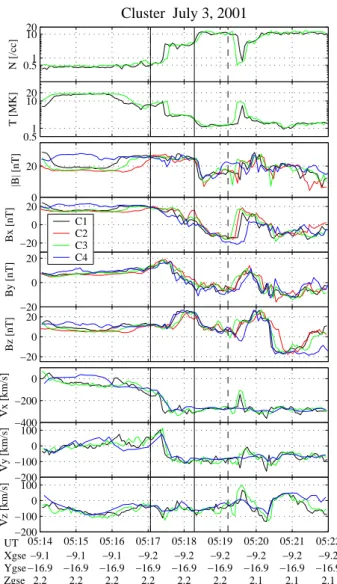
Figure 1 shows an overview of the data from the CIS (R`eme et al., 2001) and FGM (Balogh et al., 2001) instru-ments for an 8 min interval surrounding the event. From top to bottom, the panels show ion density, ion temperature, in-tensity and three GSE components of the magnetic field, and three GSE components of the ion flow velocity, respectively. The velocity values are from the HIA part of CIS for C1 and C3, whereas they are from the CODIF part for C4. The den-sity increased and the temperature decreased from their mag-netospheric to their magnetosheath values with two step-like changes, first, coincident with a rapid change in the veloc-ity, at ∼05:17:30 UT, and second at ∼05:18:20 UT. On the

(4)

H. Hasegawa et al.: Optimal magnetopause reconstruction from Cluster 975

other hand, the magnetic field varied more gradually, so that sufficient data points are available within the current layer. Because of the two-step behavior, the actual center times of the four magnetopause crossings cannot be unambiguously established. We use interval 1, between the two solid vertical lines, for the description of the methodology. In this inter-val, the field rotates with approximately constant magnitude. It is followed by an abrupt decrease in field magnitude that coincides with the second density/temperature step. The ex-tended interval 2, between the first solid line and the dashed line, which incorporates this decrease, is discussed in the last paragraph of Sect. 3.

2.2 Procedure

The reconstruction of an optimal magnetic field map by in-gestion of data from all four Cluster spacecraft proceeds as follows; a condensed version of the procedure, along with application to a flux transfer event, has been given by Son-nerup et al. (2004):

1. Determination of a common HT velocity is made by combining the velocity and magnetic field measure-ments during the analyzed interval from both C1 and C3, for which high time resolution velocity values are available (the CODIF measurements from C4 have lower time resolution). This, at the same time, allows a test of whether a good HT frame is found and for whether inertia effects can be neglected. In the case un-der discussion, the correlation coefficient between the GSE components of VH T×B and the corresponding components of V ×B is 0.983, and the Wal´en slope (the slope of regression in the scatter plot of the ve-locity components, transformed into the HT frame, ver-sus the corresponding components of the measured lo-cal Alfv´en velocity) is 0.318, satisfying both the above mentioned event selection criteria in Sect. 2.1, and thus confirming the suitability of the event for reconstruc-tion. The calculated HT frame velocity is (−327.9,

−99.2, −129.2) km in GSE. A constant HT veloc-ity is used for a first trial, but time-dependent HT velocity, which, for example, can be determined by sliding-window HT analysis (Hu and Sonnerup, 2003; Hasegawa et al., 2004), may sometimes be used, as for the event discussed in section 4.

2. The plasma pressure value, which is needed for calcu-lating the right-hand side of the GS equation, is esti-mated for all four spacecraft. We assume that only ions, assumed to be protons with isotropic temperature, con-tribute to the pressure. The pressure is then measured directly by CIS/HIA for C1 and C3. On the other hand, the pressure at C2 and C4 is deduced via electron den-sity measurements from the EFW instrument (Gustafs-son et al., 2001), which is operative on all four space-craft, in the following way. Rough values of the elec-tron density can be estimated from the spacecraft po-tential measurements by EFW (Pedersen et al., 2001).

0.51 10 20 N [/cc] Cluster July 3, 2001 0.51 10 20 T [MK] 0 20 |B| [nT] −20 0 20 Bx [nT] −20 0 20 By [nT] −20 0 20 Bz [nT] C1 C2 C3 C4 −400 −200 0 Vx [km/s] −200 −100 0 100 Vy [km/s] 05:14 05:15 05:16 05:17 05:18 05:19 05:20 05:21 05:22 −200 −100 0 100 Vz [km/s] UT Xgse Ygse Zgse −9.1 −16.9 2.2 −9.1 −16.9 2.2 −9.1 −16.9 2.2 −9.2 −16.9 2.2 −9.2 −16.9 2.2 −9.2 −16.9 2.2 −9.2 −16.9 2.1 −9.2 −16.9 2.1 −9.2 −16.9 2.1

Fig. 1. Time series of Cluster measurements around a magne-topause boundary layer traversal at ∼05:17:30 UT on 3 July 2001. The panels, from top to bottom, show ion number density, ion tem-perature, magnitude and three GSE components of the magnetic field, and three GSE components of the ion bulk velocity, respec-tively (black: spacecraft 1 (C1), red: C2, green: C3, blue: C4). The interval sandwiched between the two vertical solid lines (interval 1) is used for generating the map shown in Fig. 5, while the interval sandwiched between the first solid line and the dashed line (interval 2) is for the map in Fig. 7.

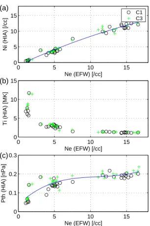
Figure 2 shows, from top to bottom, the relationship at C1 and C3 between ion density, ion temperature, and plasma pressure from CIS/HIA and the electron density from EFW, for the interval 05:17:04–05:19:13 UT. The estimated electron density is systematically larger than the ion density from CIS, as shown in the top panel. A polynomial function of the form p=p(Ne)is fitted to the data points in the bottom panel. We then use this function to estimate the pressure at C2 and C4 from the electron density values measured by them, the assump-tion being that the funcassump-tional relaassump-tionship, derived from

(5)

0 5 10 15 0 5 10 15 Ne (EFW) [/cc] Ni (HIA) [/cc] (a) C1 C3 0 5 10 15 0 5 10 15 Ne (EFW) [/cc] Ti (HIA) [MK] (b) 0 5 10 15 0 0.1 0.2 0.3 Ne (EFW) [/cc] Pth (HIA) [nPa] (c)

Fig. 2. Relationship from C1 and C3 between (a) ion density, (b), ion temperature, and (c) plasma pressure measured by the CIS/HIA instrument and electron density estimated from the spacecraft po-tential measurements by the EFW instrument.

the C1 and C3 data, holds at C2 and C4 as well. The underlying assumption of this procedure is that the ion temperature is constant in regions where the electron density has an equal value. In the event under discus-sion, this assumption appears to be reasonable on the scale of the spacecraft separation (∼2000 km), since the ion temperature from C1 and C3 is nearly the same at a certain electron density value (Fig. 2b).

3. Choice of a trial invariant z axis is made, leading to the establishment of a common reconstruction coordinate system. The partial vector potential A is then calculated from Eq. (2) and relationships between Pt and A, and between Bz and A are obtained along each of the four spacecraft trajectories. For each spacecraft, the value of A contains an arbitrary constant. This freedom is used to adjust the value of A at the start of the interval, for three of the spacecraft (C2, C3, and C4) in such a way that Pt and Bz from the four spacecraft agree as close as possible at each A value. These adjustments are equivalent to gauge transformations and are neces-sary because, in a magnetohydrostatic equilibrium, Pt and Bz should be constant along a field line, i.e. at a certain A value. The resulting relationships between Pt

−0.11 −0.05 0 0.05 0.1 0.15 2 3 4 5 6x 10 −10 A [T⋅m] P t = (p + B z 2 /2 µ 0 ) [Pa] July 3, 2001 051704−051817 UT −0.1 −0.05 0 0.05 0.1 0.15 −2.5 −2 −1.5 −1 x 10−8 A [T⋅m] B z [T]

Fig. 3. Transverse pressure Pt=(p + Bz2/2µ0)(top) and axial

mag-netic field component Bz (bottom) versus partial magnetic vector

potential A during the interval 1 of the 3 July 2001 event. The fitted curve is a polynomial function of A and is determined using the data points from all four spacecraft. Extrapolations at small and large A values are the straight-line segments.

and A and between Bzand A are shown in Fig. 3. The functions Pt(A)and Bz(A), which are now common to all four spacecraft, are determined from these plots by optimal fitting of a polynomial to the data points from all four spacecraft. That these fits are less than perfect is an indication of local deviations from the model as-sumptions. These deviations appear to have only a weak influence on the overall map configurations.

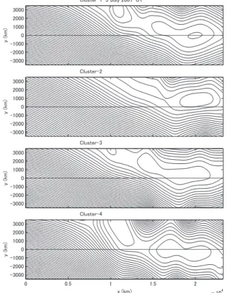
4. Four magnetic field maps are produced, one for each spacecraft. In each reconstruction, the integration of the GS equation is performed using the magnetic field measured along each spacecraft as the initial values, but using the common functions Pt(A)and Bz(A). The re-sulting four maps are shown in Fig. 4, in which black curves represent the transverse magnetic field lines and the x axis represents each spacecraft trajectory. With the exception that they are displaced relative to each other in the y direction, they are more or less similar, as they should be when the model assumptions are satisfied.

5. The four maps are merged into a single composite map, after weighting the A value at each grid point in each map with an appropriate function. In each map, nu-merical errors due to the integration develop; hence, the

(6)

H. Hasegawa et al.: Optimal magnetopause reconstruction from Cluster 977 䎐䎖䎓䎓䎓䎐䎕䎓䎓䎓䎐䎔䎓䎓䎓䎓䎔䎓䎓䎓䎕䎓䎓䎓䎖䎓䎓䎓䏜䎃䎋䏎䏐䎌䎦䏏䏘䏖䏗䏈䏕䎐䎔䎃䎃䎖䎃䎭䏘䏏䏜䎃䎕䎓䎓䎔䎃䎃䎸䎷䎐䎖䎓䎓䎓䎐䎕䎓䎓䎓䎐䎔䎓䎓䎓䎓䎔䎓䎓䎓䎕䎓䎓䎓䎖䎓䎓䎓䏜䎃䎋䏎䏐䎌䎦䏏䏘䏖䏗䏈䏕䎐䎖䎐䎖䎓䎓䎓䎐䎕䎓䎓䎓䎐䎔䎓䎓䎓䎓䎔䎓䎓䎓䎕䎓䎓䎓䎖䎓䎓䎓䏜䎃䎋䏎䏐䎌䎦䏏䏘䏖䏗䏈䏕䎐䎕䎓䎓䎑䎘䎔䎔䎑䎘䎕䏛䎃䎔䎓䎗䏛䎃䎋䏎䏐䎌䎐䎖䎓䎓䎓䎐䎕䎓䎓䎓䎐䎔䎓䎓䎓䎓䎔䎓䎓䎓䎕䎓䎓䎓䎖䎓䎓䎓䏜䎃䎋䏎䏐䎌䎦䏏䏘䏖䏗䏈䏕䎐䎗

Fig. 4. Magnetic field maps, each reconstructed for the interval 1 using the magnetic field measurements along each spacecraft tra-jectory as spatial initial values. Black contour lines represent the transverse (in-plane) magnetic field lines.

Avalues become less accurate as one moves in the ±y direction away from the spacecraft trajectory. This ef-fect is taken into account by use of a weight function. The A value at a chosen grid point of a common grid in the x−y plane is calculated by

Acomposit e(x, y) = 4 X i=1 Wi(y)Ai(x, y)/ 4 X i=1 Wi(y), (3)

where Aiis the value in the map from the i-th spacecraft at the chosen point. We use a Gaussian function as the weight,

Wi(y) =exp (−

1

2D2(y − yi)

2_), ₍₄₎

where yi is the y position of i-th spacecraft trajectory and D is the width of the Gaussian function. The top panel of Fig. 5 shows the composite field map thus ob-tained.

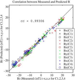
6. The correlation between the field components predicted from the composite map along the four spacecraft tra-jectories and the corresponding measured field compo-nents is shown in Fig. 6. We use this correlation as a measure of the quality of the map, since a good correla-tion means that each of the four individual maps predicts

0 0.5 1 1.5 2 x 104 −2000 −1000 0 1000 2000 20 nT N1 N2 N3 N4

Composite Map, 3 July 2001 051704−051817 UT

y [km] 1 2 3 4 [nT] Bz −30 −20 −10 0 0.5 1 1.5 2 x 104 −2000 −1000 0 1000 2000 y [km] 100 km/s 1 3 4 Pth [nPa] −V_HTx 0 0.1 0.2 0 0.5 1 1.5 2 x 104 −2000 −1000 0 1000 2000 x [km] y [km] Ni [/cc] 0 2 4

Fig. 5. Composite maps produced for the interval 1 by superposing and averaging the four field maps shown in Fig. 4 (see text for de-tails). In the reconstruction plane, the spacecraft move from left to

right: the magnetosphere where Bx>0; By<0 is on the lower left

side and the magnetosheath (Bx<0; By>0) is on the upper right

side. Color-coded in the panels are the magnetic field component normal to the plane, plasma pressure, and ion density, respectively. In the top panel, white arrows anchored at points along the space-craft trajectories represent the measured magnetic field vectors; yel-low arrows show the boundary normals, N 1−N 4, determined for

each spacecraft by MVAB with constraint hBni=0; line segments in

the upper part are GSE unit vectors, X (red), Y (green), and Z (yel-low), projected onto the x−y plane. In the middle panel, the white arrows represent the ion bulk velocity vectors from CIS/HIA (C1 and C3) or from CIS/CODIF (C4), transformed into the HT frame. GSE coordinate axes of the map are x=(0.9483, 0.2867, −0.1359),

y=(0.2895, −0.9572, 0.0006), z=(−0.1300, −0.0399, −0.9907).

well the field variations along the three spacecraft that are not used for each reconstruction and that the merg-ing of the four maps works successfully. The correlation coefficient, cc=0.9931, has been maximized by varying the choice of the invariant axis, the extrapolated por-tions of the funcpor-tions Pt(A)and Bz(A), and the width of the Gaussian weight function. This optimization is achieved only after a large number of reconstructions with different parameters has been performed. The op-timal invariant axis can be searched for in the way de-scribed by Hasegawa et al. (2004). The base coordinate system, in which a trial invariant axis is chosen, is deter-mined from minimum variance analysis using the com-bined magnetic field data (MVAB) (e.g. Sonnerup and Scheible, 1998) from all four spacecraft, with constraint

hBi·n =0, where n is the minimum variance direction.

As an experiment, a triangular rather than a Gaus-sian weight function has also been used, but the op-timal correlation coefficient is then lower than for the Gaussian function. In general, the correlation coeffi-cient becomes higher for a narrower width of the Gaus-sian function but too narrow weights result in unreal-istic discontinuous features in the composite field map. Thus, a not-too-narrow Gaussian function is chosen: the

(7)

−30 −20 −10 0 10 20 30 −30 −20 −10 0 10 20 30

Bi (Predicted) [nT] i=x,y,z for C1,2,3,4

Bi (Measured) [nT] i=x,y,z for C1,2,3,4 Correlation between Measured and Predicted B

cc = 0.99306 Bx(C1) By(C1) Bz(C1) Bx(C2) By(C2) Bz(C2) Bx(C3) By(C3) Bz(C3) Bx(C4) By(C4) Bz(C4)

Fig. 6. Scatter plot of three components of the measured versus the predicted magnetic field in the reconstruction coordinates.

width used for the map in Fig. 5 is 25% of the total width, in the y direction of the reconstruction domain. An optimal way to determine the width of the weight function has not yet been established; it is an issue for future study.

The composite map no longer satisfies the GS equation precisely. It accommodates, to some extent, deviations from the ideal model assumptions, such as inertia ef-fects, while preserving ∂/∂z=0 and time-independence. In Fig. 5, however, the deviation from the GS equa-tion turned out to be fairly small: an error measured as the local magnitude of ∇p−j×B normalized by that of j×B is 0.01 or less in most parts of the reconstruc-tion domain. A substantial deviareconstruc-tion is present along the boundary between the domain reconstructed based on the measurements and the domain based on the ex-trapolation in the vicinity of a major magnetic island at (x, y)∼(20 000, 0) km, because connection between the extrapolated curve and the fitted curve in Fig. 2 is not exactly smooth. A better extrapolation is an is-sue of future improvement. Once the optimum has been found, one can also produce maps exhibiting the plasma pressure, p, number density, N , and tempera-ture, T , by determining optimal functions p(A), N (A), and T (A). The axial current density, jz, is given by

jz(A)=dPt(A)/dA. The current density in the

recon-struction plane, jt, is parallel to the transverse field lines and is given by jt=(1/µ0)(dBz/dA)Bt, where Bt=(Bx, By). It is seen that the structures encountered are completely described in the MHD model.

3 Discussion of event on 3 July 2001, 05:17:30 UT The optimal field map for this event is shown in the top panel of Fig. 5, where field lines in the x−y plane are shown by black curves and the colors represent the axial (z) field com-ponent. The magnetosphere is on the lower left side and the magnetosheath is on the upper right side (the follow-ing maps always show the magnetosheath on the top and the magnetosphere on the bottom). White arrows anchored at points along the four spacecraft trajectories represent actu-ally measured magnetic field vectors projected onto the x−y plane. They are not exactly aligned with the reconstructed field lines for any of the four spacecraft because the map is a superposed version of the four individual maps (each of which shows exact agreement for the spacecraft data from which it is constructed). But the correlation coefficient be-tween the three components of the measured magnetic field and the corresponding components predicted from the map is very high (cc=0.9931), as shown in Fig. 6, which validates the procedure and indicates excellent accuracy of the com-posite map. For comparison, the correlation coefficients for the individual maps in Fig. 4 are, from top to bottom, 0.9852, 0.9802, 0.9827, and 0.9859, self-correlations excluded as in Hasegawa et al. (2004).

The current layer in the map has the thickness of more than 3000 km, which is much larger than the typical thick-nesses of the magnetopause current layer reported in the lit-erature (Berchem and Russell, 1982; Phan and Paschmann, 1996; Haaland et al., 2004), although it is not clear whether or not the current layer constitutes the true magnetopause (as discussed in Sect. 6). Prominent magnetic flux ropes are em-bedded in the current layer, indicating that magnetic recon-nection occurred to form them somewhere upstream of the spacecraft. Yellow arrows show the normal vectors deter-mined from MVAB with the constraint hBi·n =0 (MVABC) for each spacecraft. They are consistent with the map and suggest the presence of a systematically curved surface of the current layer.

The middle panel of Fig. 5 shows the same field lines but the colors now represent the thermal pressure and the white vectors show transverse velocities, Vt=(V −VH T)t, seen in the HT frame. These arrows are largest in the magneto-sphere. They are much smaller in the current layer, indicat-ing that the HT frame is well anchored to the plasma in the current layer and that there are no signatures of reconnection jets. The latter result is consistent with the high correlation coefficient. It indicates that the structures have reached an approximate equilibrium.

In the bottom panel of Fig. 5, the ion density is color-coded, assuming that the temperature and hence also the den-sity are constant along field lines. An important feature of this crossing is the presence of a substantial plasma bound-ary layer, immediately earthward of the current layer. The thickness of this boundary layer, defined by N >1 cc, is more than 3000 km. The result indicates that entry of the magne-tosheath plasma must have occurred to form the boundary

(8)

layer but does not help to identify the location or mechanism of the entry.

The optimal invariant axis, z, has GSE components (−0.1300, −0.0399, −0.9907). The angles, θ and φ, which define the z axis relative to the intermediate variance coordi-nate system, are 32◦and 4◦, respectively (see Hasegawa et al. (2004) for definition of these angles: θ =0, φ = 0 indicates the intermediate variance direction from MVABC and θ =−90,

φ=0 is the maximum variance direction). The magnetopause normal from MVABC, applied to the magnetic data from all four spacecraft, is (0.6901, −0.7110, −0.1352) in GSE. The result indicates that the invariant axis is more than 30 deg off the intermediate variance direction. It is approximately orthogonal to the normal, as expected, consistent with the finding by Hasegawa et al. (2004).

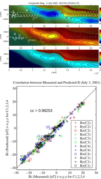
The improved technique is now applied to an extended interval (05:17:04−05:19:13 UT) of the event (interval 2 in Fig. 1). We here use the same invariant axis as in Fig. 5 while the HT frame velocity (VH T=(−300.9, −85.7, −92.9) km in GSE) and the functions Pt(A)and Bz(A)are determined in-dependently for this extended interval. The resulting com-posite maps and the corresponding scatter plot of predicted versus measured field components are shown in Fig. 7. The correlation coefficient of 0.9825 confirms that the map re-mains reasonably accurate. There is a prominent X point at

(x, y)∼(24 000, −1000) km. A substantial change in the

in-tensity of the axial field component occurs across the outer separatrix, a surface defined by field lines with their ends connected to the X point, on the magnetosheath side. This result indicates that another current layer, across which the field magnitude decreases rapidly, is present at the outer part of the whole magnetopause transition layer. The density map shows that the inner edge of the plasma boundary layer is not connected to the X point, but is located well inside the in-ner reconnection separatrix, i.e. on the magnetospheric side. (Note that concluding this is made possible thanks to the technique.) Thus, it cannot have been formed through re-connection at the X point in the map. Instead, the inner edge might be connected to a remote X line that is not seen in the map. Because of the abrupt changes in density, tempera-ture, and velocity at its inner edge, it seems unlikely that the boundary layer was produced by diffusive processes (see the Discussion Section).

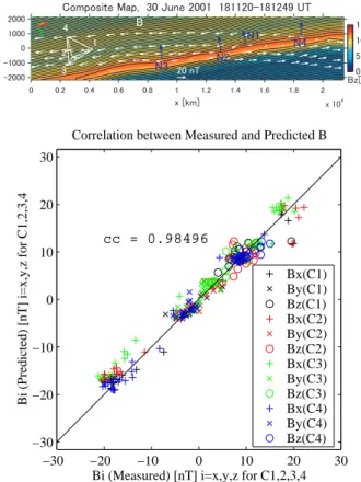
4 Cluster event on 30 June 2001, 18:12 UT

For further validation, the above improved method is now ap-plied to the magnetopause event on 30 June 2001 (18:12 UT), which has already been studied by use of the single-spacecraft based reconstruction method (Hasegawa et al., 2004). For this event, the pressure at C4 could not be esti-mated via the EFW measurements, since the potential of the satellite was controlled by the ASPOC instrument (Torkar et al., 2001). Therefore, the function Pt(A)is determined utilizing measurements from the other three spacecraft (C1, C2, and C3). Since the encountered magnetopause was under

0 0.5 1 1.5 2 2.5 3 3.5 x 104 −2000 0 2000 20 nT N1 N2 N3 N4 B

y [km] 1 2 3 4 [nT] Bz −30 −20 −10 0 0 0.5 1 1.5 2 2.5 3 3.5 x 104 −2000 0 2000 100 km/s x [km] y [km] 1 3 4 Pth [nPa] −V_HTx 0 0.1 0.2 0 0.5 1 1.5 2 2.5 3 3.5 x 104 −2000 0 2000 x [km] y [km] Ni [/cc] 0 5 10 −30 −20 −10 0 10 20 30 −30 −20 −10 0 10 20 30

Bi (Measured) [nT] i=x,y,z for C1,2,3,4

Correlation between Measured and Predicted B (July 3, 2001)

Fig. 7. Composite field maps and scatter plot of predicted versus measured field components for the interval 2 (the extended inter-val) of the 3 July 2001 event. In the top panel, white arrows show the measured field vectors and the colors represent the axial field component, while in the middle panel, the white arrows show the measured velocity vectors, seen in the HT frame, and the colors represent the plasma pressure. The bottom panel shows the ion den-sity color-coded. GSE coordinate axes of the map are x=(0.9532, 0.2702, −0.1359), y=(0.2732, −0.9620, 0.0029), with the same z axis as in Fig. 5.

significant acceleration (Hasegawa et al., 2004), we use time-dependent HT velocities, determined by sliding-window HT analysis, using the C1 and C3 data for determining the space-craft trajectories. Figure 8 shows a composite magnetic field map, along with the corresponding scatter plot. The invariant axis is found to be z=(0.5418, −0.0687, −0.8377) in GSE, which slightly deviates from the ones selected separately for C1 and C3 (Hasegawa et al., 2004). The deviations from the C1 and C3 invariant axes are 4.7◦and 6.4◦, respectively. The scatter plot shows the correlation coefficient of 0.9850, i.e. an improvement over the values of 0.9791 and 0.9799 found for the separate C1 and C3 reconstructions. The structures

(9)

䎓䎃䎘䎃䎔䎓䎔䎘䎓䎓䎑䎕䎓䎑䎗䎓䎑䎙䎓䎑䎛䎔䎔䎑䎕䎔䎑䎗䎔䎑䎙䎔䎑䎛䎕䏛䎃䎔䎓䎗䎐䎕䎓䎓䎓䎐䎔䎓䎓䎓䎓䎔䎓䎓䎓䎕䎓䎓䎓䎕䎓䎃䏑䎷䎱䎔䎱䎕䎱䎖䎱䎗䎥䎦䏒䏐䏓䏒䏖䏌䏗䏈䎃䎰䏄䏓䎏䎃䎃䎖䎓䎃䎭䏘䏑䏈䎃䎕䎓䎓䎔䎃䎃䎔䎛䎔䎔䎕䎓䎐䎔䎛䎔䎕䎗䎜䎃䎸䎷䏛䎃䎾䏎䏐䏀䏜䎃䎾䏎䏐䏀䎔䎕䎖䎗䎾䏑䎷䏀䎥䏝 −30 −20 −10 0 10 20 30 −30 −20 −10 0 10 20 30

Bi (Measured) [nT] i=x,y,z for C1,2,3,4 Correlation between Measured and Predicted B

Fig. 8. Composite map and associated scatter plot for a magne-topause crossing on 30 June 2001, to which the single spacecraft-based GS reconstruction method has been applied in earlier work (Hasegawa et al., 2004). The spacecraft trajectories for this event are determined by sliding-window HT analysis, based on the data from C1 and C3, from which high time resolution measurements are available for both velocity and magnetic field. GSE coordinate axes of the map are x=(0.7857, 0.3953, 0.4757), y=(0.2985, −0.9160, 0.2682), z=(0.5418, −0.0687, −0.8377).

are similar in the composite and the separate C1 and C3 maps, but some differences are found. In the composite map, the magnetopause surface is nearly flat, the thickness of the current layer is slightly larger, and there are no outstanding meso-scale structures within the current sheet. These differ-ences are the result of merging the four maps. The composite map suggests that the magnetopause observed was a tangen-tial discontinuity (TD), consistent with the Wal´en slope of 0.3452, based on the combined C1 and C3 data.

5 Cluster event on 5 July 2001, 06:23 UT

Hasegawa et al. (2004) found that, in the magnetopause event on 5 July 2001 (06:23 UT), there was significant temporal evolution of the current sheet structure in the interval be-tween the closely spaced traversals by C4 and C1 on the one hand, and the subsequent traversals by C2 and C3, on the other hand. For this reason, we produce two composite maps, one from C4 and C1, the other from C2 and C3. We use the HT velocity derived from C1 data for the first map and that

0 0.5 1 1.5 2 x 104 −2000 −1000 0 1000 2000 100 km/s N1 N2 N3 N4

x [km] y [km] 1 2 3 4 [nT] Bz 15 20 25 30 −40 −20 0 20 40 −40 −30 −20 −10 0 10 20 30 40

Fig. 9. Composite map produced from C1 and C4 measurements, and associated scatter plot for a magnetopause crossing on 5 July 2001, studied by Hasegawa et al. (2004). White arrows now repre-sent the velocity vectors transformed into the HT frame. GSE coor-dinate axes of the map are x=(0.7769, 0.2793, 0.5643), y=(0.3692,

−0.9280, −0.0490), z=(0.5100, 0.2464, −0.8241).

from C3 data for the second one, these velocity values are the same as used by Hasegawa et al. (2004). The resulting maps are shown in Figs. 9 and 10, respectively, along with the cor-responding scatter plots. The white arrows now represent ion bulk velocities, measured by CIS/HIA on board C1 and C3 and by CIS/CODIF on board C4, and transformed into the HT frame. Figure 9, produced from C4 and C1, shows that, at this time, the boundary was more or less of a TD-type, although two thin magnetic islands are present, separated by an X point at (x, y)=(10 000, 1000) km. In the HT frame, the velocities are small in the magnetosheath and much larger in the magnetosphere. This implies that the HT frame was well anchored in the magnetosheath plasma and that mag-netic coupling between the two sides was not strong. How-ever, the slope of the Wal´en regression line from C1 is +0.568 (Hasegawa et al., 2004), suggesting incipient reconnection at the X. The velocity arrows are not always well aligned with the field lines, in particular in the magnetosphere. The expla-nation for these deviations may lie in part in the intrinsic time dependence of the configuration and in part in the accuracy of the measurements.

The optimal invariant axis has GSE components

(10)

invariant axis selected for the separate C1 map (Hasegawa et al., 2004) by 8.3◦_{. The correlation coefficient of 0.9885,} shown in the scatter plot, is higher than the value for the C1-based map (0.9705), again indicating an improvement of the map.

Figure 10 shows the combined map generated from the C2 and C3 data. This map is dramatically different from the preceding one, indicating that there was significant tempo-ral evolution of the structure. A prominent magnetic island and field lines connecting the two sides of the magnetopause are now present. The velocities on the magnetosheath side, seen by C1, C3, and C4 in the HT frame, are now significant and are oriented mainly parallel to the magnetic field. The velocity vectors seen by C3 show a clear flow reversal near the island, consistent with the j ×B force acting on plasma flowing along the reconnected field lines. Field lines point-ing toward the magnetosphere, as well as the Wal´en slope (+1.03) from the C3 data, indicate that the magnetosheath plasma crosses the magnetopause and flows at the Alfv´en speed. These features are expected at a rotational discontinu-ity magnetopause that results from reconnection. In princi-ple, inertia forces associated with flow acceleration and time variation, both seen in the event, are not precisely dealt with by the GS reconstruction. The high correlation coefficient of 0.9883, however, verifies the qualitative accuracy of the map. Comparison of the two field maps in Figs. 9 and 10 enables us to identify the presence of significant local reconnection activity in the magnetopause, and to examine how the mag-netic field configuration changes in response to such local reconnection. Interestingly, the deviation (not shown) from the GS equation in the two maps is found to be larger than that in Fig. 5, consistent with the reconnection signatures. The optimal invariant axis is z=(0.6987, 0.3759, −0.6087) in GSE, which is almost the same as for the C3-based map (Hasegawa et al., 2004).

6 Summary and discussion

The primary results obtained in this study are as follows:

1. The GS reconstruction technique has been developed into a true multi-spacecraft method that produces a sin-gle magnetic field map using data from all four space-craft. An optimal field map can be generated by merg-ing four field maps, each of which is reconstructed usmerg-ing magnetic field measurements from one of the four Clus-ter spacecraft as spatial initial values but using common functions Pt(A)and Bz(A). The function Pt(A)can be determined on the basis of all four spacecraft measure-ments, by constructing a proxy for the pressure via elec-tron density measurements from EFW. The composite map leads to a substantially better agreement between the measured and predicted magnetic field values than can be achieved from the single-spacecraft based maps.

2. A higher correlation coefficient between the measured and predicted field components can be reached when a

䎓䎃䎔䎓䎕䎓䎖䎓䎗䎓䎓䎕䎓䎓䎓䎗䎓䎓䎓䎙䎓䎓䎓䎛䎓䎓䎓䎔䎓䎓䎓䎓䎔䎕䎓䎓䎓䎐䎕䎓䎓䎓䎐䎔䎓䎓䎓䎓䎔䎓䎓䎓䎕䎓䎓䎓䎔䎓䎓䎃䏎䏐䎒䏖䎱䎔䎱䎕䎱䎖䎱䎗䎦䏒䏐䏓䏒䏖䏌䏗䏈䎃䎰䏄䏓䎏䎃䎃䎘䎃䎭䏘䏏䏜䎃䎕䎓䎓䎔䎃䎃䎓䎙䎕䎕䎓䎓䎐䎓䎙䎕䎘䎕䎔䎃䎸䎷䏛䎃䎾䏎䏐䏀䏜䎃䎾䏎䏐䏀䎔䎕䎖䎗䎥䏝䎃䎾䏑䎷䏀 −40 −20 0 20 40 −40 −30 −20 −10 0 10 20 30 40

Fig. 10. Composite map produced from C2 and C3 measurements, and associated scatter plot for the 5 July 2001 event. GSE coordi-nate axes of the map are x=(0.6951, −0.1554, 0.7019), y=(0.1692,

−0.9135, −0.3699), z=(0.6987, 0.3759, −0.6087).

Gaussian-type rather than a triangular weight function of y is used for merging the four individual maps. Our experiment shows that a higher correlation is obtained for the Gaussian function with a width comparable to the spacecraft separation in the y direction, but an opti-mal way to determine the width has not yet been estab-lished.

3. An unusually thick (>3000 km) current sheet was found in the magnetopause transition layer on 3 July 2001 (05:18 UT). Also, prominent magnetic islands were em-bedded in the current sheet, demonstrating that the mag-netopause has substantial 2-D (and likely also 3-D) in-ternal magnetic structures. Reconnection that produced the islands must have occurred sufficiently much ear-lier than the encounter of the islands by Cluster, so that the observed structures had reached an approximate magnetohydrostatic equilibrium at the time of obser-vation. Two major current sheets were present in the whole magnetopause layer. These findings may shed new lights on the fundamental questions of what the magnetopause is and how it is formed.

(11)

4. A plasma boundary layer with a thickness of >3000 km was present immediately inside the magnetopause cur-rent layer on 3 July 2001 (05:18 UT), indicative of entry of the magnetosheath plasma across the boundary. In the map shown in Fig. 7, the inner edge of the bound-ary layer is not in the vicinity of the separatrix on the magnetospheric side. Note also that there is no discon-tinuous feature in the density map near the separatrix and that the inner edge appears to have a fairly sharp density and velocity gradient. These facts indicate that the observed boundary layer resulted from reconnec-tion, not from diffusive transport, and that the inner edge is connected to another X point that is not seen in, but exists outside of, the reconstruction domain shown in Fig. 7. Ion velocity distributions observed in the vicinity of the inner edge show the presence of two-component, magnetosheath-like ion populations, one streaming par-allel and the other streaming anti-parpar-allel to the field lines, although they do not have clear cutoffs, i.e. they are not D-shaped. Nevertheless, the distributions seem consistent with the view that the two populations are the result of remote reconnection.

5. In the 5 July 2001 event, there was significant time evolution of the structure associated with reconnection developing locally in the magnetopause current layer. Interestingly, the maps show that the axial magnetic field component was substantially larger in the mag-netosphere than in the magnetosheath, indicating that the orientation of the observed X line was closer to the magnetospheric field direction. This result leads to the following question: How does Nature determine the ori-entation of X lines in the presence of a guide field? This question is poorly understood, both theoretically and observationally (see, however, Swisdak et al., 2003). Examination of more events may provide insights into this issue.

Acknowledgements. We thank M. Andr´e and A. Vaivads for

provid-ing electron density data from the EFW instrument, L. Kistler and C. Mouikis for corrected CIS/CODIF data from C4, and T. Phan for plots of ion distributions. H. Hasegawa thanks A. Vaivads for his helpful comments on the manuscript. Research at Dartmouth Col-lege was supported by NASA grant NAG5-12005.

Topical Editor T. Pulkkinen thanks T. Carozzi and another ref-eree for their help in evaluating this paper.

References

Balogh, A., Carr, C. M., Acu˜na, M. H., et al.: The Cluster’ magnetic field investigation: overview of in-flight performance and initial results, Ann. Geophys., 19, 1207–1217, 2001,

SRef-ID: 1432-0576/ag/2001-19-1207.

Berchem, J. and Russell, C. T.: The thickness of the magnetopause current layer – ISEE 1 and 2 observations, J. Geophys. Res., 87, 2108–2114, 1982.

Gustafsson, G., Andre, M., Carozzi, T., et al.: First results of elec-tric field and density observations by Cluster EFW based on ini-tial months of operation, Ann. Geophys., 19, 1219–1240, 2001, SRef-ID: 1432-0576/ag/2001-19-1219.

Haaland, S. E., Sonnerup, B. U. ¨O., Dunlop, M. W., et al.:

Four-spacecraft determination of magnetopause orientation, motion and thickness: comparison with results from single-spacecraft methods, Ann. Geophys., 22, 1347–1365, 2004,

SRef-ID: 1432-0576/ag/2004-22-1347.

Hasegawa, H., Sonnerup, B. U. ¨O., Dunlop, M. W., Balogh, A.,

Haaland, S. E., Klecker, B., Paschmann, G., Lavraud, B., Dan-douras, I., and R`eme, H.: Reconstruction of two-dimensional magnetopause structures from Cluster observations: Verification of method, Ann. Geophys., 22, 1251–1266, 2004,

SRef-ID: 1432-0576/ag/2004-22-1251.

Hau, L.-N. and Sonnerup, B. U. ¨O.: Two-dimensional coherent

structures in the magnetopause: Recovery of static equilibria from single-spacecraft data, J. Geophys. Res., 104, 6899–6917, 1999.

Hu, Q. and Sonnerup, B. U. ¨O.: Magnetopause transects from two

spacecraft: A comparison, Geophys. Res. Lett., 27, 1443–1446, 2000.

Hu, Q. and Sonnerup, B. U. ¨O.: Reconstruction of magnetic flux

ropes in the solar wind, Geophys. Res. Lett., 28, 467–470, 2001.

Hu, Q. and Sonnerup, B. U. ¨O.: Reconstruction of magnetic clouds

in the solar wind: Orientation and configuration, J. Geophys. Res., 107(A7), 1142, doi:10.1029/2001JA000293, 2002.

Hu, Q. and Sonnerup, B. U. ¨O.: Reconstruction of two-dimensional

structures in the magnetopause: Method improvements, J. Geo-phys. Res., 108(A1), 1011, doi:10.1029/2002JA009323, 2003.

Khrabrov, A. V. and Sonnerup, B. U. ¨O.: DeHoffmann-Teller

anal-ysis, in: Analysis Methods for Multi-Spacecraft Data, ISSI Sci. Rep., SR-001, Kluwer Acad., Norwell, Mass., 221–248, 1998. Pedersen, A., Decreau, P., Escoubet, C.-P., Gustafsson, G., Laakso,

H., Lindqvist, P.-A., Lybekk, B., Masson, A., Mozer, F., and Vaivads, A.: Four-point high time resolution information on elec-tron densities by the electric field experiments (EFW) on Cluster, Ann. Geophys., 19, 1483–1489, 2001,

SRef-ID: 1432-0576/ag/2001-19-1483.

Phan, T.-D. and Paschmann, G.: Low-latitude dayside magne-topause and boundary layer for high magnetic shear 1. Structure and motion, J. Geophys. Res., 101, 7801–7815, 1996.

R`eme, H., Aoustin, C., Bosqued, J. M., et al.: First multispacecraft ion measurements in and near the Earth’s magnetosphere with the identical Cluster ion spectrometry (CIS) experiment, Ann. Geophys., 19, 1303–1354, 2001,

SRef-ID: 1432-0576/ag/2001-19-1303.

Sonnerup, B. U. ¨O. and Guo, M.,: Magnetopause transects,

Geo-phys. Res. Lett., 23, 3679–3682, 1996.

Sonnerup, B. U. ¨O. and Scheible, M.: Minimum and maximum

variance analysis, in: Analysis Methods for Multi-Spacecraft Data, ISSI Sci. Rep., SR-001, Kluwer Acad., Norwell, Mass., 185–220, 1998.

Sonnerup, B. U. ¨O., Hasegawa, H., and Paschmann, G.: Anatomy

of a flux transfer event seen by Cluster, Geophys. Res. Lett., 31, L11803, doi:10.1029/2004GL020134, 2004.

Swisdak, M., Rogers, B. N., Drake, J. F., and Shay, M. A.: Diamagnetic suppression of component magnetic reconnec-tion at the magnetopause, J. Geophys. Res., 108(A5), 1218, doi:10.1029/2002JA009726, 2003.

Torkar, K., Riedler, W., Escoubet, C. P., et al.: Active spacecraft potential control for Cluster – implementation and first results, Ann. Geophys., 19, 1289–1302, 2001,