Adaptive nonparametric estimation of a component density in a two-class mixture model

Adaptive nonparametric estimation of a component density in a

two-class mixture model

Ga¨

elle Chagny

_{, Antoine Channarond}

_{, Van H`}

_{a Hoang}

_{, Angelina Roche}

July 30, 2020

Abstract

A two-class mixture model, where the density of one of the components is known, is considered. We address the issue of the nonparametric adaptive estimation of the unknown probability density of the second component. We propose a randomly weighted kernel estimator with a fully data-driven bandwidth selection method, in the spirit of the Goldenshluger and Lepski method. An oracle-type inequality for the pointwise quadratic risk is derived as well as convergence rates over H¨older smoothness classes. The theoretical results are illustrated by numerical simulations.

1

Introduction

The following mixture model with two components:

g_{pxq “ θ ` p1 ´ θqfpxq, @x P r0, 1s,} (1)

where the mixing proportion θ P p0, 1q and the probability density function f on r0, 1s are unknown, is considered in this article. It is assumed that n independent and identically distributed (i.i.d. in the sequel) random variables X1, . . . , Xn drawn from density g are observed. The main goal is to construct

an adaptive estimator of the nonparametric component f and to provide non-asymptotic upper bounds of the pointwise risk. As an intermediate step, the estimation of the parametric component θ is addressed as well.

Model (1) appears in some statistical settings, robust estimation and multiple testing among oth-ers. The one chosen in the present article, as described above, comes from the multiple testing frame-work, where a large number n of independent hypotheses tests are performed simultaneously. p-values X1, . . . , Xn generated by these tests can be modeled by (1). Indeed these are uniformly distributed on

r0, 1s under null hypotheses while their distribution under alternative hypotheses, corresponding to f, is unknown. The unknown parameter θ is the asymptotic proportion of true null hypotheses. It can be needed to estimate f , especially to evaluate and control different types of expected errors of the testing procedure, which is a major issue in this context. See for instance Genovese and Wassermann [15], Storey [28], Langaas et al. [20], Robin et al. [26], Strimmer [29], Nguyen and Matias [23], and more fundamentally, Benjamini et al. [1] and Efron et al. [14].

In the setting of robust estimation, different from the multiple testing one, model (1) can be thought of as a contamination model, where the unknown distribution of interest f is contaminated by the uniform distribution onr0, 1s with the proportion θ. This is a very specific case of the Huber contamination model [18]. The statistical task considered consists in robustly estimating f from contaminated observations X1, . . . , Xn. But unlike our setting, the contamination distribution is not necessarily known while the

contamination proportion θ is assumed to be known and the theoretical investigations aim at providing minimax rates as functions of both n and θ. See for instance the preprint of Liu and Gao [22], which addresses pointwise estimation in this framework.

∗_{LMRS, UMR CNRS 6085, Universit´e de Rouen Normandie, gaelle.chagny@univ-rouen.fr} †_{LMRS, UMR CNRS 6085, Universit´e de Rouen Normandie, antoine.channarond@univ-rouen.fr} ‡_{LMRS, UMR CNRS 6085, Universit´e de Rouen Normandie, van-ha.hoang@univ-rouen.fr} §_{CEREMADE, UMR CNRS 7534, Universit´e Paris Dauphine, roche@ceremade.dauphine.fr}

Back to the setting of multiple testing, the estimation of f in model (1) has been addressed in several works. Langaas et al. [20] proposed a Grenander density estimator for f , based on a nonparametric maximum likelihood approach, under the assumption that f belongs to the set of decreasing densities on r0, 1s. Following a similar approach, Strimmer [29] also proposed a modified Grenander strategy to estimate f . However, the two aforementioned papers do not investigate theoretical features of the proposed estimators. Robin et al. [26] and Nguyen and Matias[23] proposed a randomly weighted kernel estimator of f , where the weights are estimators of the posterior probabilities of the mixture model, that is, the probabilities of each individual i being in the nonparametric component given the observation Xi.

[26] proposes an EM-like algorithm, and proves the convergence to an unique solution of the iterative procedure, but they do not provide any asymptotic property of the estimator. Note that their model g<sub>pxq “ θφpxq ` p1 ´ θqfpxq, where φ is a known density, is slightly more general, but our procedure is</sub> also suitable for this model under some assumptions on φ. Besides, [23] achieves a nonparametric rate of convergence n´2β{p2β`1q _{for their estimator, where β is the smoothness of the unknown density f .}

However, their estimation procedure is not adaptive since the choice of their optimal bandwidth still depends on β.

In the present work, a new randomly weighted kernel estimator is proposed. Unlike the usual approach in mixture models, the weights of the estimator are not estimates of the posterior probabilities. A function w is derived instead such that fpxq “ wpθ, gpxqqgpxq, for all θ, x P r0, 1s. This kind of equation, linking the target distribution (one of the conditional distribution given hidden variables) to the distribution of observed variables, is remarkable in the framework of mixture models. It is a key idea of our approach, since it implies a crucial equation for controlling the bias term of the risk, see Subsection 2.1 for more details. Thus oracle weights are defined by wpθ, gpXiqq, i “ 1, . . . , n, but g and θ are unknown. These

oracle weights are estimated by plug-in, using preliminary estimators of g and θ, based on an additional sample Xn`1, . . . , X2n. Note that procedures of [23] and [26] actually require preliminary estimates of g

and θ as well, but they do not deal with possible biases caused by the multiple use of the same observations in the estimates of θ, g and f .

Furthermore a data-driven bandwidth selection rule is also constructed in this paper, using the Gold-enshluger and Lespki (GL) approach [17], which has been applied in various contexts, see for instance, Comte et al. [11], Comte and Lacour [9], Doumic et al. [13], Reynaud-Bouret et al. [25] who apply GL method in kernel density estimation, and Bertin et al. [3], Chagny [6], Chichignoud et al. [7] or Comte and Rebafka [12]. Our selection rule is then adaptive to unknown smoothness of the target function, which is new in this context. The main original results derived in this paper are the oracle-type inequality in Theorem 1, and the rates of convergence over H¨older classes, which are adapted to the control of pointwise risk of kernel estimators, in Corollary1.

Some assumptions on the preliminary estimators for g and θ are needed to prove the results on the estimator of f ; this paper also provides estimators of g and θ which satisfy these assumptions. The choice of a nice estimator for θ requires identifiability of the model (1). g being given, the couplepθ, fq such that g _{“ θ ` p1 ´ θqf is uniquely determined under additional assumptions on f (in particular monotonicity} and zero set of f ), see a review about this issue in Section 1.1 in Nguyen and Matias [24]. Nonetheless, note that these additional assumptions on f are not needed to obtain the results on the nonparametric estimation procedure of f .

The paper is organized as follows. Our randomly weighted estimator of f is constructed in Section

2.1. Assumptions on f and on preliminary estimators of g and θ required for proving the theoretical results are in this section too. In Section 2, a bias-variance decomposition for the pointwise risk of the estimator of f is given as well as the convergence rate of the kernel estimator with a fixed bandwidth. In Section3, an oracle inequality which justifies our adaptive estimation procedure. Construction of the preliminary estimators of g and θ are to be found in Section4. Numerical results illustrate the theoretical results in Section 5. Proofs of theorems, propositions and technical lemmas are postponed to Section6.

2

Collection of kernel estimators for the target density

In this section, a family of kernel estimators for the density function f based on a sample pXiqi“1,...,n

of i.i.d. variables with distribution g is defined. It is assumed that two preliminary estimators ˜θn of

the mixing proportion θ and ˆg of the mixture density g are available, and defined from an additional sample pXiqi“n`1,...,2n of independent variables also drawn from g but independent of the first sample

pXiqi“1,...,n. The definition of these preliminary estimates is the subject of Section4.

2.1

Construction of the estimators

To define estimators for f , the challenge is that observations X1, . . . , Xn are not drawn from f but from

the mixture density g. Hence the density f cannot be estimated directly by a classical kernel density estimator. We will thus build weighted kernel estimates, using a methodology inspired for example by Comte and Rebafka [12]. The starting point is the following lemma whose proof is straightforward. Lemma 1. Let X be a random variable from the mixture density g defined by (1) and Y be an (unob-servable) random variable from the component density f . Then for any measurable bounded function ϕ we have E_{“ϕpY q‰ “ E“wpθ, gpXqqϕpXq‰, (2)} with wpθ, gpxqq :“ 1 1´ θ ˆ 1´ θ gpxq ˙ , xP r0, 1s.

This result will be used as follows. Let K : RÑ R be a kernel function, that is an integrable function such that ş

RKpxqdx “ 1 and

ş

RK

2_{pxqdx ă `8. For any h ą 0, let K}

hp¨q “ Kp¨{hq{h. Then the choice

ϕp¨q “ Khpx ´ ¨q in Lemma 1leads to

E“K_{hpx ´ Y1}q‰ “ E“wpθ, gpX_{1qqKhpx ´ X1q}‰, where Y is drawn from g. Thus,

ˆ fhpxq “ 1 n n ÿ i“1 wp˜θn,ˆgpXiqqKhpx ´ Xiq, x P r0, 1s, (3)

is well-suited to estimate f , with

w_p˜θn,ˆgpXiqq “ 1 1´ ˜θn ˜ 1´_ˆθ˜n gpXiq ¸ , i_{“ 1, . . . , n.}

Therefore, ˆfh is a randomly weighted kernel estimator of f . However, the total sum of the weights

may not equal 1, in comparison with the estimators proposed in Nguyen and Matias [23] and Robin et al. [26]. The main advantage of our estimate is that, if we replace ˆgand ˜θn by their theoretical unknown

counterparts g and θ in (3), we obtain, Er ˆfhpxqs “ Kh‹ fpxq, where ‹ stands for the convolution product.

This relation, classical in nonparametric kernel estimation, is crucial for the study of the bias term in the risk of the estimator.

2.2

Risk bounds of the estimator

Here, we establish upper bounds for the pointwise mean-squared error of the estimator ˆfh, defined in

(3), with a fixed bandwidth hą 0. Our objective is to study the pointwise risk for the estimation of the density f at a point x0P r0, 1s. Throughout the paper, the kernel K is chosen compactly supported on

an interval r´A, As with A a positive real number. We denote by Vnpx0q the neighbourhood of x0used

in the sequel and defined by

Vnpx0q “ „ x0´ 2A αn , x0` 2A αn  ,

where pαnqn is a positive sequence of numbers larger than 1, only depending on n such that αn Ñ `8

as nÑ `8. For any function u on R, and any interval I Ă R, let }u}8,I “ suptPI|uptq|.

The following assumptions will be required for our theoretical results.

(A2) The preliminary estimator ˆg is bounded away from 0 on Vnpx0q :

ˆ

γ :“ inf

tPVnpx0q

|ˆgptq| ą 0. (4)

(A3) The preliminary estimate ˆg of g satisfies, for all νą 0 P ˜ sup tPVnpx0q ˇ ˇ ˇ ˇ ˆ g_{ptq ´ gptq} ˆ gptq ˇ ˇ ˇ ˇą ν ¸ ď Cg,νexp ! ´plog nq3{2)_{, (5)}

with Cg,ν a constant only depending on g and ν.

(A4) The preliminary estimator ˜θn is constructed such that ˜θnP rδ{2, 1 ´ δ{2s, for a fixed δ P p0, 1q.

(A5) For any bandwidth hą 0, we assume that αnď 1 h and 1 hď ˆ γn log3pnq.

(A6) f belongs to the H¨older class of smoothness β and radius L on r0, 1s, defined by

Σpβ, Lq “!φ : φhas ℓ“ tβu derivatives and @x, y P r0, 1s, |φpℓqpxq ´ φpℓqpyq| ă L|x ´ y|β´ℓ), (A7) K is a kernel of order ℓ“ tβu : ş

Rx

j_{Kpxqdx “ 0 for 1 ď j ď ℓ and}ş

R|x|

ℓ_{|Kpxq|dx ă 8.}

Since g“ θ `p1´θqf, Assumption (A1) implies that }g}_8,Vnpx0qă 8. The latter condition is needed

to control the variance term, among others, of the bias-variance decomposition of the risk. Notice that the density g is automatically bounded from below by a positive constant in our model (1). Assumption (A2) is required to bound the term 1{ˆgp¨q that appears in the weight wp˜θn,ˆgp¨qq. Assumption (A3) means

that the preliminary ˆg has to be rather accurate. Assumptions(A2) and (A3) are also introduced by Bertin et al. [2] for conditional density estimation purpose : see (3.2) and (3.3) p.946. The methodology used in our proofs is inspired from their work : the role played by g here corresponds to the role plays by the marginal density of their paper. They have also shown that an estimator of g satisfying these properties can be built, see Theorem 4, p. 14 of [2] and some details at Section 4.1. We also build an estimator ˜θn that satisfied Assumption (A4) in Section 4.2. Assumption (A5) deals with the order of

magnitude of the bandwidths and is also borrowed from [2] (see Assumption (CK) p.947). Assumptions (A6) and (A7) are classical for kernel density estimation, see [30] or [10]. The index β in Assumption (A6) is a measure of the smoothness of the target function. It permits to control the bias term of the bias-variance decomposition of the risk, and thus to derive convergence rates.

We first state an upper bound for the pointwise risk of the estimator ˆfh. The proof can be found in

Section 6.1.

Proposition 1. Assume that Assumptions (A1) to (A5) are satisfied. Then, for any x0 P r0, 1s and

δP p0, 1q, the estimator ˆfh defined by (3) satisfies

E”`fˆhpx0q ´ fpx0q ˘2ı ď C1˚ " }Kh‹ f ´ f} 2 8,Vnpx0q` 1 δ2_γ2_nh * `C2˚ δ6E ”<sub>ˇ</sub> ˇ ˜θn´ θ ˇ ˇ 2ı ` C3˚ δ2_γ2E ” }ˆg ´ g}2_8,Vnpx0q ı ` C4˚ δ2_n2, (6) where C˚

ℓ, ℓ“ 1, . . . , 4 are positive constants such that : C1˚depends on}K}2and}g}_8,Vnpx0q, C ˚

2 depends

on }g}_8,Vnpx0q and}K}1, C ˚

3 depends on}K}1 and C4˚ depends on}f}_8,Vnpx0q, g and}K}8.

Proposition 1 is a bias-variance decomposition of the risk. The first term in the right-hand-side (r.h.s. in the sequel) of (6) is a bias term which decreases when the bandwidth h goes to 0 whereas the second one corresponds to the variance term and increases when h goes to 0. There are two additional terms Er}ˆg ´ g}2_8,Vnpx0qs and Er|ˆθn´ θ|

2_{s in the r.h.s. of (6). They are unavoidable since the estimator}

ˆ

fh depends on the plug-in estimators ˆg and ˜θn. The term C4˚{pδ2n2q is a remaining term and is also

negligible. However, the convergence rate that we derive in Corollary 1below will prove that these last three terms in (6) are negligible if g and θ are estimated accurately : Section4 proves that it is possible.

3

Adaptive pointwise estimation

Let Hn be a finite family of possible bandwidths hą 0, whose cardinality is bounded by the sample size

n. The best estimator in the collection p ˆfhqhPHn defined in (3) at the point x0 is the one that have the

smallest risk, or similarly, the smallest bias-variance decomposition. But since f is unknown, in practice it is impossible to minimize over Hnthe r.h.s. of inequality (6) in order to select the best estimate. Thus,

we propose a data-driven selection, with a rule in the spirit of Goldenshluger and Lepski (GL in the sequel) [17]. The idea is to mimic the bias-variance trade-off for the risk, with empirical counterparts for the unknown quantities. We first estimate the variance term of the trade-off by setting, for any hP Hn

V_px0, hq “ κ}K}21}K} 2 2}g}_8,Vnpx0q ˆ γ2_nh logpnq, (7)

with κ ą 0 a tuning parameter. The principle of the GL method is then to estimate the bias term }Kh‹ f ´ f}

2

8,Vnpx0qof ˆfhpx0q for any h P Hn with

Apx0, hq :“ max h1_PHn ! `ˆ fh,h1px<sub>0</sub>q ´ ˆf<sub>h</sub>1px<sub>0</sub>q˘ 2 ´ V px0, h1q ) `,

where, for any h, h1_{P H} n, ˆ fh,h1px₀q “ 1 n n ÿ i“1 w_p˜θn,gˆpXiqqpKh‹ Kh1qpx₀´ X_iq “ pK_h1‹ ˆf_hqpx₀q.

Heuristically, since ˆfh is an estimator of f then ˆfh,h1 “ K_h1 ‹ ˆf_h can be considered as an estimator of

Kh1‹ f. The proof of Theorem1below in Section6.4then justifies that Apx₀, hq is a good approximation

for the bias term of the pointwise risk. Finally, our estimate at the point x0is

ˆ

fpx0q :“ ˆfˆ_hpx0qpx0q, (8)

where the bandwidth ˆhpx0q minimizes the empirical bias-variance decomposition :

ˆ

h_px0q :“ argmin hPHn

Apx0, hq ` V px0, hq( .

The constants that appear in the estimated variance Vpx0, hq are known, except κ, which is a numerical

constant calibrated by simulation (see practical tuning in Section 5), and except }g}_8,Vnpx0q, which is

replaced by an empirical counterpart in practice (see also Section 5). It is also possible to justify the substitution from a theoretical point of view, but it adds cumbersome technicalities. Moreover, the replacement does not change the result of Theorem1below. We thus refer to Section 3.3 p.1178 in [8] for example, for the details of a similar substitution. The risk of this estimator is controlled in the following result.

Theorem 1. Assume that Assumptions (A1) to (A5) are fulfilled, and that the sample size n is larger than a constant that only depends on the kernel K. For any δP p0, 1q, the estimator ˆf_px0q defined in (8)

satisfies E”`<sub>ˆ</sub> fpx0q ´ fpx0q ˘2ı ď C˚ 5 min hPHn " }Kh‹ f ´ f}2<sub>8,Vnpx</sub>0q` logpnq δ2_γ2_nh * `C6˚ δ6 sup θPrδ,1´δs E”ˇˇ ˜θn´ θ ˇ ˇ 2ı ` C7˚ δ2_γ2E ” }ˆg ´ g}2_8,Vnpx0q ı ` C8˚ δ2_γ2_n2, (9) where C˚

ℓ, ℓ“ 5, . . . , 8 are positive constants such that : C5˚ depends on}g}_8,Vnpx0q,}K}1 and}K}2, C ˚ 6

depends on }K}1, C7˚ depends on }g}_8,Vnpx0q and }K}1, and C ˚

8 depends on }f}_8,Vnpx0q, g, }K}2 and

}K}₈.

Theorem 1 is an oracle-type inequality. It holds whatever the sample size, larger than a fixed con-stant. It shows that the optimal bias variance trade-off is automatically achieved: the selection rule

permits to select in a data-driven way the best estimator in the collection of estimators p ˆfhqhPHn, up

to a multiplicative constant C˚

6. The last three remainder terms in the r.h.s. of (9) are the same as

the ones in Proposition 1, and are unavoidable, as aforementioned. We have an additional logarithmic term in the second term of the r.h.s., compared to the analogous term in (6). It is classical in adaptive pointwise estimation (see for example [12] or [4]). In our framework, it does not deteriorate the adaptive convergence rate. The risk of the estimator ˆfpx0q with data-driven bandwidth decreases at the optimal

minimax rate of convergence (up to a logarithmic term) if the bandwidth is well-chosen : the upper bound of Corollary1 matches with the lower-bound for the minimax risk established by Ibragimov and Hasminskii [19].

Corollary 1. Assume that (A6) and (A7) are satisfied, for β ą 0 and L ą 0, and for an index ℓ ą 0 such that ℓě tβu. Suppose also that the assumptions of Theorem1are satisfied, and that the preliminary estimates ˜θn and ˆg are such that

E”_{|˜θn´ θ|}2ı_{ď C}ˆ log n n ˙ 2β 2β`1 , E”}ˆg ´ g}2<sub>8,V</sub>npx0q ı ď Cˆ log n n ˙ 2β 2β`1 . (10) Then, E”`fˆ<sub>px</sub>0q ´ fpx0q ˘2ı ď C9˚ ˆ log n n ˙ 2β 2β`1 , (11) where C˚

9 is a constant depending on}g}_8,Vnpx0q,}K}1,}K}2, L and}f}8,Vnpx0q.

The estimator ˆf now achieves the convergence rateplog n{nq2β{p2β`1q_{over the class Σpβ, Lq as soon as}

β ď ℓ. It automatically adapts to the unknown smoothness of the function to estimate : the bandwidth ˆ

hpx0q is computed in a fully data-driven way, without using the knowledge of the regularity index β,

contrary to the estimator ˆfnrwk of Nguyen and Matias [23] (corollary 3.4). Section 4 below permits to

also build ˆg and ˜θn without any knowledge of β, to obtain an automatic adaptive estimation procedure.

Remark 1. In the present work, we focus on Model (1). However, the estimation procedure we develop can easily be extended to the model

g_{pxq “ θφpxq ` p1 ´ θqfpxq,} x_{P R,} (12)

where the function φ is a known density, but not necessarily equal to the uniform one. In this case, a family of kernel estimates can be defined like in (3) replacing the weights wp˜θn,ˆgp¨qq by

w_p˜θn,gˆp¨q, φpx0qq “ 1 1´ ˜θn ˜ 1´θ˜n_ˆφpx0q gp¨q ¸ .

If the density function φ is uniformly bounded on R, it is then possible to obtain analogous results (bias-variance trade-off for the pointwise risk, adaptive bandwidth selection rule leading to oracle-type inequality and optimal convergence rate) as we established for model (1).

4

Estimation of the mixture density

g and the mixing

propor-tion

θ

This section is devoted to the construction of the preliminary estimators ˆg and ˜θn, required to build

(3). To define them, we assume that we observe an additional sample pXiqi“n`1,...,2n distributed with

density function g, but independent of the samplepXiqi“1,...,n. We explain how estimators ˆgand ˜θn can

be defined to satisfy the assumptions described at the beginning of Section2.2, and also how we compute them in practice. The reader should bear in mind that other constructions are possible, but our main objective is the adaptive estimation of the density f . Thus, further theoretical studies are beyond the scope of this paper.

4.1

Preliminary estimator for the mixture density

g

As already noticed, the role plays by g to estimate f in our framework finds an analogue in the work of Bertin et al. [3] : the authors propose a conditional density estimation method that involves a preliminary estimator of the marginal density of a couple of real random variables. The assumptions (A2) and (A3) are borrowed to their paper. From a theoretical point of view, we thus also draw inspiration from them to build ˆg.

Since we focus on kernel methods to recover f , we also use kernels for the estimation of g. Let L : R Ñ R be a function such thatş

RLpxqdx “ 1 and

ş

RL

2_{pxqdx ă 8. Let L}

bp¨q “ b´1Lp¨{bq, for any

hą 0. The function L is a kernel, but can be chosen differently from the kernel K used to estimate the density f . The classical kernel density estimate for g is

ˆ gbpx0q “ 1 n 2n ÿ i“n`1 Lbpx0´ Xiq, (13)

Theorem 4 p.14 of [2] proves that it is possible to select an adaptive bandwidth b of ˆgb in such a way that

Assumptions (A2) and (A3) are fulfilled, and that the resulting estimate ˆgˆ_b satisfies

E”›_›ˆgˆ b´ g › › 2 8,Vnpx0q ı ď Cˆ log n n ˙2β`12β ,

if gP Σpβ, L1_{q, where C, L}1_{ą 0 are some constants, and if the kernel L has an order ℓ “ tβu. The idea of}

the result of Theorem 4 in [2] is to select the bandwidth ˆb with a classical Lepski method, and to apply results from Gin´e and Nickl [16]. Notice that, in our model, Assumption (A6) permits to obtain directly the required smoothness assumption, gP Σpβ, L1_{q. This guarantees that both the assumptions (A2) and}

(A3) on ˆg can be satisfied and that the additional term Er}ˆg ´ g}2_8,Vnpx0qs can be bounded as required

in the statement of Corollary1.

For the simulation study below now, we start from the kernel estimatorspˆgbqbą0 defined in (13) and

rather use a procedure in the spirit of the pointwise GL method to automatically select a bandwidth b. First, this choice permits to be coherent with the selection method chosen for the main estimators p ˆfhqhPHn, see Section3. Then, the construction also provides an accurate estimate of g, see for example

[10]. Let B be a finite family of bandwidths. For any b, b1 _{P B, we introduce the auxiliary functions}

ˆ

gb,b1px₀q “ n´1ř2n

i“n`1pLb‹ Lb1qpx₀´ X_iq. Next, for any b P B, we set

Agpb, x0q “ max b1_PB ! `ˆgb,b1px<sub>0</sub>q ´ ˆg<sub>b</sub>1px<sub>0</sub>q˘ 2 ´ Γ1pb1q ) `, where Γ1pbq “ ǫ }L} 2 1}L} 2

2}g}₈logpnq{pnbq, with ǫ ą 0 a constant to be tuned. Then, the final estimator

of g is given by ˆgpx0q :“ ˆgˆ_b

gpx0qpx0q, with ˆbgpx0q :“ argminbPBtA g_{pb, x}

0q ` Γ1pbqu. The tuning of the

constant ǫ is presented in Section5.

4.2

Estimation of the mixing proportion

θ

A huge variety of methods have been investigated for the estimation of the mixing proportion θ of model (1) : see, for instance, [28], [20], [26], [5], [24] and references therein. A common and performant estimator is the one proposed by Storey [28]: θ is estimated by ˆθτ,n“ #tXią τ; i “ n ` 1, . . . , 2nu{pnp1 ´ τqq with

τ a threshold to be chosen. The optimal value of τ is calculated with a boostrap algorithm. However, it seems difficult to obtain theoretical guarantees on ˆθτ,n. To our knowledge, most of the other methods in

the literature rely on different identifiability constraints for the parameterspθ, fq. We refer to Celisse and Robin [5] or Nguyen and Matias [24] for a detailed discussion about possible identifiability conditions of model (1). In the sequel we focus on a particular case of model (1), that permits to obtain the identiability of the parameters pθ, fq (see for example Assumption A in [5], or Section 1.1 in [24]). The density f is assumed to belong to the family

F_{δ “ f : r0, 1s Ñ R`, f is a continuously non-increasing density, positive onr0, 1 ´ δq}

where δ P p0, 1q. Starting from this set, the main idea to recover θ is that it is the lower bound of the density g in model (1) : θ“ infxPr0,1sgpxq “ gp1q. Celisse and Robin [5] or Nguyen and Matias [24] then

define a histogram-based estimator ˆgfor g, and estimate θ with the lower bound of ˆg, or with ˆgp1q. The procedure we choose is in the spirit of this one, but, to be coherent with the other estimates, we use kernels to recover g instead of histograms.

Nevertheless, we cannot directly use the kernel estimates of g defined in (13): it is well-known that kernel density estimation methods suffers from boundary effects, which lead to an inaccuracy estimate of gp1q. To avoid this problem, we apply a simple reflection method inspired by Schuster [27]. From the random sample Xn`1, . . . , X2n from density g, we introduce, for k“ i ´ n, i “ n ` 1, . . . , 2n,

Yk “

#

Xi if ǫi“ 1,

2´ Xi if ǫi“ ´1,

where ǫn`1, . . . , ǫ2n are n i.i.d. random variables drawn from Rademacher distribution with parameter

1{2, and independent of the Xi’s. The random variables Y1, . . . , Yn can be regarded as symmetrized

version of the Xi’s, with supportr0, 2s (see the first point of Lemma2below). Now, suppose that L is a

symmetric kernel. For any bą 0, define ˆ gsym_b pxq “_2n1 n ÿ k“1 “Lbpx ´ Ykq ` Lbpp2 ´ xq ´ Ykq‰ , xP r0, 2s. (15)

The graph of ˆg_bsymis symmetric with respect to the straight-line x“ 1. Then, instead of evaluating ˆgsymb

at the single point x “ 1, we compute the average of all the values of the estimator ˆgb on the interval

r1 ´ δ, 1s, relying on the fact that θ “ gpxq, for all x P r1 ´ δ, 1s (under the assumption f P Fδ), to increase

the accuracy of the resulting estimate. Thus, we set ˆ θn,b“ 2 δ ż1 1_´δ ˆ g_bsym_pxqdx. (16)

Finally, for the estimation of f , we use a truncated estimator ˜θn defined as

˜

θn,b:“ max` minpˆθn,b,1´ δ{2q, δ{2˘. (17)

The definition of ˜θn,bpermits to ensure that ˜θn,bP rδ{2, 1 ´ δ{2s : this is Assumption (A4). This permits

to avoid possible difficulties in the estimation of f when ˆθn,bis close to zero, see (3). The following lemma

establishes some properties of all these estimates. Its proof can be found in Section6.2. Lemma 2.

• _{The estimator ˆg}sym

b defined in (15) has the same distribution as a classical kernel estimator from the

symmetrized density of g. More precisely, letpRiqiPt1,...,nu be i.i.d. random variables with density

r : x ÞÝÑ "

gpxq{2 if x P r0, 1s gp2 ´ xq{2 if x P r1, 2s,

and ˆrbpxq “ n´1řn_i“1Lbpx ´ Riq. Then, the estimators ˆgbsym and ˆrb have the same distribution.

• _{We have} |ˆθn,b´ θ| ď › ›ˆg_bsym_{´ g}› › 8,r1´δ,1s. (18) • _Moreover, P´ ˜_{θn,b‰ ˆθn,b}¯_ď 4 δ2E ” |ˆθn,b´ θ|2 ı . (19)

The first property of Lemma2 permits to deal with ˆg_bsymas with a classical kernel density estimate. The second property (18) allows us to control the estimation risk of ˆθn,b, while the third one, (19), justifies

that the introduction of ˜θn,b is reasonable.

To obtain a fully data-driven estimate ˜θn,b, it remains to define a bandwidth selection rule for the kernel

Lepski [21]. For any xP r0, 2s and any bandwidth b, b1_{in a collection B}1_{, we set ˆg}sym

b,b1 pxq “ pLb‹ ˆgsym_b1 qpxq,

and Γ2pbq “ λ }L}₈logpnq{pnbq, with λ a tuning parameter. As for the other bandwidth selection device,

we now define ∆pbq “ max b1_PB1 # sup xPr1´δ,1s `ˆgsym b,b1 pxq ´ ˆg sym b1 pxq ˘2 ´ Γ2pb1q + ` ,

Finally, we choose ˜b “ argminbPB1t∆pbq ` Γ2pbqu, which leads to ˆgsym :“ ˆg_b˜sym and ˜θn :“ ˜θn,˜b. The

results of [21], combined with Lemma2 ensure that ˜θn satisfies (10), if g is smooth enough. Numerical

simulations in Section 5 justify that our estimator has a good performance from the practical point of view, in comparison with those proposed in [24] and [28].

5

Numerical study

5.1

Simulated data

We briefly illustrate the performance of the estimation method over simulated data, according the following framework. We simulate observations with density g defined by model (1) for sample size n_{P t500, 1000, 2000u. Three different cases of pθ, fq are considered:}

• _{f1pxq “ 4p1 ´ xq}3 1r0,1spxq, θ1“ 0.65. • _{f2pxq “} s 1´ δ ˆ 1´₁ x ´ δ ˙s´1 1r0,1´δspxq with pδ, sq “ p0.3, 1.4q, θ2“ 0.45. • _{f3pxq “ λe}´λx_{`1 ´ e}´λb˘´1

1r0,bspxq the density of truncated exponential distribution on r0, bs with

pλ, bq “ p10, 0.9q, θ3“ 0.35.

The density f1is borrowed from [23] while the shape of f2is used both by [5] and [24]. Figure1represents

those three cases with respect to each design density and associated proportion θ.

0.0 0.2 0.4 0.6 0.8 1.0 0 1 2 3 4 f1(x) g1(x) 0.0 0.2 0.4 0.6 0.8 1.0 0.0 0.5 1.0 1.5 2.0 f2(x) g2(x) 0.0 0.2 0.4 0.6 0.8 1.0 0 2 4 6 8 10 f3(x) g3(x)

Figure 1: Representation of fj and the corresponding gj in model (1) for pθ1 “ 0.65, f1q (left), pθ2 “

0.45, f2q (middle) and pθ3“ 0.35, f3q (right).

5.2

Implementation of the method

To compute our estimates, we choose Kpxq “ Lpxq “ p1 ´ |x|q1t|x|ď1u the triangular kernel. In the

variance term (7) of the GL method used to select the bandwidth of the kernel estimator of f , we replace }g}8,Vnpx0qby the 95

th_{percentile of max}

tPVnpx0qgˆhptq, h P Hn(. Similarly, in the variance term Γ1used

to select the bandwidth of the kernel estimate of g, we use the 95th_{percentile of max}

tPr0,1sˆghptq, h P Hn(

instead of }g}8. The collection of bandwidths Hn, B, B1 are equal to 1{k, k “ 1, . . . , t?nu( where txu

0 1 2 3 4 5 0.00 0.05 0.10 0.15 κ MSE f ^ 1(0.2) f ^ 2(0.4) f ^ 3(0.6) f ^ 3(0.9) 0 1 2 3 4 5 0.000 0.005 0.010 0.015 0.020 ε MSE g ^ 1(0.2) g ^2(0.2) g ^2(0.6) g ^3(0.4) g ^3(0.9) 0 1 2 3 4 5 0.04 0.05 0.06 0.07 0.08 λ MAE of θ^ 1, θ1=0.65 MAE of θ^ 2, θ2=0.45 MAE of θ^ 3, θ3=0.35 (a) (b) (c)

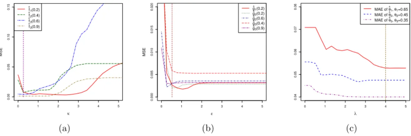
Figure 2: values of the mean-squared error for (a) ˆf_px0q with respect to κ, (b) ˆgpx0q with respect to ǫ.

(c) : Values of the mean-absolute error for ˆθn with respect to λ. The sample size is n “ 2000 for all

computations. The vertical line corresponds to the chosen value of κ (figure (a)), ǫ (figure (b)) and λ (figure (c)).

We shall settle the values of the constants κ, ǫ and λ involved in the penalty terms Vpx0, hq, Γ1phq and

Γ2pbq respectively, to compute the selected bandwidths. Since the calibrations of these tuning parameters

are carried out in the same fashion, we only describe the calibration for κ. Denote by ˆfκ the estimator

of f depending on the constant κ to be calibrated. We approximate the mean-squared error for the estimator ˆfκ, defined by MSEp ˆfκpx0qq “ Erp ˆfκpx0q ´ fpx0qq2s, over 100 Monte-Carlo runs, for different

possible valuestκ1, . . . , κKu of κ, for the three densities f1, f2, f3calculated at several test points x0. We

choose a value for κ that leads to small risks in all investigated cases. Figure 2(a)shows that κ“ 0.26 is an acceptable choice even if other values can be also convenient. Similarly, we set ǫ“ 0.52 and λ “ 4 (see Figure2(b) and2(c)) for the calibrations of ǫ and λ.

5.3

Simulation results

5.3.1 Estimation of the mixing proportion θ

We compare our estimator ˆθnwith the histogram-based estimator ˆθnNg-Mproposed in [24] and the estimator

ˆ θS

n introduced in [28]. Boxplots in Figure 3 represent the absolute errors of ˆθn, ˆθNg-Mn and ˆθnS, labeled

respectively by ”Sym-Ker”, ”Histogram” and ”Bootstrap”. The estimators ˆθnand ˆθNg-Mn have comparable

performances, and outperform ˆθS n. ● ● ● ● ● ● ●

Sym−Ker Histogram Boostrap

0.00 0.05 0.10 0.15 θ1 = 0. 65 ● ● ● ●

Sym−Ker Histogram Boostrap

0.00 0.05 0.10 0.15 θ2 = 0. 45 ● ● ● ● ● ● ●

Sym−Ker Histogram Boostrap

0.00 0.02 0.04 0.06 0.08 0.10 0.12 θ3 = 0. 35

5.3.2 Estimation of the target density f

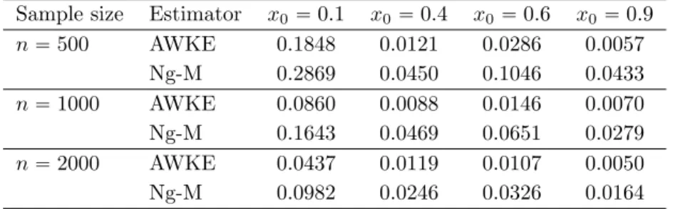
We present in Tables 1, 2 and 3 the mean-squared error (MSE) for the estimation of f according to the three different models and the different sample sizes introduced in Section 5.1. The MSEs’ are approximated over 100 Monte-Carlo replications. We shall choose the estimation points (to compute the pointwise risk): we propose x0 P t0.1, 0.4, 0.6, 0.9u. The choices of x0“ 0.4 and x0“ 0.6 are standard.

The choices of x0“ 0.1 and x0“ 0.9 allows to test the performance of ˆf close to the boundaries of the

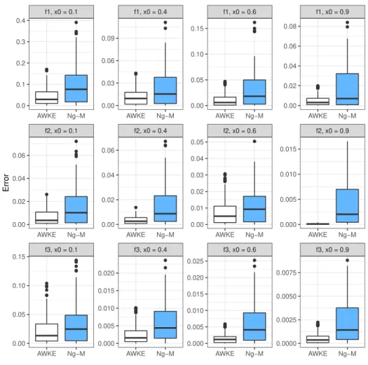
domain of definition of f and g. We compare our estimator ˆf with the randomly weighted estimator proposed in Nguyen and Matias [23]. In the sequel, the label ”AWKE” (Adaptive Weighted Kernel Estimator) refers to our estimator ˆf, whose bandwidth is selected by the Goldenshluger-Lepski method and ”Ng-M” refers to the one proposed by [23]. Resulting boxplots are displayed in Figure4for n“ 2000.

Sample size Estimator x0“ 0.1 x0“ 0.4 x0“ 0.6 x0“ 0.9

n“ 500 AWKE 0.1848 0.0121 0.0286 0.0057 Ng-M 0.2869 0.0450 0.1046 0.0433 n“ 1000 AWKE 0.0860 0.0088 0.0146 0.0070 Ng-M 0.1643 0.0469 0.0651 0.0279 n“ 2000 AWKE 0.0437 0.0119 0.0107 0.0050 Ng-M 0.0982 0.0246 0.0326 0.0164

Table 1: mean-squared error of the reconstruction of f1, for our estimator ˆf (AWKE), and for the

estimator of Nguyen and Matias [23] (Ng-M).

Sample size Estimator x0“ 0.1 x0“ 0.4 x0“ 0.6 x0“ 0.9

n“ 500 AWKE 0.0453 0.0136 0.0297 0.0024 Ng-M 0.0560 0.0540 0.0306 0.0138 n“ 1000 AWKE 0.0190 0.0061 0.0237 0.0006 Ng-M 0.0277 0.0209 0.0123 0.0069 n_{“ 2000} AWKE 0.0063 0.0036 0.0075 0.0001 Ng-M 0.0164 0.0159 0.0113 0.0038

Table 2: mean-squared error of the reconstruction of f2, for our estimator ˆf (AWKE), and for the

estimator of Nguyen and Matias [23] (Ng-M).

Sample size Estimator x0“ 0.1 x0“ 0.4 x0“ 0.6 x0“ 0.9

n_{“ 500} AWKE 0.0806 0.0096 0.0045 0.0016 Ng-M 0.1308 0.0247 0.0207 0.0096 n_{“ 1000} AWKE 0.0321 0.0054 0.0029 0.0010 Ng-M 0.0566 0.0106 0.0096 0.0060 n_{“ 2000} AWKE 0.0239 0.0025 0.0015 0.0005 Ng-M 0.0342 0.0059 0.0062 0.0021

Table 3: mean-squared error of the reconstruction of f3, for our estimator ˆf (AWKE), and for the

estimator of Nguyen and Matias [23] (Ng-M).

Tables1,2,3and boxplots show that our estimator outperforms the one of [23]. Notice that the errors are relatively large at the point x0“ 0.1, for both estimators, which was expected (boundary effect).

● ● ● ● ● ● ● ● ● ● ● ● ● ● ● ● ● ● ● ● ● ● ● ● ● ● ● ● ● ● ● ● ● ● ● ● ● ● ● ● ● ● ● ● ● ● ● ● ● ● ● ● ● ● ● ● ● ● ● ● ● ● ● ● ● ● ● ● ● ● ● ● ● ● f3, x0 = 0.1 f3, x0 = 0.4 f3, x0 = 0.6 f3, x0 = 0.9 f2, x0 = 0.1 f2, x0 = 0.4 f2, x0 = 0.6 f2, x0 = 0.9 f1, x0 = 0.1 f1, x0 = 0.4 f1, x0 = 0.6 f1, x0 = 0.9

AWKE Ng−M AWKE Ng−M AWKE Ng−M AWKE Ng−M

AWKE Ng−M AWKE Ng−M AWKE Ng−M AWKE Ng−M

AWKE Ng−M AWKE Ng−M AWKE Ng−M AWKE Ng−M

0.00 0.02 0.04 0.06 0.08 0.000 0.005 0.010 0.015 0.0000 0.0025 0.0050 0.0075 0.00 0.05 0.10 0.15 0.00 0.01 0.02 0.03 0.04 0.05 0.000 0.005 0.010 0.015 0.020 0.025 0.00 0.03 0.06 0.09 0.00 0.02 0.04 0.06 0.000 0.005 0.010 0.015 0.020 0.0 0.1 0.2 0.3 0.4 0.00 0.02 0.04 0.06 0.00 0.05 0.10 0.15 Error

Figure 4: errors for the estimation of f1, f2 and f3 for x0P t0.1, 0.4, 0.6, 0.9u and sample size n “ 2000.

6

Proofs

In the sequel, the notations ˜P_{, ˜}E_{and ˜}V_{ar respectively denote the probability, the expectation and the} variance associated with X1, . . . , Xn, conditionally on the additional random sample Xn`1, . . . , X2n.

6.1

Proof of Proposition

1

Let ρą 1, introduce the event

Ωρ“ ! ρ´1γď ˆγ ď ργ). such as ˆ fhpx0q ´ fpx0q “ `<sub>ˆ</sub> fhpx0q ´ fpx0q˘1Ωρ ` `_ˆ fhpx0q ´ fpx0q˘1Ωc ρ. (20)

We first evaluate the term `_ˆ

fhpx0q ´ fpx0q˘1Ωρ. Suppose now that we are on Ωρ, then for any

x0P r0, 1s, we have `<sub>ˆ</sub> fhpx0q ´ fpx0q ˘2 ď 3´`_ˆ fhpx0q ´ Kh‹ ˇfpx0q ˘2 ``Kh‹ ˇfpx0q ´ ˇfpx0q ˘2 ``_ˇ fpx0q ´ fpx0q ˘2¯ , (21) where we define ˇ fpxq “ wp˜θn,ˆgpxqqgpxq “ 1 1´ ˜θn ˜ 1´ _ˆθ˜n gpxq ¸ gpxq. Note that by definition of ˇf, we have Kh‹ ˇfpx0q “ ˜E“fˆhpx0q‰. Hence,

`<sub>ˆ</sub> fhpx0q ´ Kh‹ ˇfpx0q ˘2 “`_ˆ fhpx0q ´ ˜E “_ˆ fhpx0q ‰˘2 .

It follows that ˜ E”`_fˆ_{hpx0q ´ ˜}E“_fˆ_hpx0q‰˘2ı_{“ ˜}V_ar´ ˆ_fhpx0q¯_{“ ˜}V_ar ˜ 1 n n ÿ i“1 wp˜θn,ˆgpXiqqKhpx0´ Xiq ¸ “ 1 nV˜ar ´ wp˜θn,ˆgpX1qqKhpx0´ X1q ¯ ď 1 nE˜ „_´ wp˜θn,gˆpX1qqKhpx0´ X1q ¯2 . On the other hand, for all iP t1, . . . , nu, thanks to (A4) and (A2),

w_p˜θn,ˆgpXiqqKhpx0´ Xiq “ 1 1´ ˜θn ˜ 1´_ˆθ˜n gpXiq ¸ Khpx0´ Xiq ď 2 δ ˜ 1` θ˜n |ˆgpXiq| ¸ Khpx0´ Xiq ď 2 δ ˆ 1` 1_ˆ γ ˙ Khpx0´ Xiq ď 4 δˆγKhpx0´ Xiq. (22)

Indeed, as we use compactly supported kernel to construct the estimator ˆfh, condition αn ď h´1 in

(A5) ensures that_`ˆgpXiq˘´1Khpx0´ Xiq is upper bounded by ˆγ´1Khpx0´ Xiq even though we have no

observation in the neighbourhood of x0.

Moreover, since ˆγě ρ´1_{γ on Ω}

ρ, we have that wp˜θn,ˆgpXiqq ď 4ρδ´1γ´1. Thus we obtain

˜ E”`fˆhpx0q ´ ˜E “_ˆ fhpx0q ‰˘2ı ď 16ρ 2 δ2_γ2_nE˜ ” K2 hpx0´ X1q ı ď 16ρ 2 }K}2 2}g}_8,Vnpx0q δ2_γ2_nh . (23)

For the last two terms of (21), we apply the following proposition:

Proposition 2. Assume (A1) and (A3). On the set Ωρ, we have the following results for any x0P r0, 1s

`<sub>ˇ</sub> fpx0q ´ fpx0q ˘2 ď C1δ´2γ´2}ˆg ´ g} 2 8,Vnpx0q` C2δ ´6ˇ ˇ ˜θn´ θ ˇ ˇ 2 , (24) `Kh‹ ˇfpx0q ´ ˇfpx0q ˘2 ď 6 }Kh‹ f ´ f} 2 8,Vnpx0q` C3δ ´2_γ´2_{}ˆg ´ g}}2 8,Vnpx0q` C4δ ´6ˇ ˇ ˜θn´ θ ˇ ˇ 2 , (25) where C1 and C2 respectively depend on ρ and }g}_8,Vnpx0q, C3 depends on ρ and }K}1 and C4 depends

on }g}_8,Vnpx0q and}K}1.

Combining (23), (24) and (25), we obtain

E ” `<sub>ˆ</sub> fhpx0q ´ fpx0q ˘2 1Ωρ ı ď 18 }Kh‹ f ´ f} 2 8,Vnpx0q` 3pC1` C3qδ ´2<sub>γ</sub>´2<sub>E“ }ˆg ´ g}</sub>2 8,Vnpx0q ‰ ` 3pC2` C4qδ´6E “ˇ ˇ ˜θn´ θ ˇ ˇ 2 ‰ `48ρ 2_}K}2 2}g}8,Vnpx0q δ2_γ2_nh .

It remains to study the risk bound on Ωc

ρ. To do so, we successively apply the following lemmas whose

proofs are postponed to the end of Theorem1’s proof.

Lemma 3. Suppose that Assumption (A3) is satisfied. Then we have for ρą 1 P´_Ωc ρ ¯ ď Cg,ρexp ! ´plog nq3{2)_,

with Cg,ρ a positive constant depending on g and ρ.

Lemma 4. Assume (A2) and (A5). For any hP Hn, we have

E”`fˆhpx0q ´ fpx0q ˘2 1Ωc ρ ı ď C4˚ δ2_n2, with C˚

4 a positive constant depending on}f}_8,Vnpx0q,}K}8, g and ρ.

6.2

Proof of Lemma

2

First, we prove that ˆg_bsymhas the same distribution as ˆrb. First, Yi has the same distribution as 2´ Yi.

Thus, ˆg_bsymhas the same distribution as xÞÑ n´1řn

i“1Lbpx ´ Yiq. It is thus sufficient to show that Yi

has the same distribution as Ri. To this aim, let ϕ be a measurable bounded function defined on R. We

compute

E<sub>rϕpYiqs “ ErErϕpXiq|εis1tǫ1“1us ` ErErϕp2 ´ Xiq|εis1tǫ1“´1us,</sub> “ 1<sub>2</sub>`ErϕpXiqs ` Erϕp2 ´ Xiqs˘ , “ 1<sub>2</sub> ˜ ż1 0 ϕpxqgpxqdx ` ż1 0 ϕp2 ´ xqgpxqdx ¸ , “ 1₂ ˜ ż1 0 ϕ_{pxqgpxqdx `} ż2 1 ϕ_{pxqgp2 ´ xqdx} ¸ , “ ż2 0 ϕ_{pxqrpxqdx “ ErϕpR}iqs.

This allows us to obtain the first assertion of the lemma.

We prove now (18). Under the identifiability condition, we have θ“ gpxq for all x P r1 ´ δ, 1s. Hence we have |ˆθn,b´ θ| “ ˇ ˇ ˇ ˇ ˇ 1 δ ż1 1_´δ ˆ g_bsym_{pxqdx ´} 1 δ ż1 1_´δ g_pxqdx ˇ ˇ ˇ ˇ ˇ “1 δ ˇ ˇ ˇ ˇ ˇ ż1 1_´δpˆg sym b pxq ´ gpxqqdx ˇ ˇ ˇ ˇ ˇ ď 1 δ ż1 1_´δ ˇ ˇˆg_bsym_{pxq ´ gpxq}ˇ ˇdx ď 1 δ ż1 1_´δ › ›ˆgsym_{b ´ g}› › 8,r1´δ,1sdx “› ›ˆg_bsym´ g› › 8,r1´δ,1s.

Moreover, thanks to the Markov Inequality P´ ˜_{θn,b‰ ˆθn,b}¯ _{“ P} ˜ ˆ θn,bR „ δ 2,1´ δ 2 ¸ ď P ˆ |ˆθn,b´ θ| ą δ 2 ˙ ď_δ42E ” |ˆθn,b´ θ|2 ı , which is (19). This concludes the proof of Lemma2.

6.3

Proof of Proposition

2

Let us introduce the function ˜ fpxq :“ wp˜θn, gpxqqgpxq “ 1 1´ ˜θn ˜ 1´ θ˜n g_pxq ¸ gpxq. (26)

Then we have for x0P r0, 1s

`ˇ fpx0q ´ fpx0q˘ 2 ď 2´`ˇ fpx0q ´ ˜fpx0q˘ 2 ``˜ fpx0q ´ fpx0q˘ 2¯ .

For the first term, on Ωρ“ ρ´1γď ˆγ ď ργ( we have, by using (A4), `_ˇ fpx0q ´ ˜fpx0q ˘2 “´wp˜θn,gˆpx0qqgpx0q ´ wp˜θn, gpx0qqgpx0q ¯2 “ ¨ ˝ 1 1´ ˜θn ˜ 1´ θ˜n ˆ g_px0q ¸ ´ 1 1´ ˜θn ˜ 1´ θ˜n g_px0q ¸˛ ‚ 2 |gpx0q|2 “ θ˜ 2 n p1 ´ ˜θnq2 ˆ ₁ ˆ gpx0q´ 1 gpx0q ˙2 |gpx0q|2 ď 4 δ2 ˆ ˆg_px0q ´ gpx0q ˆ gpx0qgpx0q ˙2 |gpx0q|2 ď 4ρ2 δ´2γ´2}ˆg ´ g}2_8,Vnpx0q. (27)

Moreover, thanks to (A1), `˜ fpx0q ´ fpx0q˘ 2 “´wp˜θn, gpx0qqgpx0q ´ wpθ, gpx0qqgpx0q ¯2 “ ¨ ˝ 1 1´ ˜θn ˜ 1´ θ˜n g<sub>px</sub>0q ¸ gpx0q ´ 1 1´ θ ˜ 1´ θ g<sub>px</sub>0q ¸ gpx0q ˛ ‚ 2 “ ¨ ˝ 1 1´ ˜θn ´ 1 1´ θ ` ˜ θ 1´ θ ´ ˜ θn 1´ ˜θn ¸ 1 g_px0q ˛ ‚ 2 |gpx0q|2 “ |gpx0q| 2 p1 ´ θq2_{p1 ´ ˜θ} nq2 ˜ ˜ θn´ θ ` θ<sub>´ ˜</sub>θn g<sub>px</sub>0q ¸2 ď 4}g} 2 8,Vnpx0q δ4 ˜ ˜ θn´ θ ` θ´ ˜θn g_px0q ¸2 ď 16 }g}2_8,Vnpx0qδ ´6ˇ ˇ ˜θn´ θ ˇ ˇ 2 . (28)

Thus we obtain by gathering (27) and (28),

`ˇ fpx0q ´ fpx0q˘ 2 ď 8ρ2 δ´2γ´2}ˆg ´ g}2<sub>8,V</sub>npx0q` 32 }g} 2 8,Vnpx0qδ ´6ˇ ˇ ˜θn´ θ ˇ ˇ 2 . Next, the term`Kh‹ ˇfpx0q ´ ˇfpx0q

˘2

can be treated by studying the following decomposition `Kh‹ ˇfpx0q ´ ˇfpx0q ˘2 ď 3 ˆ `Kh‹ ˇfpx0q ´ Kh‹ ˜fpx0q ˘2 ``Kh‹ ˜fpx0q ´ Kh‹ fpx0q ˘2 ``Kh‹ fpx0q ´ ˇfpx0q ˘2 ˙ “: 3`A1` A2` A3q.

For term A1, we have by using (27)

A1“`Kh‹ p ˇf´ ˜fqpx0q

˘2 “

ˆż

Khpx0´ uqp ˇfpuq ´ ˜fpuqqdu

˙2

ď ˆż

|Khpx0´ uq|| ˇfpuq ´ ˜fpuq|du

˙2 ď 4ρ2 δ´2γ´2}ˆg ´ g}2_8,Vnpx0q ˆż |Khpx0´ uq|du ˙2 ď 4ρ2_δ´2_γ´2_}K}2 1}ˆg ´ g} 2 8,Vnpx0q.

By using (28) and following the same lines as for A1, we obtain A2“`Kh‹ p ˜f´ fqpx0q˘ 2 ď 16 }g}2_8,Vnpx0qδ ´6_}K}2 1 ˇ ˇ ˜θn´ θ ˇ ˇ 2 . For A3, using the upper bound obtained as above forp ˇfpx0q ´ fpx0qq2, we have

A3ď 2`Kh‹ fpx0q ´ fpx0q ˘2 ` 2`f px0q ´ ˇfpx0q ˘2 ď 2 }Kh‹ f ´ f} 2 8,Vnpx0q` 16ρ 2 δ´2γ´2}ˆg ´ g}2_8,Vnpx0q` 64 }g} 2 8,Vnpx0qδ ´6ˇ ˇ ˜θn´ θ ˇ ˇ 2 . Finally, combining all the terms A1, A2 and A3, we obtain (25). This ends the proof of Proposition2.

6.4

Proof of Theorem

1

Suppose that we are on Ωρ. Let ˆf be the adaptive estimator defined in (8), we have for any x0P r0, 1s,

`<sub>ˆ</sub> fpx0q ´ fpx0q ˘2 ď 2´`_ˆ fpx0q ´ ˇfpx0q ˘2 ``_ˇ fpx0q ´ fpx0q ˘2¯

The second term is controlled by (24) of Proposition 2. Hence it remains to handle with the first term. For any hP Hn, we have

`<sub>ˆ</sub> fpx0q ´ ˇfpx0q ˘2 ď 3´`_ˆ fˆ_hpx0qpx0q ´ ˆf_h,hˆ px0q ˘2 ``<sub>ˆ</sub> fˆ<sub>hpx0q,h</sub>px0q ´ ˆfhpx0q ˘2 ``_ˆ fhpx0q ´ ˇfpx0q ˘2¯ “ 3´`<sub>ˆ</sub> fˆ<sub>hpx</sub>0qpx0q ´ ˆfh,hˆ px0q ˘2 ´ V px0, ˆhq ` `<sub>ˆ</sub> fˆ<sub>hpx</sub>0q,hpx0q ´ ˆfhpx0q ˘2 ´ V px0, hq `V px0, ˆhq ` V px0, hq ` `<sub>ˆ</sub> fhpx0q ´ ˇfpx0q ˘2¯ ď 3´A<sub>px</sub>0, ˆhq ` Apx0, hq ` V px0, ˆhq ` V px0, hq ` `_ˆ fhpx0q ´ ˇfpx0q ˘2¯ ď 6Apx0, hq ` 6V px0, hq ` 3 `<sub>ˆ</sub> fhpx0q ´ Kh‹ ˇfpx0q ˘2 ` 3`Kh‹ ˇfpx0q ´ ˇfpx0q ˘2 . (29) Next, we have Apx0, hq “ max h1<sub>PH</sub> n ! `_ˆ fh,h1px₀q ´ ˆf_h1px₀q˘ 2 ´ V px0, h1q ) ` ď 3 max h1<sub>PH</sub> n ! `ˆ fh,h1px₀q ´ K_h1‹ pK_h‹ ˇfqpx₀q˘ 2 ``ˆ fh1px<sub>0</sub>q ´ K<sub>h</sub>1‹ ˇfpx<sub>0</sub>q˘ 2 ``Kh1‹ pK_h‹ ˇfqpx₀q ´ K_h1‹ ˇfpx₀q˘ 2 ´Vpx₃0, h1q * ` ď 3`Bphq ` D1` D2˘ , where Bphq “ max h1_PH n ´ Kh1‹ pK_h‹ ˇfqpx₀q ´ K_h1‹ ˇfpx₀q ¯2 D1“ max h1_PH n " `<sub>ˆ</sub> fh1px<sub>0</sub>q ´ K<sub>h</sub>1‹ ˇfpx<sub>0</sub>q˘ 2 ´Vpx0, h1q 6 * ` D2“ max h1_PH n " `ˆ fh,h1px<sub>0</sub>q ´ K<sub>h</sub>1‹ pK<sub>h</sub>‹ ˇfqpx<sub>0</sub>q˘ 2 ´Vpx<sub>6</sub>0, h1q * ` . Since B_{phq “ max} h1_PH n ´ Kh1‹ pK_h‹ ˇfqpx₀q ´ K_h1‹ ˇfpx₀q ¯2 “ max h1_PH n ´ Kh1‹ pK_h‹ ˇf ´ ˇfqpx₀q ¯2 ď }K}21 sup tPVnpx0q ˇ ˇKh‹ ˇfptq ´ ˇfptq ˇ ˇ 2 ,

then we can rewrite (29) as ´ ˆ_{fpx0q ´ ˇfpx0q}¯2 ď 18D1` 18D2` 6V px0, hq ` 3 `_ˆ fhpx0q ´ Kh‹ ˇfpx0q ˘2 ` p18 }K}21` 3q sup tPVnpx0q ˇ ˇKh‹ ˇfptq ´ ˇfptq ˇ ˇ 2 . (30) The last two terms of (30) are controlled by (23) and (25) of Proposition 2. Hence it remains to deal with terms D1 and D2.

For D1, we recall that Kh‹ ˇfpx0q “ ˜E“fˆhpx0q‰ and

˜ E_{rD1s “ ˜}E « max hPHn " ´ ˆ_{fhpx0q ´ Kh‹ ˇfpx0q}¯2 ´Vpx₆0, hq * ` ff ď ÿ hPHn ˜ E «<sub>"</sub> ´ ˆ<sub>fhpx0q ´ ˜</sub>E“fˆhpx0q ¯2 ´Vpx<sub>6</sub>0, hq * ` ff ď ÿ hPHn ż`8 0 ˜ P ˜ " `ˆ fhpx0q ´ ˜E“fˆhpx0q˘ 2 ´Vpx0, hq 6 * ` ą u ¸ du ď ÿ hPHn ż`8 0 ˜ P ˜ ˇ ˇ ˆf_hpx0q ´ ˜E “_ˆ fhpx0q ˇ ˇą c Vpx0, hq 6 ` u ¸ du. (31)

Now let us introduce the sequence of i.i.d. random variables Z1, . . . , Zn where we set

Zi“ wp˜θn,ˆgpXiqqKhpx0´ Xiq. Then we have ˆ fhpx0q ´ ˜E “_ˆ fhpx0q‰ “ 1 n n ÿ i“1 `Zi´ ˜ErZis˘.

Moreover, we have by (22) and (23)

|Zi| “ |wp˜θn,gˆpXiqqKhpx0´ Xiq| ď 4}K}₈ hδˆγ “: b, and ˜ E_“Z12_{‰ “ ˜E}”_{wp˜θn,gˆpXiqq}2_K2 hpx0´ Xiq ı ď16}K} 2 2}g}8,Vnpx0q hδ2_ˆγ2 “: v.

Applying the Bernstein inequality (cf. Lemma 2 of Comte and Lacour [9]), we have for any uą 0, ˜ P ˜ ˇ ˇ ˆfhpx0q ´ ˜E “_ˆ fhpx0q ˇ ˇą c V_px0, hq 6 ` u ¸ “ ˜P ˜ ˇ ˇ ˇ 1 n n ÿ i“1 `Zi´ ˜ErZis ˘ˇ_ˇ ˇ ą c V_px0, hq 6 ` u ¸ ď 2 max $ & % exp ˜ ´<sub>4v</sub>n ˆ V px<sub>6</sub>0, hq` u ˙¸ ,exp ˜ ´_4bn c Vpx0, hq 6 ` u ¸, . -ď 2 max $ & % exp ˆ ´_24vn V_px0, hq ˙ exp ˆ ´nu_4v ˙ ,exp ˜ ´_8bn c V_px0, hq 6 ¸ exp ˜ ´n ? u 8b ¸, .

-On the other hand, by the definition of Vpx0, hq we have

n 24vVpx0, hq “ nhˆγ2_δ2 384ρ}K}22}g}8,Vnpx0q ˆκ}K} 2 1}K} 2 2}g}_8,Vnpx0q ˆ γ2_nh logpnq “ κδ2 }K}21 384ρ logpnq ě κδ2 384ρlogpnq. If we choose κ such that κδ

2

384ρ ě 2, we get n

Moreover, using the assumption that ˆγnhě log3pnq we have n 8b c Vpx0, hq 6 “ nhˆγδ 32?6}K}₈ ˆ }K}1}K}2 b κ}g}_8,Vnpx0qlogpnq ˆ γ?nh “δ}K}1}K}2}g} 1{2 8,Vnpx0q 32?6}K}₈ a κnhlogpnq ě δ}K}1}K}2 32?6ρ1_{2γ1_{2}K} 8 ? κlog2pnq ě 2 logpnq, if δ_}K}1}K}2 32?6ρ1_{2γ1_{2}K} 8 ? κlogpnq ě 2

which automatically holds for well-chosen value of κ, and n large enough. Then we have by using the conditions ρ´1_{γď ˆγ and h ě 1{n,} ˜ E_{rD1s ď} ÿ hPHn ż`8 0 2n´2max $ & % exp ˆ ´nu<sub>4v</sub> ˙ ,exp ˜ ´n ? u 8b ¸, . -du ď 2n´2 ÿ hPHn ż`8 0 max $ & % exp ¨ ˝´nh δ2_γˆ2 64}K}22}g}8,Vnpx0q u ˛ ‚,exp ˜ ´nh δˆγ 32}K}₈ ? u ¸, . -du ď 2n´2 ÿ hPHn ż`8 0 max $ & % exp ¨ ˝´nh δ2<sub>γ</sub>2 64ρ2<sub>}K}</sub>2 2}g}<sub>8,V</sub>npx0q u ˛ ‚,exp ˜ ´nh δγ 32ρ}K}8 ? u ¸, . -du ď 2n´2 ÿ hPHn ż`8 0 max!e´π1u , e´π2?u ) du_{ď 2n}´2 ÿ hPHn max # 1 π1 , 2 π2 2 + . with π1:“ δ2_γ2 64ρ2_}K}2 2}g}8,Vnpx0q and π2:“ δγ 32ρ}K}₈. Since cardpHnq ď n, we finally obtain

˜

E_{rD1s ď C5δ}´2_γ´2_n´1_{, (32)}

where C5 is a positive constant depending on}g}_8,Vnpx0q,}K}8,}K}2 and ρ.

Similarly, we introduce Ui“ wp˜θn,gˆpXiqqKh1‹ K_hpx₀´ X_iq for i “ 1, . . . , n. Then,

ˆ fh,h1px₀q ´ K_h1‹ pK_h‹ ˇfqpx₀q “ ˆf_h,h1px₀q ´ ˜E “_ˆ fh,h1px₀q‰ “ 1 n n ÿ i“1 `Ui´ ˜ErUis˘, and |Ui| ď 4}K}1}K}8 h1_δˆγ “: ¯b, and E˜“U 2 1‰ ď 16}K}21}K} 2 2}g}_8,Vnpx0q h1_δ2_ˆγ2 “: ¯v.

Following the same lines as for obtaining (32), we get by using Bernstein inequality ˜

E_{rD2s ď C6δ}´2_γ´2_n´1_{, (33)}

with C6 a positive constant depends on}g}_8,Vnpx0q,}K}8,}K}1,}K}2 and ρ.

Finally, combining (30), (32), (33) and successively applying Lemma 3 and Lemma 4 allow us to conclude the result stated in Theorem 1.

6.5

Proof of Corollary

1

Assume that Assumptions (A6) and (A7) are fulfilled. According to Proposition 1.2 of Tsybakov [30], we get for all x0P r0, 1s

|Kh‹ fpx0q ´ fpx0q| ď C7Lhβ,

where C a constant depending on K and L. Taking

h“ L´1{β_Λ´1{β n , Λn“ L´1{p2β`1q ˜ δ2<sub>γ</sub>2<sub>n</sub> log n ¸β{p2β`1q , we get logpnq δ2_γ2_nh “ Λ´2n . Hence, we obtain min hPHn " }Kh‹ f ´ f} 2 8,Vnpx0q` logpnq δ2<sub>γ</sub>2<sub>nh</sub> * ď pC2 7` 1qL 2{p2β`1q ˜ δ2γ2n log n ¸´2β{p2β`1q . (34)

Finally, since we also assume (10), gathering (9) and (34), we obtain

E ” `<sub>ˆ</sub> f<sub>px</sub>0q ´ fpx0q ˘2ı ď C8 ˆ log n n ˙ 2β 2β`1 ,

where C8is a constant depending on K,}f}_8,Vnpx0q, g, δ, γ, ρ, L and β. This ends the proof of Corollary

1.

6.6

Proofs of technical lemmas

Lemma 3 is a consequence of (5). Indeed, assume that condition (A3) is satisfied, then we have for all tP Vnpx0q, |ˆgptq ´ gptq| ď ν|ˆgptq| with probability 1 ´ Cg,νexp` ´ plog nq3{2˘.

This implies, p1 ` νq´1|gptq| ď |ˆgptq| ď p1 ´ νq´1|gptq|. Since γ“ inf tPVnpx0q |gptq| and ˆγ “ inf tPVnpx0q

|ˆgptq|, by using (5) and taking ν “ ρ ´ 1, ν “ 1 ´ ρ´1_{, we obtain}

with probability 1´ Cg,νexp` ´ plog nq3{2˘, p1 ` νq´1γď ˆγ ď p1 ´ νq´1γ which completes the proof of

Lemma 3.

6.6.2 Proof of Lemma 4

We have for any x0P r0, 1s,

E”`ˆ fhpx0q ´ fpx0q˘ 2 1Ωc ρ ı ď 2E“| ˆfhpx0q|21Ωc ρ‰ ` 2 }f} 2 8,Vnpx0qPpΩ c ρq.

Using Assumptions (A6) and (22), we obtain

E_{“| ˆfhpx0q|}2_1Ωc ρ‰ “ E » – ˇ ˇ ˇ ˇ ˇ 1 nh n ÿ i“1 wp˜θn,gˆpXiqqK ˆ x0´ Xi h ˙ˇ_ˇ ˇ ˇ ˇ 2 1Ωc ρ fi fl ď 16 δ2E » – ˇ ˇ ˇ ˇ ˇ 1 ˆ γnh n ÿ i“1 Kˆ x0´ Xi h ˙ˇ_ˇ ˇ ˇ ˇ 2 1Ωc ρ fi fl ď 16}K} 2 8 δ2 n2 plog nq6PpΩ c ρq.

Finally, we apply Lemma3to establish the following bound E”`fˆhpx0q ´ fpx0q ˘2 1Ωc ρ ı ď Cg,ρ ˜ 16}K}2<sub>8</sub> δ2 n2 plog nq6 ` 2 }f} 2 8,Vnpx0q ¸ exp!´plog nq3{2) ď 16Cg,ρ}K} 2 8}f} 2 8,Vnpx0q δ2 1 n2,

which ends the proof of Lemma4.

Acknowledgment

We are very grateful to Catherine Matias for interesting discussions on mixture models. The research of the authors is partly supported by the french Agence Nationale de la Recherche (ANR-18-CE40-0014 projet SMILES) and by the french R´egion Normandie (projet RIN AStERiCs 17B01101GR).

References

[1] Yoav Benjamini and Yosef Hochberg. Controlling the false discovery rate: a practical and powerful approach to multiple testing. Journal of the Royal statistical society: series B (Methodological), 57(1):289–300, 1995.

[2] Karine Bertin, Claire Lacour, and Vincent Rivoirard. Adaptive pointwise estimation of conditional density function. preprint arXiv:1312.7402, 2013.

[3] Karine Bertin, Claire Lacour, and Vincent Rivoirard. Adaptive pointwise estimation of conditional density function. Ann. Inst. H. Poincar Probab. Statist., 52(2):939–980, 05 2016.

[4] C. Butucea. Two adaptive rates of convergence in pointwise density estimation. Math. Methods Statist., 9(1):39–64, 2000.

[5] Alain Celisse and St´ephane Robin. A cross-validation based estimation of the proportion of true null hypotheses. Journal of Statistical Planning and Inference, 140(11):3132–3147, 2010.

[6] Ga¨elle Chagny. Penalization versus goldenshluger- lepski strategies in warped bases regression. ESAIM: Probability and Statistics, 17:328–358, 2013.

[7] Micha¨el Chichignoud, Van Ha Hoang, Thanh Mai Pham Ngoc, Vincent Rivoirard, et al. Adaptive wavelet multivariate regression with errors in variables. Electronic journal of statistics, 11(1):682– 724, 2017.

[8] F. Comte, S. Ga¨ıffas, and A. Guilloux. Adaptive estimation of the conditional intensity of marker-dependent counting processes. Ann. Inst. Henri Poincar´e Probab. Stat., 47(4):1171–1196, 2011. [9] F. Comte and C. Lacour. Anisotropic adaptive kernel deconvolution. Ann. Inst. Henri Poincar´e

Probab. Stat., 49(2):569–609, 2013.

[10] Fabienne Comte. Estimation non-param´etrique. Spartacus-IDH, 2015.

[11] Fabienne Comte, Valentine Genon-Catalot, and Adeline Samson. Nonparametric estimation for stochastic differential equations with random effects. Stochastic Processes and their Applications, 123(7):2522–2551, 2013.

[12] Fabienne Comte and Tabea Rebafka. Nonparametric weighted estimators for biased data. Journal of Statistical Planning and Inference, 174:104–128, 2016.

[13] Marie Doumic, Marc Hoffmann, Patricia Reynaud-Bouret, and Vincent Rivoirard. Nonparametric estimation of the division rate of a size-structured population. SIAM Journal on Numerical Analysis, 50(2):925–950, 2012.

[14] Bradley Efron, Robert Tibshirani, John D Storey, and Virginia Tusher. Empirical bayes analysis of a microarray experiment. Journal of the American statistical association, 96(456):1151–1160, 2001. [15] Christopher Genovese and Larry Wasserman. Operating characteristics and extensions of the false discovery rate procedure. Journal of the Royal Statistical Society: Series B (Statistical Methodology), 64(3):499–517, 2002.

[16] Evarist Gin´e and Richard Nickl. An exponential inequality for the distribution function of the kernel density estimator, with applications to adaptive estimation. Probab. Theory Related Fields, 143(3-4):569–596, 2009.

[17] Alexander Goldenshluger and Oleg Lepski. Bandwidth selection in kernel density estimation: orcale inequalities and adaptive minimax optimality. The Annals of Statistics, 39(3):1608–1632, 2011. [18] Peter J Huber. A robust version of the probability ratio test. The Annals of Mathematical Statistics,

pages 1753–1758, 1965.

[19] I. A. Ibragimov and R. Z. Has1 _{minski˘ı. An estimate of the density of a distribution. Zap. Nauchn.}

Sem. Leningrad. Otdel. Mat. Inst. Steklov. (LOMI), 98:61–85, 161–162, 166, 1980. Studies in math-ematical statistics, IV.

[20] Mette Langaas, Bo Henry Lindqvist, and Egil Ferkingstad. Estimating the proportion of true null hypotheses, with application to dna microarray data. Journal of the Royal Statistical Society: Series B (Statistical Methodology), 67(4):555–572, 2005.

[21] Oleg Lepski et al. Multivariate density estimation under sup-norm loss: oracle approach, adaptation and independence structure. The Annals of Statistics, 41(2):1005–1034, 2013.

[22] Haoyang Liu and Chao Gao. Density estimation with contaminated data: Minimax rates and theory of adaptation. arXiv preprint arXiv:1712.07801, 2017.

[23] Van Hanh Nguyen and Catherine Matias. Nonparametric estimation of the density of the alternative hypothesis in a multiple testing setup. application to local false discovery rate estimation. ESAIM: Probability and Statistics, 18:584612, 2014.

[24] Van Hanh Nguyen and Catherine Matias. On efficient estimators of the proportion of true null hypotheses in a multiple testing setup. Scandinavian Journal of Statistics, 41(4):1167–1194, 2014. [25] Patricia Reynaud-Bouret, Vincent Rivoirard, Franck Grammont, and Christine Tuleau-Malot.

Goodness-of-fit tests and nonparametric adaptive estimation for spike train analysis. The Jour-nal of Mathematical Neuroscience, 4(1):1, 2014.

[26] St´ephane Robin, Avner Bar-Hen, Jean-Jacques Daudin, and Laurent Pierre. A semi-parametric approach for mixture models: Application to local false discovery rate estimation. Computational Statistics & Data Analysis, 51(12):5483–5493, 2007.

[27] Eugene F Schuster. Incorporating support constraints into nonparametric estimators of densities. Communications in Statistics-Theory and methods, 14(5):1123–1136, 1985.

[28] John D Storey. A direct approach to false discovery rates. Journal of the Royal Statistical Society: Series B (Statistical Methodology), 64(3):479–498, 2002.

[29] Korbinian Strimmer. A unified approach to false discovery rate estimation. BMC bioinformatics, 9(1):303, 2008.

[30] Alexandre B Tsybakov. Introduction to Nonparametric Estimation. Springer series in Statistics. Springer, New York, 2009.