A Partial Approach to Model Checking
∗(Extended Abstract)
Patrice Godefroid
Pierre Wolper
Institut Montefiore, B28
Universit´e de Li`ege
4000 Li`ege Sart-Tilman, Belgium
Email: {god,pw}@montefiore.ulg.ac.be
Abstract
This paper presents a model-checking method for linear-time temporal logic that avoids the state ex-plosion due to the modelling of concurrency by in-terleaving. The method relies on the concept of Mazurkiewicz’s trace as a semantic basis and uses automata-theoretic techniques, including automata that operate on words of ordinality higher than ω.
1
Introduction
Model Checking [13, 29, 35, 44] is an effective and simple method for verifying that a concurrent program satisfies a temporal logic formula. It works on finite-state programs and proceeds by viewing the program as a structure for interpreting temporal logic and by evaluating the formula on that structure. It is much simpler than temporal deductive proofs and can be easily and effectively implemented.
It has been intensively studied for linear-time tem-poral logic [29, 44, 43] branching-time temtem-poral logic [13, 19, 18, 6] and temporal µ-calculi [20, 42, 14, 37]. It has been extended to probabilistic [41, 33, 44, 17] as well as real-time programs and logics [2, 3, 25]. It has been adapted to programs containing arbitrary num-bers of identical processes [12, 11, 21, 47, 28]. Meth-ods for making it applicable to very large systems have been investigated [10, 15, 16, 23]. Moreover, the re-sults from its experimental use have been very encour-aging [36, 5]. What more can be said about it? In spite of all its success, almost all work around model checking is based on a very wasteful idea: modelling concurrency by interleaving. Even if one is not in-clined to loose sleep about whether interleaving se-mantics are adequate for concurrency, it remains
unar-∗This work is supported by the Esprit Basic Research Action
SPEC (3096).
guably silly to investigate the concurrent execution of n events by exploring all n! interleavings of these events!
In this paper, we develop a simple method for ap-plying model checking without incurring the cost of modelling concurrency by interleaving. Our method yields results identical to those of methods based on interleaving semantics, it just avoids most of the as-sociated combinatorial explosion. It is quite orthog-onal to model checking based on partial-order logics [32, 27, 31]. Indeed, these logics are designed to be semantically more powerful. We are “only” more effi-cient. The idea that the cost of modelling concurrency by interleaving can be avoided in finite-state verifica-tion already appears in [34, 39, 40, 22]. We build upon this earlier work, specifically that of [22], and bring to it the full capabilities of model checking.
We study model checking for linear-time temporal logic and adopt the automata-theoretic approach of [44, 42, 46]. In this approach, the program is viewed as a collection of communicating automata on infinite words [7]. It can thus include arbitrary fairness con-ditions. The negation of the formula to be checked is then also converted to an automaton on infinite words and the verification can be done by simply checking that the product of the automata describing the pro-gram and the automaton corresponding to the nega-tion of the formula is nonempty. This is tradinega-tionally done by computing the product automaton which is where the cost of modelling concurrency by interleav-ing has to be paid.
In [22] it is shown that the global behavior of a set of communicating processes can be represented by an automaton which can be much smaller than the usual product automaton. The basic idea is to build an automaton that only accepts one interleaving of
each concurrent execution. The method is justified by using partial-order semantics, namely the concept of Mazurkiewicz’s trace [30] and the automaton is thus called a trace automaton. A trace automaton can be viewed as an automaton accepting at least one, but usually no more than one, interleaving for each trace (concurrent computation) of the concurrent pro-gram. Thus, together with the independence rela-tion on transirela-tions, this automaton fully represents the concurrent executions of the program. The practical benefit is that this automaton can be much smaller than the automaton representing all interleavings. The motivating idea behind the method presented here is that, in the automata-theoretic approach to model checking, the trace automaton could be used in place of the product automaton. Unfortunately, this is not directly the case. However, we are able to obtain such a result by using a new type of automaton. We consider automata operating on infinite words of ordinality higher than ω. Precisely, we define au-tomata operating on words of length ω × n, n ∈ ω.1
We study these automata and give an efficient algo-rithm to check whether such automata are nonempty. We then show that, when it is viewed as an ω × n-automaton, the trace automaton can be substituted for the product automaton in linear-time model check-ing. The efficiency of the method of [22] is thus fully available for model checking.
Finally, we conclude the paper with a comparison be-tween our contributions and related work.
2
Automata and Model Checking
We briefly recall the essential elements of the automata-theoretic approach to model checking. More details can be found in [44, 46] and in Chapter 4 of [38]. The problem we consider is the following. We are given a concurrent program P composed of n pro-cesses Pi, each described by a finite automaton Ai on
countably infinite words over an alphabet Σi. We are
also given a linear-time propositional temporal logic formula f . The model-checking problem is then to verify that all infinite behaviors of the program P sat-isfy the temporal formula f .
The automata we use for describing the processes Pi
are generalized B¨uchi automata2, i.e. tuples A =
(Σ, S, ∆, s0,F), where
1Interestingly, a related type of automata on ordinals was
used by B¨uchi [9, 8] to study the decidability of the monadic theory of the ordinals.
2
Generalized B¨uchi automata differ from B¨uchi automata [7] in that they have a set of sets of accepting states rather than just one set of accepting states.
• Σ is an alphabet, • S is a set of states,
• ∆ ⊆ S × Σ × S is a transition relation, • s0∈ S is the starting state, and
• F = {F1, . . . , Fk} ⊆ 2Sis a set of sets of accepting
states.
Generalized B¨uchi automata are used to define lan-guages of ω-words, i.e. functions from the ordinal ω to the alphabet Σ. Intuitively, a word is accepted by a Generalized B¨uchi automaton if the automaton has an infinite execution that intersects infinitely often each of the sets Fj∈ F.
Formally, we define the concept of a run of A over an ω-word, i.e. a function from the ordinal ω to the alphabet Σ. A run σ of A over an ω-word w = a1a2. . .
is an ω-sequence σ = s0, s1, . . . (i.e. a function from
ω to S) where (si−1, ai, si) ∈ ∆, for all i ≥ 1. A run
σ = s0, s1, . . . is accepting if, for each Fj ∈ F, there
is some state in Fj that repeats infinitely often, i.e.
for some s ∈ Fj there are infinitely many i ∈ ω such
that si = s. The ω-word w is accepted by A if there
is an accepting run of A over w. The set of ω-words accepted by A is denoted Lω(A).
An automaton AP representing the joint behavior of
the processes Pican be computed by taking the
prod-uct of the automata describing each process, actions that appear in several processes are synchronized, oth-ers are interleaved. Formally, the product (×) of two (generalization to the product of n automata is immediate) generalized B¨uchi automata A1 =
(Σ1, S1,∆1, s01,F1) and A2 = (Σ2, S2,∆2, s02,F2) is
the automaton A = (Σ, S, ∆, s0,F) defined by
• Σ = Σ1∪ Σ2, • S = S1× S2, s0= (s01, s02), • F =SFj∈F1{Fj× S2} ∪SFj∈F2{S1× Fj} • ((s, t), a, (u, v)) ∈ ∆ when – a∈ Σ1∩ Σ2and (s, a, u) ∈ ∆1and (t, a, v) ∈ ∆2, – a∈ Σ1\ Σ2 and (s, a, u) ∈ ∆1 and v = t, – a∈ Σ2\ Σ1 and u = s and (t, a, v) ∈ ∆2.
Note that with this definition, the product automaton can have an infinite accepting computation that corre-sponds to a finite computation of some (but not all) of
its components. Indeed, if a component i has a state s such that s ∈ Fj for all Fj∈ Fi, then an infinite
com-putation of the product in which component i stays indefinitely in state s will appear as accepting. This is a counterintuitive consequence of the straightforward definition we have chosen for the product. To avoid this, we adopt the following restriction on the accep-tance conditions of the generalized B¨uchi automata we will use.
• either the acceptance condition is vacuous (F = ∅), in which case the automaton can have either finite or infinite computations, or
• the set F contains at least two disjoint compo-nents, in which case the product automaton can-not have an accepting computation corresponding to a finite computation of the automaton For a given generalized B¨uchi automaton, it is quite straightforward to construct an equivalent automaton that satisfies this restriction. In programming terms, the restriction is a form of fairness condition imposed on the processes with nonvacuous acceptance condi-tions: their executions must be infinite (executions that might legitimately not be infinite can be mod-elled by using an additional “idling” action).
To obtain a model-checking procedure, the only fact we need about linear-time temporal logic is that, for each formula f , it is possible to build a generalized B¨uchi automaton Af that accepts exactly the infinite
words satisfying the temporal formula f (the alpha-bet of this automaton is 2P where P is the set of
propositions appearing in the formula f ) [48, 44, 46]. This construction is exponential in the length of the formula, but this is usually not a problem since the formulas to be checked are quite short and since the algorithm often behaves much better than its upper bound. The model-checking procedure is then the fol-lowing:
1. Build the finite-automaton on infinite words for the negation of the formula f (one uses the nega-tion of the formula as this yields a more efficient algorithm). The resulting automaton is A¬f.
2. Compute the product AG=
Q
1≤i≤nAi× A¬f (in
practice only the reachable states of this product). 3. Check if the automaton AG is nonempty.
To check if the automaton AG is nonempty, it is
suffi-cient to check that its graph contains a strongly con-nected component that is reachable from the initial
state and that includes a state from each of the sets Fj
of its set F of accepting sets. This can be done with a linear-time algorithm [1]. The complexity of this model-checking method is thus determined by the size of AG. Note that model checking is often said to be of
complexity “linear in the size of the program” which is correct if one measures the size of the program as the size of Q1≤i≤nAi. In practice, the limits of all
model-checking methods come from the often exces-sive size of this product. The frustrating fact is that a lot of this excessive size is unnecessary: it is due to the modelling of concurrency by interleaving. This is what we are tempting to eliminate. Let us therefore turn to partial-order semantics.
3
Partial-Order Semantics and Trace
Automata
In partial-order semantics, the possible behaviors of a concurrent system are described in terms of par-tial orders instead of sequences. More precisely, we use Mazurkiewicz’s traces [30] as semantic model. We briefly recall some basic notions of Mazurkiewicz’s trace theory.
Definition 3.1 A concurrent alphabet is a pair Σ = (A, D) where A is a finite set of symbols, called the alphabet of Σ, and where D is a binary, symmetrical, and reflexive relation on A called the dependency in Σ.
IΣ= A2\ D stands for the independency in Σ.
Definition 3.2 Let Σ be a concurrent alphabet, let A∗ represent the set of all finite sequences (words) of
symbols in A, let · stand for the concatenation oper-ation, and let ε denote the empty word. We define the relation ≡Σas the least congruence in the monoid
[A∗; ·, ε] such that
(a, b) ∈ IΣ⇒ ab ≡Σba.
The relation ≡Σis referred to as the trace equivalence
over Σ.
Definition 3.3 Equivalence classes of ≡Σ are called traces over Σ.
A trace characterized by a word w and a concurrent alphabet Σ is denoted by [w]Σ. Thus a trace over a
concurrent alphabet Σ = (A, D) represents a set of words defined over A that only differ by the order of adjacent symbols which are independent according to
D. For instance, if a and b are two symbols of A which are independent according to D, the trace [ab]Σ
represents the two words ab and ba. A trace is an equivalence class of words.
Let us now return to a concurrent program described as the composition of n finite-state transition systems Ai and of a property f represented by the automaton
A¬f. From now on, A¬f will be denoted by An+1. Let
∆ ⊆ S × Σ × S denote the transition relation of the product AG of these automata.
For each transition t = (s, a, s′) ∈ ∆ with s =
(s1, s2, . . . , sn+1) and s′= (s′1, s′2, . . . , s′n+1), the sets
(by extension, we consider the states of AG as sets in
the following definitions3)
- •t= {s
i∈ s : (si, a, s′i) ∈ ∆i}
- t•= {s′
i∈ s′: (si, a, s′i) ∈ ∆i}
- •t•=•t∪ t•
are called respectively the preset, the postset and the proximity of the transition t. Intuitively, the preset, resp. the postset, of a transition t = (s, a, s′) of A
G
represents the states of the Ai’s that synchronize
to-gether on a, respectively before and after this transi-tion. We say that the Ai’s with a nonempty preset and
postset for a transition t are active for this transition. Two transitions t1= (s1, a1, s′1), t2= (s2, a2, s′2) ∈ ∆
are said to be equivalent (notation ≡) iff
•t
1=•t2∧ t•1= t•2∧ a1= a2.
Intuitively, two equivalent transitions represent the same transition but correspond to distinct occurrences of this transition. These occurrences can only differ by the states of the Ai’s that are not active for the
tran-sition. We denote by T the set of equivalence classes defined over ∆ by ≡.
We define the dependency in AGas the relation DAG⊆
T× T such that:
(t1, t2) ∈ DAG ⇔
•
t•1∩•t•26= ∅.
The complement of DAG is called the independency
in AG. If two independent transitions occur next to
each other in a computation, the order of their occur-rences is irrelevant (since they occur concurrently in this execution).
Let ΣAG= (T, DAG) be the concurrent alphabet
asso-ciated with AGand let L(AG) be the language of finite
3We assume that the sets S
1, . . . , Sn+1(where Siis the set
of states of Ai) are pairwise disjoint.
words accepted by AG(all states of AG considered
ac-cepting). We define the trace behavior of AG as the
set of equivalence classes of L(AG) defined by the
rela-tion ≡ΣAG. These equivalence classes are called traces
of AG. Such a class (trace) corresponds to a partial
order (i.e. a set of causality relations) and represents all its linearizations (words).
To describe the behavior of AG by means of traces
rather than sequences, we need the dependency DAG
of AGand only one linearization for each trace of AG.
So, the behavior of AG is fully characterized by the
dependency DAG and an automaton which generates
(at least) one linearization for each trace. We call such an automaton a trace automaton (denoted AT)
for AG [22].
Formally, the language L(AT) accepted by a trace
au-tomaton AT satisfies the following relation:
L(AG) =
[
w∈L(AT)
P ref(lin([w]ΣAG))
where lin([w]ΣAG) denotes the set of linearizations
(words) of the trace (equivalence class) [w]ΣAG and
P ref(w) denotes the prefixes of w.
In [22] an algorithm for constructing a trace automa-ton corresponding to a concurrent program4 is given.
To construct such an automaton AT, we do not need
to compute all the reachable states of AG: whenever
several independent transitions are executable, we exe-cute only one of these transitions in order to generate only one interleaving (linearization) of these transi-tions. By construction, AT is a “sub-automaton” of
AG (i.e. the states of AT are states of AG and the
transitions of AT are transitions of AG). The order of
the time complexity for the algorithm presented in [22] is given by the number of transitions in AT times the
maximum number of simultaneous executable transi-tions. In practice it turns out that building AT often
requires much less time and memory than building AG.
For instance, the behavior of a simple protocol like the 5-dining-philosophers problem (see [22]) that would classically require the use of a state-graph AG
con-taining 2163 states and 8770 transitions can be rep-resented by a trace automaton AT containing only 72
states and 83 transitions.
4In [22] a concurrent program is represented by a contact-free
one-safe P/T-net instead of a parallel composition of sequential processes as defined here; since the former is a more general formalism (it allows the modelling of process creation/deletion) than the latter, the algorithm described in [22] is still applicable in the context considered here.
4
Using Trace Automata for Model
Checking
In order to use the results of Section 3 for doing model checking, we would like to be able to proceed as fol-lows.
1. Build the finite-automaton on infinite words for the negation of the formula f . The resulting au-tomaton is A¬f.
2. Compute the trace automaton AT corresponding
to the concurrent executions of the processes Ai,
1 ≤ i ≤ n, and of the automaton A¬f.
3. Check if the automaton AT is nonempty.
Unfortunately, this is incorrect. First, there is an ob-vious reason that makes this incorrect which is that the trace automaton AT is not defined as an
automa-ton on infinite words and hence does not have a set F. However, this problem can be easily solved. Let SG
and ST respectively be the set of states of AGand AT.
By construction, ST ⊆ SG. Let FG= {F1, . . . , Fk} be
the set of sets of accepting states of AG. The set FT
of sets of accepting states of AT is then defined by
FT = {F′1, . . . , F′k} with F′i= Fi∩ ST.
Even if we extend the definition of AT to include the
set FT defined above (let us call the result A∞T ), we
still cannot use A∞
T for model checking. Indeed it is
quite possible that the automaton AGobtained by the
traditional computation of the product accepts some infinite word whereas A∞
T does not accept any infinite
word. This might seem counter intuitive because one could expect that, if AGaccepts some word w, then by
permuting independent transitions of the computation accepting w, one would obtain an accepting computa-tion of A∞
T which would then be nonempty. This is
ac-tually true for finite computations but not for infinite computations. Indeed, consider two processes that are totally independent (their alphabets are completely disjoint). The trace automaton for these two processes can be one that allows any number of transitions of the first process followed by any number of transitions of the second process. This is is fine for finite compu-tations, but for infinite compucompu-tations, one will be left with either an infinite computation of the first process or one of the second process, but not an infinite com-putation of both processes. One can summarize this by saying that A∞
T represents the infinite computations of
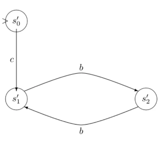
all processes, but not the joint infinite computations of unsynchronized processes. The following example illustrates this situation. Consider the generalized B¨uchi automata A and A′ of Figures 1 and 2 where
F = {{s1}, {s2}} and F′ = {{s′1}, {s′2}} respectively.
A possible trace automaton A∞
T is given in Figure 3.
Its set of sets of accepting states is defined by FT =
{{(s1, s′0), (s1, s′1), (s1, s′2)}, {(s2, s′0)}, {(s1, s′1)},
{(s1, s′2)}}. This automaton does not accept any word
whereas there is a joint infinite execution of the au-tomata A and A′ that would be accepted by the
cor-responding global automaton.
s1 ✖✕ ✗✔ > s2 ✖✕ ✗✔ q a ✐ a
Figure 1: Generalized B¨uchi automaton A
s′ 0 ✖✕ ✗✔ > s′ 1 ✖✕ ✗✔ s′ 2 ✖✕ ✗✔ ❄ c q b ✐ b
Figure 2: Generalized B¨uchi automaton A′
We now formalize the above discussion. Let AG and
A∞
T be respectively the product automaton and the
trace automaton obtained by composing the general-ized B¨uchi automata Ai, 1 ≤ i ≤ n + 1. Consider
a computation of AG or A∞T on an infinite word w.
One can view this computation as an infinite sequence of transitions each of which is an element (s, a, s′) of
s1,s′0 ✖✕ ✗✔ > s2,s′0 ✖✕ ✗✔ q a ✐ a s1,s′1 ✖✕ ✗✔ s1,s′2 ✖✕ ✗✔ ❄ c q b ✐ b
Figure 3: Trace automaton A∞ T
identify the automata Ai that are active (as defined
in Section 3) for this transition. This enables us to define the restriction of a computation of AG or A∞T
to one of the components Ai.
Definition 4.1 Given a trace or product automaton A obtained by composing the generalized B¨uchi au-tomata Ai, 1 ≤ i ≤ n + 1, the restriction of a
compu-tation κ of A to the automaton Ai (denoted κ|Ai) is
the subsequence of κ that contains only the transitions for which Ai is active.
Note that the restriction of a computation of AG or
A∞
T to an automaton Aiis in fact a computation of Ai.
However, the restriction can be finite, even if the the initial computation is infinite. We can nevertheless prove the following.
Theorem 4.1 Let κ be a computation (finite or ω-infinite) of the global automaton AG obtained by
com-posing the automata Ai, 1 ≤ i ≤ n+1. Then, for every
Ai, there is a computation κi (finite or ω-infinite) of
the trace automaton A∞
T such that κ|Ai= κi|Ai.
Note that it is not true that there is a single compu-tation κ′ of A∞
T such that κ|Ai = κ′|Ai for all Ai’s.
In spite of this, Theorem 4.1 lets us obtain an inter-esting result, namely that the trace automaton can be used for model checking in cases where only one of the components is required to have an infinite computa-tion. This is the case if all but one of the automata
Ai have a vacuous accepting condition, i.e. have an
empty set F. We can prove the following.
Theorem 4.2 Let Ai, 1 ≤ i ≤ n + 1 be generalized B¨uchi automata all but one of which have a vacuous accepting condition. Let AG and A∞T be the product
and trace automata obtained by composing the au-tomata Ai. Then, the automaton AG is nonempty
(has at least one infinite accepting computation) iff the trace automaton A∞
T is nonempty.
Theorem 4.2 is obtained from Theorem 4.1 and from the immediate fact that all computations of the trace automaton are also computations of the product au-tomaton. In practice, Theorem 4.2 enables us to use the trace automaton for model checking in the cases where the program does not operate under some fair-ness hypothesis. Indeed, in those circumstances, the automata representing the program will have vacu-ous accepting conditions and the automaton obtained from the formula to be checked will be the only one with a nonempty set F.
5
Automata on (ω × n)-words
Trace automata do not adequately represent the ω-computations of the components from which they are built because infinite computations cannot be concate-nated. Actually, with the help of a little abstraction, infinite computations could very well be concatenated. One can simply think of computations whose length is an ordinal larger than ω. Since we are only interested in the concatenation of a finite number of infinite com-putations we will only study comcom-putations of length ω×n where n ∈ ω. The definitions of Section 2 can be quite naturally extended to words and computations of length ω × n (for other definitions of automata on ordinals, see [9, 8]).
A word of length ω × n over the alphabet Σ is a func-tion w from the ordinal ω × n to Σ. We use automata that are defined exactly as in Section 2 and simply change the definition of a run. A run of an automaton A= (Σ, S, ∆, s0,F) on a word w of length ω × n is a
function σ from ω × n to S that satisfies the following conditions:
1. σ(0) = s0;
2. for each successor ordinal α + 1 ∈ ω × n, (σ(α), w(α), σ(α + 1)) ∈ ∆;
3. for each limit ordinal λ ∈ ω×n, there is an infinite sequence of ordinals α whose limit is λ such that σ(α) = σ(λ).
The notions of accepting run and accepted word are essentially unchanged. A run σ is accepting if, for each Fj ∈ F, there is some state in Fjthat repeats infinitely
often, i.e., for some s ∈ Fj there are infinitely many
i ∈ ω × n such that si = s. The ω × n-word w is
accepted by A if there is an accepting run of A over w. The set of ω × n words accepted by A is denoted Lω×n(A).
Checking that Lω×n(A) is nonempty can be done by
computing the strongly connected components of A. Theorem 5.1 Let A = (Σ, S, ∆, s0,F) be an automa-ton. Then, Lω×n(A) 6= ∅ iff there is a sequence of
strongly connected components C1, . . . Cn in A such
that
• C1 is accessible from s0 and Ci+1 is accessible
from Ci, for 1 ≤ i < n and
• for each Fj∈ F, there is some Ci such that Fj∩
Ci6= ∅.
The interesting aspect of the definitions we have just given is that if we consider the trace automaton as an automaton on words of length ω ×n, then it represents all infinite computations of the combined automata. If we extend the notion of computation used in Section 4 to sequences of transitions of length ω × n, we can prove the following.
Theorem 5.2 Let κ be an ω-computation of the global automaton AG obtained by composing the
au-tomata Ai, 1 ≤ i ≤ n+1. Then, there is a computation
κ′ of length at most ω × (n + 1) of the trace automaton
A∞
T such that for all 1 ≤ i ≤ n + 1, κ|Ai= κ′|Ai.
To use the trace automaton for model checking, we also need the converse of Theorem 5.2. However, this does not hold in general since it requires that a putation of length ω × (n + 1) be merged into a com-putation of length ω. For this to be possible we need to put some restrictions on computations. Consider a computation of length ω×(n+1). For each ω-sequence in this computation, i.e. part of the computation cor-responding to an interval [ω × j, ω × (j + 1)[, we define the repeating part of this ω-sequence as its suffix that only contains states that appear infinitely often. The rest of the ω-sequence is then its finite prefix. We call a computation separable if for all 0 ≤ i < j ≤ n, all transitions in the repeating part of [ω × i, ω × (i + 1)[ are independent of all transitions in the finite prefix of [ω ×j, ω ×(j +1)[. We can then show that the converse of Theorem 5.2 holds for separable computations and hence the following.
Theorem 5.3 Let Ai, 1 ≤ i ≤ n + 1 be generalized B¨uchi automata. Let AG and A∞T be the product and
trace automata obtained by composing the automata Ai. Then, the automaton AGis nonempty (has at least
one accepting computation) iff the trace automaton A∞
T has at least one separable computation of length
at most ω × (n + 1).
Furthermore, note that Theorem 5.1 can be adapted to separable computations by requiring that for all 1 ≤ i < j ≤ (n + 1), the transitions appearing in Ci are independent from those appearing in the path
from Cj−1 to Cj. Combining this observation with
Theorem 5.3 we have a criterion for solving the model-checking problem in terms of the trace automaton A∞
T .
6
Conclusions and Comparison with
Other Work
The closest work to the one presented here is certainly that of Valmari [40]. However, while it has the same goal it does not achieve the same results. Indeed, Val-mari only handles a temporal logic where the opera-tor “next” cannot appear. We handle the full logic and, actually, we can also handle extended temporal logics like that of [45]. Also, in [40] concurrency is modelled by interleaving for all actions that appear in the formula. Because in our method the automa-ton for the formula is combined with the program, we do not have this drawback. Moreover, to solve the problem that trace automata do not adequately represent the infinite behaviors of a set of processes, Valmari has to modify the construction of the automa-ton and actually build an automaautoma-ton that will usually have more states and transitions. We solve this prob-lem by viewing the trace automaton as an automaton on ω × n-words. Finally, the possibility of modelling fairness conditions within the program is not present in [40]. All the advantages above are linked to the strategy we use for solving the model-checking prob-lem which, as we have shown, is quite distinct from Valmari’s. However, at the heart of both methods lies an algorithm for computing an automaton that only represents “some” interleavings of concurrent events: Valmari uses an algorithm based on “Stubborn Sets”, we use the construction of the “Trace Automaton” given in [22]. This algorithm also influences the effec-tiveness of a model-checking method. Unfortunately, this influence is not at all as clear cut as that of the strategy. It is quite possible that for some problems the “Trace Automaton” algorithm is best whereas for others the “Stubborn Sets” one is preferable.
a precise answer since it might be no better than in-terleaving methods when there is very tight coupling between the processes and dramatically better when there is no coupling between the processes. In the latter case, we could claim as is done in [10] that we can check systems with astronomical numbers of (in-terleaving semantics) states. Of course this is rather meaningless since the trick is not to explore all states either by treating classes of states as one state (the ap-proach of [10]) or by completely avoiding parts of the state space (our approach). The only real fact we can give is that experimental results with trace automata are very encouraging.
Finally, note that our method has the advantages of “on the fly verification” [16, 26, 4, 24]. By this we mean, that we build the automaton for the combina-tion of the program and property without ever build-ing the automaton for the program. Maybe surpris-ingly, this automaton is often smaller than the au-tomaton for the program alone because the property acts as a constraint on the behavior of the program. Our method thus has a head start over methods that require the state graph of the program to be built.
Acknowledgements
We wish to thank David Dill, Antti Valmari and anonymous referees for helpful comments on this pa-per.
References
[1] Alfred V. Aho, John E. Hopcroft, and Jeffrey D. Ullman. The Design and Analysis of Computer Algorithms. Addison Wesley, Reading, 1974. [2] R. Alur, C. Courcoubetis, and D. Dill.
Model-checking for real-time systems. In Proceedings of the 5th Symposium on Logic in Computer Sci-ence, pages 414–425, Philadelphia, June 1990. [3] R. Alur and T. Henzinger. Real-time logics:
com-plexity and expressiveness. In Proceedings of the 5th Symposium on Logic in Computer Science, Philadelphia, June 1990.
[4] A. Bouajjani, J. C. Fernandez, and N. Halbwachs. On the verification of safety properties. Technical Report SPECTRE L12, IMAG, Grenoble, march 1990.
[5] M. Browne, E.M. Clarke, and D.L. Dill. Au-tomatic circuit verification using temporal logic: Two new examples. In IEEE Int. Conf. on Computer Design: VLSI and Computers, Port Chester, October 1985.
[6] Michael C. Browne. An improved algorithm for the automatic verification of finite state systems using temporal logic. In Proceedings of the First Symposium on Logic in Computer Science, pages 260–266, Cambridge, June 1986.
[7] J.R. B¨uchi. On a decision method in restricted second order arithmetic. In Proc. Internat. Congr. Logic, Method and Philos. Sci. 1960, pages 1–12, Stanford, 1962. Stanford University Press.
[8] J.R. B¨uchi. Decision methods in the theory of ordinals. Bull of the AMS, 71:767–770, 1965. [9] J.R. B¨uchi. Transfinite automata recursions and
weak second order theory of ordinals. In Proc. Internat. Congr. Logic, Method and Philos. Sci. 1964, pages 2–23, Amsterdam, 1965. North Hol-land.
[10] J.R. Burch, E.M. Clarke, K.L. McMillan, D.L. Dill, and L.J. Hwang. Symbolic model checking: 1020 states and beyond. In Proceedings of the
5th Symposium on Logic in Computer Science, Philadelphia, June 1990.
[11] E. M. Clarke and O. Gr¨umberg. Avoiding the state explosion problem in temporal logic model-checking algorithms. In Proc. 6th ACM Sym-posium on Principles of Distributed Computing, pages 294–303, Vancouver, British Columbia, Au-gust 1987.
[12] E. M. Clarke, O. Gr¨umberg, and M. C. Browne. Reasoning about networks with many identical finite-state processes. In Proc. 5th ACM Sym-posium on Principles of Distributed Computing, pages 240–248, Calgary, Alberta, August 1986. [13] E.M. Clarke, E.A. Emerson, and A.P. Sistla.
Au-tomatic verification of finite-state concurrent sys-tems using temporal logic specifications. ACM Transactions on Programming Languages and Systems, 8(2):244–263, January 1986.
[14] R. Cleaveland. Tableau-based model checking in the propositional mu-calculus. Acta Informatica, 27:725–747, 1990.
[15] O. Coudert, J. C. Madre, and C. Berthet. Veri-fying temporal properties of sequential machines without building their state diagram. In Proc. Workshop on Computer Aided Verification, Rut-gers, June 1990.
[16] C. Courcoubetis, M. Vardi, P. Wolper, and M. Yannakakis. Memory efficient algorithms for the verification of temporal properties. In Proc. Workshop on Computer Aided Verification, Rut-gers, June 1990.
[17] C. Courcoubetis and M. Yannakakis. Markov de-cision processes and regular events. In Proc. 17th Int. Coll. on Automata Languages and Program-ming, volume 443, Coventry, July 1990. Lecture Notes in Computer Science, Springer-Verlag. [18] E.A. Emerson and C.-L. Lei. Modalities for model
checking: Branching time logic strikes back. In Proceedings of the Twelfth ACM Symposium on Principles of Programming Languages, pages 84– 96, New Orleans, January 1985.
[19] E.A. Emerson and C.-L. Lei. Temporal model checking under generalized fairness constraints. In Proc. 18th Hawaii International Conference on System Sciences, Hawaii, 1985.
[20] E.A. Emerson and C.-L. Lei. Modalities for model checking: Branching time logic strikes back. In Proceedings of the First Symposium on Logic in Computer Science, pages 267–278, Cambridge, June 1986.
[21] S. German and A.P. Sistla. Reasoning with many processes. In Proc. Symp. on Logic in Computer Science, pages 138–152, Ithaca, June 1987. [22] P. Godefroid. Using partial orders to improve
au-tomatic verification methods. In Proc. Workshop on Computer Aided Verification, Rutgers, June 1990.
[23] S. Graf and B. Steffen. Using interface specifica-tions for compositional reduction. In Proc. Work-shop on Computer Aided Verification, Rutgers, June 1990.
[24] N. Halbwachs, D. Pilaud, F. Ouabdesselam, and A.C. Glory. Specifying, programming and verify-ing real-time systems, usverify-ing a synchronous declar-ative language. In Workshop on automatic ver-ification methods for finite state systems, LNCS 407. Springer Verlag, june 1989.
[25] E. Harel, O. Lichtenstein, and A. Pnueli. Explicit-clock temporal logic. In Proceedings of the 5th Symposium on Logic in Computer Science, pages 402–413, Philadelphia, June 1990.
[26] C. Jard and T. Jeron. On-line model-checking for finite linear temporal logic specifications. In Automatic Verification Methods for Finite State Systems, Proc. Int. Workshop, Grenoble, volume 407, pages 189–196, Grenoble, June 1989. Lecture Notes in Computer Science, Springer-Verlag. [27] Y. Kornatzky and S. S. Pinter. A model checker
for partial order temporal logic. EE PUB 597, Department of Electrical Enginering, Technion-Israel Institute of Technology, 1986.
[28] R. P. Kurshan and K. McMillan. A structural in-duction theorem for processes. In Proceedings of the Eigth ACM Symposium on Principles of Dis-tributed Computing, Edmonton, Alberta, August 1989.
[29] O. Lichtenstein and A. Pnueli. Checking that fi-nite state concurrent programs satisfy their lin-ear specification. In Proceedings of the Twelfth ACM Symposium on Principles of Programming Languages, pages 97–107, New Orleans, January 1985.
[30] A. Mazurkiewicz. Trace theory. In Petri Nets: Applications and Relationships to Other Models of Concurrency, Advances in Petri Nets 1986, Part II; Proceedings of an Advanced Course, vol-ume 255 of Lecture Notes in Computer Science, pages 279–324, 1986.
[31] W. Penczek. Proving partial order properties us-ing cctl. Submitted to Proc. Concurrency and Compositionality Workshop, San Miniato, Italy, 1990.
[32] S. Pinter and P. Wolper. A temporal logic for reasoning about partially ordered computations. In Proc. 3rd ACM Symposium on Principles of Distributed Computing, pages 28–37, Vancouver, August 1984.
[33] A. Pnueli and L. Zuck. Probabilistic verification by tableaux. In Proc. 1st Symp. on Logic in Com-puter Science, pages 322–331, Cambridge, June 1986.
[34] D. K. Probst and H. F. Li. Using partial-order semantics to avoid the state explosion problem in asynchronous systems. In Proc. Workshop on Computer Aided Verification, Rutgers, June 1990.
[35] J.P. Quielle and J. Sifakis. Specification and ver-ification of concurrent systems in cesar. In Proc.
5th Int’l Symp. on Programming, volume 137, pages 337–351. Springer-Verlag, Lecture Notes in Computer Science, 1981.
[36] J.L. Richier, C. Rodriguez, J. Sifakis, and J. Vo-iron. Verification in xesar of the sliding window protocol. In Proc. IFIP WG 6.1 7th Int. Conf. on Protocol Specification, Testing and Verification, pages 235–250, Zurich, 1987. North Holland. [37] C. Stirling and D. Walker. Local model checking
in the modal mu-calculus. In Proc. 15th Col. on Trees in Algebra and Programming. Lecture Notes in Computer Science, Springer-Verlag, 1989. [38] Andr´e Thayse and et al. From Modal Logic to
Deductive Databases: Introducing a Logic Based Approach to Artificial Intelligence. Wiley, 1989. [39] A. Valmari. Stubborn sets for reduced state space
generation. In Proc. 10th International Confer-ence on Application and Theory of Petri Nets, volume 2, pages 1–22, Bonn, 1989.
[40] A. Valmari. A stubborn attack on state explosion. In Proc. Workshop on Computer Aided Verifica-tion, Rutgers, June 1990.
[41] M. Vardi. Automatic verification of probabilistic concurrent finite-state programs. In Proc. 26th IEEE Symp. on Foundations of Computer Sci-ence, pages 327–338, Portland, October 1985. [42] M. Vardi. A temporal fixpoint calculus. In Proc.
15th ACM Symp. on Principles of Programming Languages, pages 250–259, San Diego, January 1988.
[43] M. Vardi. Unified verification theory. In B. Ban-ieqbal, H. Barringer, and A. Pnueli, editors, Proc. Temporal Logic in Specification, volume 398, pages 202–212. Lecture Notes in Computer Science, Springer-Verlag, 1989.
[44] M.Y. Vardi and P. Wolper. An automata-theoretic approach to automatic program verifi-cation. In Proc. Symp. on Logic in Computer Science, pages 322–331, Cambridge, june 1986. [45] P. Wolper. Temporal logic can be more
expres-sive. Information and Control, 56(1–2):72–99, 1983.
[46] P. Wolper. On the relation of programs and computations to models of temporal logic. In
B. Banieqbal, H. Barringer, and A. Pnueli, ed-itors, Proc. Temporal Logic in Specification, vol-ume 398, pages 75–123. Lecture Notes in Com-puter Science, Springer-Verlag, 1989.
[47] P. Wolper and V. Lovinfosse. Verifying prop-erties of large sets of processes with network invariants. In Automatic Verification Methods for Finite State Systems, Proc. Int. Workshop, Grenoble, volume 407, pages 68–80, Grenoble, June 1989. Lecture Notes in Computer Science, Springer-Verlag.
[48] P. Wolper, M.Y. Vardi, and A.P. Sistla. Reason-ing about infinite computation paths. In Proc. 24th IEEE Symposium on Foundations of Com-puter Science, pages 185–194, Tucson, 1983.