arXiv:1906.00762v1 [astro-ph.SR] 3 Jun 2019
Astronomy & Astrophysicsmanuscript no. 35141final c ESO 2019
June 4, 2019
Variations on a theme – the puzzling behaviour of Schulte 12
⋆
Ya¨el Naz´e
1⋆⋆, Gregor Rauw
1, Stefan Czesla
2, Laurent Mahy
3, and Fran Campos
41 Groupe d’Astrophysique des Hautes Energies, STAR, Universit´e de Li`ege, Quartier Agora (B5c, Institut d’Astrophysique et de
G´eophysique), All´ee du 6 Aoˆut 19c, B-4000 Sart Tilman, Li`ege, Belgium e-mail: [email protected]
2 Hamburger Sternwarte, Universit¨at Hamburg, Gojenbergsweg 112, 21029, Hamburg, Germany 3 Instituut voor Sterrenkunde, KU Leuven, Celestijnlaan 200D, Postbus 2401, 3001, Leuven, Belgium 4 Observatori Puig dAgulles, Passatge Bosc 1, 08759 Vallirana, Barcelona, Spain
Preprint online version: June 4, 2019
ABSTRACT
One of the first massive stars detected in X-rays, Schulte 12 has remained a puzzle in several aspects. In particular, its extreme brightness both in the visible and X-ray ranges is intriguing. Thanks to Swift and XMM-Newton observations covering ∼5000 d, we report the discovery of a regular 108 d modulation in X-ray flux of unknown origin. The minimum in the high-energy flux appears due to a combination of increased absorption and decreased intrinsic emission. We examined in parallel the data from a dedicated spectroscopic and photometric monitoring in the visible and near-IR domains, complemented by archives. While a similar variation timescale is found in those data, they do not exhibit the strict regular clock found at high energies. Changes in line profiles cannot be related to binarity but rather correspond to non-radial pulsations. Considering the substantial revision of the distance of Schulte 12 from the second GAIA data release, the presence of such oscillations agrees well with the evolutionary status of Schulte 12, as it lies in an instability region of the HR diagram.
Key words.stars: early-type – stars: massive – stars: winds – X-rays: stars – supergiants – stars: variable: general – stars: individual:
Schulte 12
1. Introduction
In 1978, the Einstein observatory detected for the first time X-rays associated to massive stars (Harnden et al., 1979; Ku & Chanan, 1979; Seward et al., 1979). Among these was Cyg OB2 #12 or Schulte 12 (V=12.5), a highly reddened and peculiar star known for several decades (Morgan et al., 1954). Schulte 12 was classified as an early B hypergiant of spec-tral type B3–4Ia+ (Clark et al., 2012). With its extreme bright-ness, the star would be placed in the Hertzprung-Russell dia-gram above the Humphreys-Davidson limit. This explains why Schulte 12 was often considered as a luminous blue variable (LBV) candidate (Clark et al., 2005). In support of this classifi-cation, evidence for changes in spectral type (B3–B8) have been presented by Massey & Thompson (1991) and Kiminki et al. (2007). Variations of the temperature were later refuted by Clark et al. (2012) because of the low signal-to-noise ratio of the data, prohibiting changes to reach a low significance level, but also because changes in apparent spectral type may not necessarily reflect a varying photosphere hence could agree with a constant temperature. A lack of helium enrichment is also at odds with an evolved star status (Clark et al., 2012). ⋆ Based on X-ray observations collected with ASCA, Suzaku,
Chandra and especially Swift and XMM-Newton, an ESA Science Mission with instruments and contributions directly funded by ESA Member States and the USA (NASA). Optical photometry from NSVS, Integral-OMC, and ASAS-SN are also used, as well as optical spec-troscopy from the Hermes and Carmenes instruments. Hermes is in-stalled on the Mercator Telescope, which is operated on the island of La Palma by the Flemish Community, at the Spanish Observatorio del Roque de los Muchachos of the Instituto de Astrof´ısica de Canarias.
⋆⋆ F.R.S.-FNRS Research Associate.
Furthermore, no surrounding ejected nebulosities seem to exist (Kobulnicky et al., 2012; Oskinova et al., 2017).
The early X-ray detection poses a puzzle which could not be solved in the four decades elapsed since then. Indeed, the X-ray emission of Schulte 12 is bright (log[LX/LBOL] =
−6.1) and presents a hard (kT ∼ 2 keV) component (Rauw, 2011). This is clearly at odds with the properties of LBVs, which generally present very faint (undetected) X-ray emissions (Naz´e et al., 2012a). Besides, it is also at odds with typical prop-erties of massive stars. The intrinsic X-rays from massive stars with fast winds (thousands of km s−1) are generally thought
to come from embedded wind shocks (e.g. Feldmeier et al., 1997), which generate soft (kT = 0.3 − 0.6 keV) and mod-estly bright (log[LX/LBOL] ∼ −7 for O-stars) X-ray
emis-sions (Oskinova, 2005; Naz´e, 2009; Rauw et al., 2015a). In this context, it is interesting to note that Schulte 12 actually has a very slow wind (v∞ = 400 km s−1, Clark et al. 2012 or even
150 km s−1, Klochkova & Chentsov 2004), incompatible with
high-temperature plasma - though larger velocities have also been proposed; see Leitherer et al. (1982).
There is however another Galactic LBV that displays bright and hard X-rays: η Carinae. In this case, they arise from the face-on collisiface-on between the two winds of the compface-onents in this massive binary (see e.g. Hamaguchi et al., 2014, and references therein). Similarly, the LBV HD 5980 in the Small Magellanic Cloud also emits bright and hard X-rays linked to a wind–wind collision (Naz´e et al., 2018b, and references therein). A telltale signature of such colliding winds is variability (for a review, see Rauw & Naz´e, 2016). Indeed, the intrinsic strength of the col-lision changes with the stellar separation in eccentric binaries and the absorption may also vary as the shocked plasma is
al-ternately seen through the two different winds (Stevens et al., 1992). Because they are linked to the orbital configuration, such changes recur with the orbital period. For Schulte 12, variations of its X-ray emission have been reported several times (Rauw, 2011; Yoshida et al., 2011; Cazorla et al., 2014) but no periodic-ity was found. In view of the apparently monotonic decrease in X-ray fluxes from 2004 to 2013, an alternative scenario where X-rays are produced by fading shocks between slow-moving ejecta and fast winds after an eruption could not be rejected (Cazorla et al., 2014).
The possible presence of a companion to Schulte 12 has been considered in the past (Souza & Lutz, 1980) and has subsequently been revived in a few recent studies. First, Caballero-Nieves et al. (2014) reported the detection of a close visual companion at 64 mas with ∆V = 2.3. Maryeva et al. (2016) confirmed its presence and constrained its orbital period to 100–200 yrs from its slight change of position. These latter au-thors also found a third object further out at 1.2′′with ∆m = 4.8.
However, such distant companions are unlikely to produce an X-ray bright wind–wind collision as plasma density would be too small at such large separations. Until now, X-ray bright wind– wind collisions have been found in massive binaries with peri-ods of a few years (up to a decade in 9 Sgr; Rauw et al. 2016), not decades or centuries. Secondly, small line-profile and radial-velocity (RV) changes were reported by Klochkova & Chentsov (2004) and Chentsov et al. (2013) but they could not confirm or rule out the binarity hypothesis (Chentsov et al., 2013). Only a double-lined spectroscopic binary seemed excluded by the data (see also Clark et al., 2012). Finally, Oskinova et al. (2017) stud-ied a high-resolution X-ray spectrum of Schulte 12 and found rather strong f lines in f ir triplets from He-like ions. While the Si xiii triplet is compatible with the absence of depopulation of the upper level of the f line, the Mg xi lines suggest some depop-ulation, though not due to UV radiation but to collisions: there would thus be dense plasma where X-rays arise. This could be compatible with X-ray generation very close to the photosphere or in a wind–wind collision. The latter scenario is further sup-ported by the (broad and unshifted) profiles of X-ray lines and the lack of very strong absorption. Oskinova et al. (2017) fur-ther suggested a late-O type for the optically closest companion, if there was a wind–wind interaction between this star and the LBV (which remains to be demonstrated). However, they inter-preted the observed X-ray variability as being random and in-compatible with a companion on a long (decades) orbit.
While important information has been gained in recent years, the nature of Schulte 12 is still not fully understood. Time is thus ripe to perform an in-depth study, with a thorough X-ray and op-tical monitoring (described in Section 2). The derived results led to several surprises (Sections 3 and 4 for X-ray and optical/near-IR findings, respectively). Their possible interpretation is dis-cussed in Section 5 and then summarized in Section 6.
2. Observations and data reduction
2.1. Optical and near-IR domains 2.1.1. Photometry
Photometry of Schulte 12 was obtained in both the Ic and V fil-ters at the private observatory of one of the current authors (F.C.), situated in Vallirana (near Barcelona, Spain) and equipped with a Newton telescope of 20cm diameter (with f/4.7 and a German equatorial mount). The camera is a CCD SBIG ST-8XME (KAF 1603ME). The exposures were typically of 180 s and 120 s du-ration for the V and Ic filters, respectively.
Table 1.Journal of the optical and near-IR spectroscopic obser-vations. HJD correspond to dates at mid-exposure and S/Ns are evaluated at 7525Å. Hermes Carmenes Date HJD S NR Date HJD S NR YYMMDD –2 450 000 YYMMDD –2 450 000 20100626 5373.640 240 20170524 7898.611 250 20110709 5751.665 260 20170607 7912.647 310 20110828 5801.572 170 20170623 7928.628 290 20110903 5807.605 220 20180502 8241.666 160 20121115 6247.331 210 20180512 8251.647 50 20131106 6603.394 200 20180525 8264.632 180 20140606 6814.652 220 20180530 8269.608 250 20150710 7213.631 220 20180614 8284.568 290 20151128 7355.350 60 20180620 8290.648 250 20160623 7562.663 170 20180625 8295.573 280 20160708 7578.467 140 20180630 8300.544 200 20170529 7902.611 240 20180714 8314.553 80 20180721 8321.585 180 20180804 8335.484 250 20180811 8342.572 250 20180817 8348.455 310 20180825 8356.455 240 20180904 8366.396 210 20180913 8375.367 110
The images were corrected for bias, dark current, and flat-field in the usual way using the data-reduction software Maxim DL v51. The photometry was extracted with the FotoDif v3.93
software, using as comparison star SAO 49783 (TYC 3157-195-1). Four stars (TYC 3157-1310-1, TYC 3157-603-1, TYC 3161-1269-1, TYC 3157-463-1) were further measured to check the stability of the solution.
2.1.2. Spectroscopy
Schulte 12 was observed 12 times between 2010 and 2017 with the Hermes spectrograph (Raskin et al., 2011) installed on the 1.2 m Mercator telescope on La Palma (Spain). Given the mag-nitude of the star, between 2 and 7 consecutive exposures of 1800 s (depending on the weather conditions) were summed up to increase S/N. The data were taken in the high-resolution fibre mode, which has a resolving power of R ∼ 85000. The spectra cover the 4000–9000Å wavelength domain but because of the high extinction of the star, the range below 5750Å was not used for the present analysis. The raw exposures were reduced using the dedicated Hermes pipeline and we worked with the extracted cosmic-removed, merged spectra afterwards.
A set of 19 observations were obtained with the Carmenes (Calar Alto high-Resolution search for M dwarfs with Exoearths with near-IR and optical Echelle Spectrographs; Quirrenbach et al., 2018) instrument at the 3.5 m telescope of the Centro Astron´omico Hispano Alem´an at Calar Alto Observatory (Spain). These observations were granted via the OPTICON common time allocation process (program IDs 2018A/004 and 2018B/001) and through German open time (program ID F17-3.5-002). Carmenes features a dichroic that shares the light be-tween two separate echelle spectrographs: the first one covering the optical domain from about 5200 to 9600 Å at a spectral re-solving power near R = 94 600, and the second covering the near-IR from about 9600 Å to 1.71 µm at R = 80 400. All data
were obtained in service mode at a rate of about one observa-tion every 10 d during our main observing campaign in May– August 2018, and the exposure times were 4 × 5 min per observ-ing night. The data were reduced usobserv-ing the Carmenes pipeline (Caballero et al., 2016). The Carmenes spectra taken the same night were combined to improve S/Ns.
Table 1 lists the dates of these spectra, as well as their S/Ns around 7525Å. Because of the strong extinction, typical S/Ns vary from ∼50 at 5800Å to ∼300 in the near-IR. To obtain the best diagnostics, we focused on wavelength intervals with strong stellar lines and limited contamination by interstellar or telluric lines. However, small contamination could not always be totally avoided. We therefore performed a correction for telluric lines around Hα, He i λ 7065Å, and He i λ 10830Å, as well as Paschen lines at 8500–8900Å and 1µm. This was done within IRAF using the telluric template of Hinkle et al. (2000) in the optical range and a telluric spectrum calculated for Calar Alto with molecfit (Smette et al., 2015) in the near-IR. As a last step, the spectra were normalized over limited wavelength windows using splines of low order.
2.2. X-ray domain
2.2.1.XMM-Newton
The Li`ege group have obtained ten observations of the Cyg OB2 region since the launch of XMM-Newton. The oldest ones were reported in De Becker et al. (2006), Rauw (2011), Naz´e et al. (2012b), and Cazorla et al. (2014). Schulte 12 also appears in six additional XMM-Newton exposures centred on PSR J2032+4127. However, in these exposures it is far off-axis and only in the field-of-view of the MOS2 detectors. Moreover, stray light from Cyg X-3 contaminates the source (further discussed below). All datasets were reduced with SAS v16.0.0 using cali-bration files available in Fall 2017 and following the recommen-dations of the XMM-Newton team2. No barycentric correction
was applied to event arrival times.
The EPIC observations were taken in the full-frame mode and with the medium filter (to reject optical/UV light), except for ObsID 0677980601 where the large window mode was used for the MOS cameras to avoid pile-up in Cyg OB2 #9 (which was then at its maximum). After pipeline processing, the data were filtered to keep only best-quality data (pattern of 0–12 for MOS and 0–4 for pn). Background flares were detected in sev-eral observations (Revs 0896, 0911, 1353, 1355, 2114, 3097). Only times with a count rate above 10. keV lower than 0.2– 0.3 cts s−1(for MOS) or 0.4 cts s−1(for pn) were kept. A source
detection was performed on each EPIC dataset using the task
edetect chainon the 0.3–2.0 keV (soft) and 2.0–10.0 keV (hard)
energy bands and for a minimum log-likelihood of 10. This task searches for sources using a sliding box and determines the fi-nal source parameters from point spread function (PSF) fitting; the final count rates correspond to equivalent on-axis, full-PSF count rates (Table A.1). It may be noted in this table that the count rates of Schulte 12 in the off-axis observations are unreli-able, as demonstrated by their much larger hardness ratios (due to uncorrected contamination by stray light).
We then extracted EPIC spectra of Schulte 12 using the task especget in circular regions of 35′′ radius (to avoid
nearby sources) centred on the Hipparcos positions (reported in Simbad). For ObsID 0793183001, the source appears so far
off-2 SAS threads, see
http://xmm.esac.esa.int/sas/current/documentation/threads/
axis that a larger ellipse was needed to extract it. On the contrary, in a few other cases the extraction radius had to be reduced for one of the EPIC cameras to avoid nearby CCD gaps. Whenever the core of the source fell in one such gap, the spectrum was not extracted to avoid large uncertainties. For the background, a circular region of 35′′ radius was chosen in a region devoid of
sources and as close as possible to the target. Dedicated ARF and RMF response files, which are used to calibrate the flux and energy axes, respectively, were also calculated by this task. EPIC spectra were grouped, with specgroup, to obtain an over-sampling factor of five and to ensure that a minimum S/N of 3 (i.e. a minimum of 10 counts) was reached in each spectral bin of the background-corrected spectra.
2.2.2.Swift
At our request, the Cyg OB2 region was observed 18 times by the Neil Gehrels Swift Observatory. In addition, the same area was the subject of a short campaign in June–July 2015 and it serendipitously appears from time to time in the field of view of observations dedicated to PSR J2032+4127 (Petropoulou et al., 2018), 3EGJ2033+4118, or WR 144. All these XRT data taken in Photon Counting mode were retrieved from the HEASARC archive centre and were further processed locally using the XRT pipeline of HEASOFT v6.22.1 with calibrations v20170501. Because of the high extinction towards Cyg OB2, no optical loading is expected for XRT data of Schulte 12. The source spec-tra were exspec-tracted within Xselect using a circular region of 35′′
radius; a nearby region devoid of any source was used for the background. The spectra were binned using grppha in a similar manner as the XMM-Newton spectra. The adequate RMF matrix from the calibration database was used whilst specific ARF re-sponse matrices were calculated for each dataset using xrtmkarf, considering the associated exposure map. Corrected count rates in the same energy bands as XMM-Newton were obtained for each observation from the UK online tool3, and they are reported
in Table A.1.
UVOTphotometry was taken in parallel with the X-ray data
using a variety of filters. Following the recommendations of the
Swiftteam4, magnitudes were extracted from Level2 files using
an extraction region of 5′′ radius for the source (and the same
coordinates as in X-rays) while a nearby region of 15′′ radius
and devoid of sources was used as background. The resulting photometry is provided in the last column of Table A.1, where the reported errors correspond to the combination of systematic and statistical errors. No significant correlation is found between X-ray count rates and UV photometry.
2.2.3.Chandra
The massive stars of Cyg OB2 are X-ray bright, and there-fore suffer from pile-up in usual Chandra-ACIS observations. However, Schulte 12 was also observed twice with Chandra-HETG (Table A.1). We reprocessed these data using CIAO 4.9 and CALDB 4.7.3. In the first dataset (ObsID=2572), Schulte 12 appears far off-axis: its high-resolution spectrum is of low qual-ity (Oskinova et al., 2017), but this position, leading to a larger PSF, allows its order spectrum to avoid pile-up. This zero-order spectrum was therefore extracted using specextract in a circle of radius 20 px (9.8′′) centred on the Simbad coordinates
of the star and a nearby circle of 14.8′′ radius was used as
3 http://www.swift.ac.uk/user objects/
background region. The second exposure (ObsID=16659) was pointed at Schulte 12, and therefore the high-resolution HEG and MEG spectra were extracted, combining the orders +1 and –1 for each grating, in addition to the zeroth-order spectrum. Specific detector response matrices (RMF and ARF) were calculated to obtain energy- and flux-calibrated spectra and a grouping similar to that used for XMM-Newton spectra was applied.
2.2.4. JAXA facilities
ASCAobserved Cyg OB2 in April 1993 while Suzaku did so in
December 2007. We downloaded these archival data from the HEASARC website and reduced them according to recommen-dations5.
The ASCA observation of Cyg OB2 consists of several datasets because of two different data modes (BRIGHT and BRIGHT2) and bit rates (high and medium). In all of them, Schulte 12 appears in the middle of stray light due to Cyg X-3. We extracted in Xselect the individual SIS-0 and SIS-1 spec-tra using a circle of 80′′ radius, to avoid the emissions of the
neighbouring stars, and considering the background from the surrounding annulus (with an external radius of 199′′) to best
compensate the stray light contamination. Data from high and medium bit rates were combined, but those from the two modes and two detectors were extracted separately, leading to four spectra in total. Following recommendations, RMF and ARF re-sponses were calculated using the task sisrmg (for grades 0234) and the task ascaarf (for a point source and simple case), respec-tively. A grouping similar to that used for XMM-Newton spectra was applied with grppha. However, the final spectra were found to be extremely noisy and therefore unusable, so they were dis-carded from our analysis.
In Suzaku observations, we extracted in Xselect the individ-ual XIS-0, XIS-1, and XIS-3 spectra of Schulte 12 in a circle of 80′′ radius, to avoid the neighbouring emissions, and we used
a nearby circle of 100′′ radius for the background. Response
files were automatically calculated in Xselect using the calibra-tion database of June 2016. A grouping similar to that used for XMM-Newton spectra was applied with grppha.
3. X-ray results
3.1. Light curves
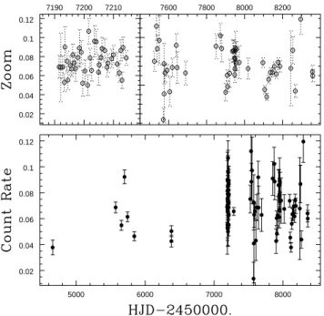
As found previously with XMM-Newton (Cazorla et al., 2014), the Swift light curve in the total band clearly displays varia-tions of a large amplitude, with rates appearing mostly between 0.04 and 0.10 cts s−1 (Fig. 1). These changes do not appear
cor-related to hardness changes. To better characterise these vari-ations in X-ray brightness, we applied a set of period-search algorithms: (1) the Fourier algorithm adapted to sparse/uneven datasets (Heck et al., 1985; Gosset et al., 2001, see also its re-cent rediscovery by Zechmeister & K¨urster 2009 - these pa-pers also note that the method of Scargle 1982, while popu-lar, is not fully statistically correct), (2) three binned analy-ses of variances (Whittaker & Robinson 1944, Jurkevich 1971 which is identical, with no bin overlap, to the “pdm” method of Stellingwerf 1978, and Cuypers 1987 - which is identical to the “AOV” method of Schwarzenberg-Czerny 1989), (3) con-ditional entropy (Cincotta et al., 1999; Cincotta, 1999, see also Graham et al. 2013), and (4) two different string length
meth-5 See cookbooks on https://heasarc.gsfc.nasa.gov/docs/asca/abc/abc.html
and http://heasarc.gsfc.nasa.gov/docs/suzaku/analysis/abc/ 5000 6000 7000 8000 0.02 0.04 0.06 0.08 0.1 0.12 7190 7200 7210 0.02 0.04 0.06 0.08 0.1 0.12 7600 7800 8000 8200
Fig. 1. Swiftlight curve of Schulte 12.
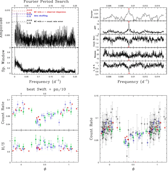
ods (Lafler & Kinman, 1965; Renson, 1978). The Fourier pe-riodogram (top left panel of Fig. 2) clearly reveals a peak at
P =108.11 ± 0.32 d - the error here corresponds to the accuracy
with which the period can be determined (i.e. a small fraction of the peak width). As expected from the spectral window (bot-tom part of the top left panel of Fig. 2), the peak is accompanied by secondary peaks, which are aliases of the main one and are not discussed further. The periodicity is confirmed by the other methods (that find P in the range 107.99–109.05d), even though some of them, especially the string length methods, are less sen-sitive. If we divide the XMM-Newton EPIC-pn count rates by a factor of ten and make a period search on all XMM-Newton and
Swift data combined, then a period of P = 107.99 ± 0.23 d is
found by the Fourier method, with P = 107.64 − 108.45d for the others (top right panel of Fig. 2).
The significance of this X-ray period can be readily esti-mated for the AOV method using the F statistics. The ampli-tude in the AOV periodogram corresponds to the ratio of the variance of the individual means in M phase bins and the sum over all phase bins of the variances about the mean within each bin. Amplitude therefore follows an F-distribution with (M − 1, N − M) degrees of freedom, with M the number of bins (chosen equal to 10) and N the number of data points (e.g. N=96 for Swift data and 106 for Swift+XMM-Newton data). For the top-right AOV panel of Fig. 2, significance levels of <0.01% are formally reached for amplitudes above 4.3.: the observed peak amplitude therefore corresponds to a significance level well be-low 0.01%.
For the Fourier method, no analytical formula can be used to determine the significance level of the highest peak in case of uneven sampling, but the significance level can be estimated in other ways. First, we performed two sets of 10 000 Monte-Carlo simulations considering the observation times and draw-ing at random the individual count rates from a Gaussian dis-tribution with the same mean for all simulations and a standard deviation equal to (1) the observational error on the count rate at each time or (2) the dispersion of the observed count rates. The
0 0.05 0.1 0.15 0.2 0.25 0 0.005 0.01 0.015 0 0.05 0.1 0.15 0.2 0.25 0 0.2 0.4 0.6 0.8 0.006 0.008 0.01 0.012 0.014 0 0.005 0.01 0.015 0 5 10 1.3 1.4 1.5 1.6 10 20 30 0.006 0.008 0.01 0.012 0.014 0.4 0.6 0.8 1 1.2 0 0.5 1 0.04 0.06 0.08 0.1 0 0.5 1 0 0.5 1 0 0.5 1 0 0.05 0.1 0.15
Fig. 2. Top left:Fourier periodogram calculated from the Swift light curve, showing a clear peak at low frequencies. Significance levels of 0.1% and 0.01%, derived from tests (see text for details), are shown as dotted and dashed lines, respectively. Top right: Comparison of period search results on the light curve composed of Swift data and scaled EPIC-pn data with different methods: the same peak (maxima for Fourier and AOV, minima for Renson, Lafler & Kinman, and conditional entropy) is detected in all cases and marked by a star. Bottom left: Phase-folded X-ray light curve, using P = 107.99 d and T0=2 458 288.654. Our 2018 Swift
monitoring campaign of Schulte 12 is shown in green and other high-quality (error on count rate < 0.008 cts s−1) Swift points in
blue; EPIC-pn count rates divided by ten are shown as red stars; we note the good agreement between all data. Bottom right: Same as previous, but with the lower-quality Swift data shown in dotted black.
first test probes the existence of the periodicity against a con-stant signal considering only the observational errors, while the second one tries to reproduce the variability range of the data assuming random variations, thereby testing a different null hy-pothesis. Secondly, we performed another test by shuffling the data 10 000 times: the count rate values were randomly associ-ated with the observing times, again testing the periodicity con-sidering the full range of the count rates. The 0.1% and 0.01%
significance levels derived from these tests are shown on the top left panel of Fig. 2. With an amplitude of 0.014 cts s−1, the
ob-served peak is associated to a significance level below 0.01% for the first MC test and the shuffling test, and of 0.02% for the second MC simulation. With such low significance levels, the detection of the X-ray periodicity is thus undoubtly significant.
The phase-folded light curve (bottom panels of Fig. 2) fur-ther underlines the good agreement between Swift and
XMM-Newtondata. The confirmation of the period, in independent
in-struments and for data taken years apart, shows that the X-ray periodicity exists and is stable at least over the ∼5000 d interval covered by Swift and XMM-Newton.
3.2. Spectral fits
We fitted the spectra (Fig. A.1) under Xspec v12.9.1p, consid-ering reference solar abundances from Asplund et al. (2009). As X-ray lines are clearly detected on both low- and high-resolution spectra (see also Oskinova et al., 2017), absorbed optically thin thermal-emission models of the type tbabs × phabs × P apec were considered, as is usual for massive stars. The first absorp-tion component represents the interstellar contribuabsorp-tion, fixed to 2.04 × 1022cm−2, a value calculated using the reddening of the
target (E(B − V) = 3.33, Whittet 2015) and the conversion factor from Gudennavar et al. (2012).
We first fitted the XMM-Newton EPIC spectra, consider-ing all available MOS and pn data simultaneously. Two thermal components were sufficient to achieve a good fit. Several com-binations of absorption and temperature however yielded fits of similar quality (i.e. similar χ2), again a usual feature of the
spec-tra of massive stars. We decided to fix the two temperatures to 0.75 and 1.9 keV, the most common values, leaving the absorp-tion degeneracy, and repeated the fits. As we suspected, the fit quality was similar to what we had before. The same model was used for fitting Chandra and Suzaku spectra as well as the
Swiftspectra with the highest S/Ns (error on count rate below
0.08 cts s−1, i.e. data shown as green and blue points in Fig. 2).
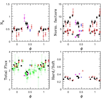
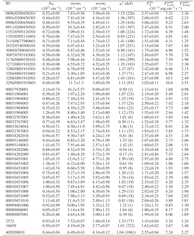
The results of these fits are provided in Table 2 and Fig. 3. The fitted fluxes (and the normalization factors) closely follow the count rates, as expected (see Fig. 2). The hardness ratios do not vary significantly, but the absorption clearly increases when the observed flux is low.
One XMM-Newton point is clearly an outlier, with a stronger flux (Table 2) and a harder spectrum (Table A.1) than other XMM-Newton data. This point corresponds to the exposure taken in Rev. 3097 (ObsID 0793183001). As mentioned in Section 2, Schulte 12 appears far off-axis in this observation and within stray light from Cyg X-3. Despite a careful selection of background, it therefore appears that the stray light contamina-tion cannot be totally eliminated. Therefore, we decided to dis-card these data from further consideration. We note that the spec-tra from the other off-axis observations (ObsID=0801910201– 601) appear less contaminated, with results usually within the errors (though they are far from perfect).
The Chandra and Swift data nicely agree with
XMM-Newton, despite some remaining cross-calibration uncertainties
(and a much larger noise for Swift), but the Suzaku results ap-pear discrepant, especially in flux and norm2 (the difference is
less significant for the other parameters and the hardness ratio also seems in agreement). That Suzaku dataset presented nei-ther an obvious stray light problem nor any reduction trouble. Furthermore, the closest XMM-Newton and Swift datasets, taken ∼200 d before and after the Suzaku dataset, respectively, agree well with the overall behaviour of Schulte 12; the origin of the
Suzakudiscrepancy therefore remains uncertain.
4. Optical results
4.1. Light-curve analysis
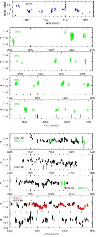
Gottlieb & Liller (1978) found Schulte 12 to be photometrically variable by up to 0.3 mag over decades while Laur et al. (2012)
0 0.5 1 0 0.5 1 1.5 0 0.5 1 0 5 10 15 0 0.5 1 0 0.2 0.4 0.6 0.8 1 0 0.5 1 0 1 2 3 4
Fig. 3.Results of the spectral fits: circumstellar absorption (top left), normalization factors (top right - the norm1 (resp. norm2)
values appear in the upper (resp. lower) part, with filled (resp. empty) circles for XMM-Newton data), observed flux (bottom left), and ratio of unabsorbed hard and soft fluxes (bottom right). The results for XMM-Newton data are shown as black circles except for the stray light-contaminated cases displayed as red triangles; magenta stars indicate Chandra data; blue crosses the
Suzakuobservation; and Swift data are shown as empty green
squares (shown for fluxes only). The phase folding is done as in Fig. 2.
and Salas et al. (2015) reported changes on shorter timescales. Laur et al. (2012) found no clear periodicity, only a typical vari-ation timescale of about 30 d. They also detected a potential trend in V − I colour, possibly linked to some spectral type varia-tions though systematic errors could not be excluded. In contrast, Salas et al. (2015) detected significant changes with an ampli-tude in the I filter of 0.18 mag and with a period of 54.0±0.1 d. This period is half the period found in X-rays, suggesting a com-mon origin with two photometric events per X-ray period.
The picture is however more complex when one looks at larger datasets. Our recent monitoring of the star was per-formed at the same time as the spectroscopic campaign (Fig. 4). It clearly confirms the brightness variations of Schulte 12, with minima occurring at HJD ∼ 2 458 315, 2 458 370, and 2 458 460.
Public photometric databases provide additional data. The noise affecting Hipparcos photometric measurements and Palomar Transient Finder (PTF) data renders them useless for detecting the small variations of Schulte 12, but significant vari-ations are found in the Northern Survey for Variable Stars (NSVS)6and in Integral-OMC7observations, though their time
coverage is scarce (Fig. 4).
ASAS-SN data8 (Shappee et al., 2014; Kochanek et al.,
2017) in the g and V filters taken on similar dates to our monitor-6 https://skydot.lanl.gov/nsvs/nsvs.php
7 http://sdc.cab.inta-csic.es/omc/ 8 https://asas-sn.osu.edu/
Table 2.Results of the spectral fits using models tbabs × phabs × P2apecwith temperatures fixed to kT1 =0.75 keV and kT2 =
1.9 keV.
ID NH norm1 norm2 χ2ν(dof) FobsX FunabsX,soft FX,hardunabs
(1022cm−2) (10−3cm−5) (10−3cm−5) (10−12erg cm−2s−1) 0896/0200450201 0.52±0.05 7.83±0.56 3.90±0.16 1.15 (226) 2.57±0.04 7.23 2.26 0901/0200450301 0.44±0.03 7.41±0.34 4.16±0.10 1.36 (397) 2.69±0.03 8.02 2.33 0906/0200450401 0.48±0.03 9.55±0.35 4.49±0.11 1.29 (416) 3.06±0.03 9.23 2.63 0911/0200450501 0.50±0.03 10.3±0.44 2.82±0.13 1.03 (307) 2.47±0.04 8.91 2.00 1353/0505110301 0.72±0.06 7.09±0.51 2.30±0.15 1.08 (224) 1.72±0.04 4.39 1.48 1355/0505110401 0.70±0.06 7.47±0.51 2.54±0.14 0.85 (221) 1.87±0.03 4.81 1.61 2114/0677980601 0.71±0.05 7.11±0.44 1.74±0.12 1.41 (108) 1.51±0.04 4.31 1.25 2625/0740300101 0.39±0.04 6.07±0.41 3.22±0.15 1.07 (251) 2.15±0.04 7.07 1.84 3089/0780040101 0.55±0.06 5.87±0.46 2.52±0.14 0.98 (181) 1.75±0.04 4.96 1.52 3097/0793183001 0.58±0.08 6.32±0.78 4.30±0.24 1.12 (107) 2.49±0.07 5.70 2.76 3176/0800150101 0.48±0.04 7.98±0.44 3.20±0.14 1.04 (299) 2.34±0.04 7.59 1.98 3273/0801910201 0.30±0.08 4.55±0.72 4.52±0.25 1.35 (103) 2.55±0.07 7.31 2.30 3280/0801910301 0.51±0.09 6.78±0.95 3.84±0.31 1.27 (87) 2.42±0.08 6.46 2.15 3284/0801910401 0.21±0.14 3.30±1.05 4.63±0.36 1.37 (71) 2.47±0.10 6.98 2.27 3288/0801910501 0.28±0.07 6.81±0.89 4.47±0.30 1.45 (101) 2.87±0.08 10.1 2.49 3294/0801910601 0.48±0.08 11.7±1.3 3.69±0.39 1.11 (83) 3.02±0.11 10.6 2.51 00037920001 2.14±0.74 16.2±5.57 0.00±0.93 0.50 (2) 1.12±0.41 1.68 0.98 00031904001 0.39±0.28 3.97±2.24 3.99±0.69 1.07 (23) 2.19±0.20 5.49 2.01 00031904002 0.80±0.32 7.10±2.91 2.41±0.74 1.25 (19) 1.72±0.16 3.91 1.52 00031904003 0.47±0.26 7.47±2.93 3.75±0.84 1.37 (25) 2.50±0.22 7.42 2.18 00031904004 0.35±0.32 4.10±2.25 3.46±0.64 0.61 (22) 2.01±0.17 5.73 1.80 00031904005 1.26±0.39 8.40±3.40 2.13±0.80 1.12 (15) 1.55±0.19 2.44 1.42 00032767001 0.36±0.64 1.40±4.24 3.62±1.45 1.01 (6) 1.69±0.43 3.03 1.64 00032767002 0.77±0.39 6.63±3.47 1.98±0.95 0.30 (11) 1.52±0.18 3.77 1.32 00033818044 0.50±0.71 8.50±11.9 3.99±3.75 1.86 (3) 2.71±0.72 8.01 2.36 00032767003 0.94±0.22 8.53±2.17 2.74±0.54 1.11 (37) 1.93±0.13 3.85 1.73 00034282018 0.94±0.57 9.30±7.65 4.24±2.19 0.81 (8) 2.57±0.49 4.51 2.38 00093146005 0.44±0.64 0.85±3.20 4.79±1.09 1.53 (8) 2.07±0.50 2.73 2.06 00093148003 1.41±0.73 7.91±6.44 2.57±1.63 1.42 (5) 1.60±0.33 2.06 1.51 00034282086 0.88±0.69 8.52±9.39 3.35±3.20 0.54 (4) 2.19±0.68 4.32 1.98 00034282089 0.01±0.87 1.40±8.29 5.72±2.39 0.17 (3) 2.81±0.84 7.53 2.64 00010451001 1.05±0.35 12.0±5.12 4.77±1.20 1.50 (18) 2.97±0.20 4.88 2.75 00010451002 1.38±0.71 6.22±6.00 3.26±1.33 0.61 (9) 1.69±0.24 1.86 1.66 00010451003 1.42±0.74 8.60±5.50 1.30±0.95 0.95 (8) 1.22±0.19 1.93 1.09 00010451004 0.75±0.42 5.27±3.19 2.86±0.79 1.28 (13) 1.71±0.20 3.48 1.57 00010451005 0.85±0.57 3.17±3.19 3.92±0.90 1.70 (14) 1.83±0.23 2.39 1.80 00010451006 1.00±0.32 9.67±3.89 4.13±0.98 1.02 (19) 2.53±0.23 4.28 2.35 00010451007 1.00±0.50 7.45±4.91 4.42±0.94 0.47 (18) 2.40±0.22 3.58 2.29 00010451008 0.16±0.54 1.08±2.80 4.30±0.76 1.29 (13) 2.02±0.25 4.24 1.94 00010451009 0.52±0.27 7.98±3.13 3.29±0.93 0.89 (18) 2.34±0.23 7.04 2.02 00010451010 1.11±0.45 11.4±5.33 2.49±1.13 0.81 (10) 2.04±0.26 3.89 1.81 00094061006 0.92±0.99 0.00±3.95 3.32±1.52 1.22 (1) 1.24±1.31 0.83 1.30 00088806001 0.05±0.67 3.14±4.91 2.90±1.33 1.64 (6) 1.80±0.35 8.17 1.55 00088807001 0.20±0.46 4.65±4.58 3.00±1.43 0.39 (6) 1.99±0.34 8.06 1.69 2572 0.93±0.14 7.52±0.87 1.68±0.14 1.33 (77) 1.43±0.04 3.24 1.24 16659 0.59±0.07 4.19±0.28 2.77±0.07 1.01 (722) 1.62±0.02 3.67 1.48 402030010 0.44±0.04 6.49±0.43 4.14±0.12 1.04 (1061) 2.55±0.04 7.24 2.27
Notes. Unabsorbed fluxes are corrected for the interstellar column (2.04 × 1022cm−2) only. Errors (found using the “error” command for the spectral parameters and the “flux err” command for the fluxes) correspond to 1σ; whenever errors were asymmetric, the largest value is provided here. Observed fluxes are expressed in the 0.5–10.0 keV band, while ISM-corrected fluxes are provided in the soft (0.5–2.0 keV) and hard (2.0– 10.0 keV) bands. For each dataset, all available data were fit simultaneously: EPIC-pn, MOS1, and MOS2 for XMM-Newton, zeroth and first orders for Chandra, XIS-0, 1, and 3 for Suzaku.
ing agree well with it (as well as with OMC data). The ASAS-SN data further reveal previous minima around HJD ∼ 2 458 240 and possibly 2 457 950 (Fig. 4). While the separation between the two minima in Summer 2018 is about 54 d, the previous min-ima occurred ∼75 d and 365 d earlier than HJD ∼ 2 458 315. In addition, the minimum of Fall 2018 occurred 145 d later than that date, so the interval between minima does not seem to be constant. Using the X-ray ephemeris, these five minima
corre-spond to phases of 0.86, 0.55, 0.24, 0.75, and 0.59 (considering the dates in chronological order). Only the third one (HJD ∼ 2 458 315) appears close to an X-ray minimum. Moreover, the photometric modulation seems to disappear at even earlier dates (HJD ∼ 2 457 000 − 800), with a long monotonic decrease de-tected between HJD ∼ 2 457 500 and HJD ∼ 2 457 800. No change in the ASAS-SN camera or observing strategy was per-formed however, meaning that this is not an instrumental effect.
1350 1400 1450 1500 9.1 9 8.9 NSVS HJD-245000 2600 2800 3000 3200 3400 11.8 11.6 11.4 OMC 3700 3800 3900 4000 11.8 11.6 11.4 OMC 4400 4600 4800 5000 11.8 11.6 11.4 OMC 5500 6000 6500 7000 11.8 11.6 11.4 OMC HJD-2450000 7000 7100 7200 7300 7400 11.8 11.7 ASAS-SN OMC+0.1 7400 7500 7600 7700 7800 11.8 11.7 ASAS-SN 7800 7900 8000 8100 8200 11.8 11.7 ASAS-SN OMC+0.1 11.8 11.7 ASAS-SN FC+0.1 8200 8300 8400 8500 13.5 13.4 13.3 HJD-2450000
Fig. 4.Photometry recorded by one of the present authors (F.C., red): ASAS-SN (black), OMC (green), and NSVS (blue). The times of the Hermes and Carmenes spectroscopic observations are indicated by solid blue and dashed cyan vertical tick sym-bols, respectively.
Salas et al. (2015) reported their detection of a periodic signal for observations taken in HJD ∼ 2 456 100 − 600. It therefore seems that the periodic signal may be transient.
Using the same methods as before, we performed a period search on the two largest datasets (ASAS-SN and OMC in V; see left panels of Fig. A.2). The periodogram based on
ASAS-SN data only shows a peak at very low frequencies, at a position close to a peak in the spectral window: no significant periodicity is therefore detected (as could be expected from the discussion above). On the other hand, the OMC periodogram possesses a clear peak at about 87 d, but the scarce time sampling does not fully cover a single 87 d period (i.e. there are no set of 5–10 points taken within 87 d): it is therefore difficult to fully con-firm it, and this signal could actually be related to the 54–108 d timescales. We also performed a period search on the most recent data only (last run of ASAS-SN data and our own photometric campaign; see right panels of Fig. A.2) since this is when the os-cillations are most apparent. While they cover similar time inter-vals (see Fig. 4), though with different sampling, the two datasets do not yield the exact same periodograms, with the highest peak at 73.6±2.2 d for ASAS-SN and at 48.4±1.1 d or 130±8 d for our own data. This confirms the probable absence of significant strict periodicity in the photometry, though significant variations on timescales of tens of days are clearly present.
4.2. Spectroscopic features
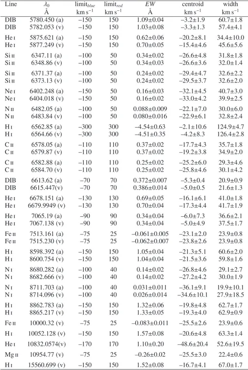
Apart from a large number of strong diffuse interstel-lar bands (DIBs, e.g. 5780, 5797, 6613 Å, Herbig, 1995), the optical and near-IR spectrum of Schulte 12 contains prominent hydrogen and He i lines, but also a few metal-lic lines (Fig. 5). In particular, Paschen and Brackett hy-drogen lines, He i λλ 5876, 6678, 7065Å, Si ii(+Mg ii) λ 6347Å, Si ii λ 6371Å, Ne i λ 6402 Å, N ii λ 6482 Å, C ii λλ 6578, 6583Å, O i λλ 7772, 7774, 8446Å, and N i λλ 8680–8718Å appear in ab-sorption, while He i λ 10830Å displays an incipient P-Cygni pro-file, Hα displays a strong emission, and Fe ii λ 7513, 9998Å and Mg ii λ 10952Å show weaker emissions.
Criteria for the spectral classification of OB supergiants based on red spectra in the region around Hα and in the I-band were discussed by Negueruela et al. (2010). In the spectrum of Schulte 12, the rather narrow Paschen lines as well as the rela-tive strength of the O i λ 8446 line compared to the neighbour-ing H i λ 8438 clearly indicate a mid-B supergiant star. On the other hand, the C ii lines are less constraining since they are strong for giants and especially so for supergiants of spectral types between B1 and B5 (Walborn, 1980; Negueruela et al., 2010). Although clearly present, the N ii λ 6482Å line is weak, suggesting a spectral type later than B2, which is confirmed by the presence of strong Si ii lines (Walborn, 1980). The presence of weak but definite N i lines in the region between 8680 and 8718 Å indicates a spectral type later than B3 but earlier than B6 (Negueruela et al., 2010). Comparing the equivalent widths (EWs) of Si ii λ 6347 and Ne i λ 6402 (EW = 0.34 ± 0.02 Å and 0.16 ± 0.02 Å, respectively - see Table 3) with the results of Lennon et al. (1993, Figs. 21 and 24) further yields a spec-tral type around B5 with an uncertainty or a range of varia-tion (see below) of about one subclass. The emission compo-nent of the He i λ 10830Å line is weaker than what is observed in very luminous (luminosity class Ia+) early B hypergiants
(Groh et al., 2007). The weak Fe ii λ 9998Å emission line was seen in the spectra of HD 183143 (B7 Ia) and µ Sgr (B8 Iap) pre-sented by Conti & Howarth (1999), but is absent in the spectrum of HD 225094 (B3 Ia) shown by the same authors. The above considerations suggest a spectral type B5 Ia for Schulte 12. This result is in reasonable agreement with the B3-4 Ia+
classifica-tion determined by Clark et al. (2012), except for the luminosity class. Whereas Clark et al. (2012) considered Schulte 12 to be a
Cyg OB2 12 on 2018 Aug 17 5800 5850 5900 0.6 0.8 1 1.2 6350 6400 0.8 1 6500 6550 6600 6650 0.5 1 1.5 7050 0.8 0.9 1 7500 1 1.05 7760 7780 0.8 1 8600 8700 8800 0.8 1 1.2 0.8 1 1.2 0.6 0.8 1 1.2
Wavelength (vac. calibrated) 0.8 1 -200 0 200 1 1.5 2 100626 131106 180502 180630 Velocity -200 -100 0 100 200 0.6 0.7 0.8 0.9 1 1.1 100626 131106 180502 180630 Velocity -200 -100 0 100 200 0.2 0.4 0.6 0.8 1 1.2 180502 180630 180825 Velocity -100 -50 0 50 0.95 1 1.05 1.1 1.15 180502 180630 180825 Velocity
Fig. 5. Left:Excerpts of the yellow-red and near-IR spectrum of Schulte 12, showing its main lines. Right: Examples of line profile variations.
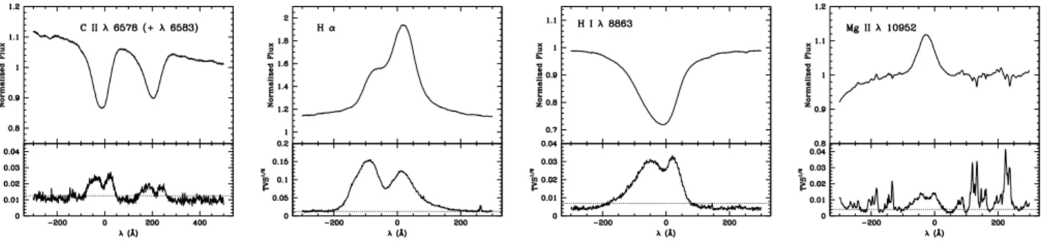
Fig. 6.Mean spectrum and temporal variance spectrum for various lines in the spectrum of Schulte 12. The dotted lines in the TVS1/2 panels correspond to the 1% significance level of variability evaluated accounting for the S/N of the data. On the sides of the Mg ii line, significant narrow variabilities are due to the imperfect correction of the telluric lines.
blue hypergiant, we favour a normal supergiant, which is also in line with the revised distance (see following section).
We compared the spectra taken close to minimum bright-ness (2018 May, July, and Sep) with those taken near maximum brightness (2018 June and mid-August). Several lines which are sensitive to spectral type (Lennon et al., 1993; Negueruela et al., 2010), and thus temperature, display changes of their strength that seem related to the brightness variations. For instance, the H i absorptions clearly appear stronger when the star is fainter and its V − I index is higher (Fig. A.3). A similar be-haviour, though of smaller amplitude, is seen in Ne i λ 6402Å, Si ii λλ 6347, 6371Å, and N i λ 8680Å. Correlated changes are less obvious for the C ii λλ 6578, 6583Å, and N ii λ 6482Å lines, but they are less sensitive to temperature effects. The observed variations suggest changes of the spectral type between about B4 and B6. Such variations of the temperature are consistent with the V − I colour variations of about 0.05 mag that we found to be correlated with the brightness variations of the star.
Our dataset is composed of 31 high-resolution spectra (of which 19 also cover the near-IR wavelengths) obtained between 2010 and 2018, with a denser monitoring over the last year (one spectrum every ∼10 d). Comparing these spectra, it is clear that line profiles change from one observation to the next (Fig. 5). At some point, most lines seem to skew and even become double, a telltale sign of binarity. However, in the process, the depths of these lines do not change significantly, contrary to what is seen in spectroscopic binaries. Furthermore, other lines observed simultaneously display no sign of splitting, such as the Mg ii and Fe ii emissions which simply seem to shift. Finally, Hα and He i λ 10830Å show a more complex behaviour. The Hα profile is mostly composed of a broad emission with one or two peaks. In the latter case, both the relative intensity of the two peaks and their separation may vary. In addition, a shallow blueshifted absorption is sometimes (but not always) present. These variations are much more extreme than those reported by Chentsov et al. (2013) and Klochkova & Chentsov (2004).
Finally, the He i λ 10830Å line profile is composed of three parts: a constant interstellar component (two deep and narrow absorp-tion lines at velocities ∼0 and –30km s−1), a broad emission
com-ponent on the red wing, and a complex absorption on both wings. When overplotting all data, the broad emission appears constant, whereas the absorption features vary in number, depth, width, and position.
To further characterise the variability, we computed the tem-poral variance spectrum (TVS, Fullerton et al., 1996) for the main lines mentioned above (see a few examples in Fig. 6). To this aim, we combined the Hermes and Carmenes spectral sets, which can be done in view of their similar resolving powers and of the fact that the line widths are largely dominated by the star, not the instrument. The TVS confirms the presence of signifi-cant variations over a large range of velocities, larger than the −vsin i to +v sin i range (v sin i = 38 km s−1, see Clark et al.,
2012). For all examined lines, the TVS displays a double-peaked structure. Such a profile is expected if the line centroid shifts back and forth in radial velocity. This can be the result of a gen-uine binary, pulsations, or co-rotating large-scale structures in the stellar wind. Another remarkable feature can be found when examining the symmetry of the TVS: the blue wing becomes progressively stronger when going from lines formed deep in the photosphere (such as the S ii or C ii lines which have roughly symmetric TVS profiles) to lines arising farther out (such as the hydrogen Paschen lines which have blue wings extending out to −150 km s−1). This probably reflects increasing contributions
from wind material to the absorption. The TVS of the Hα emis-sion line reveals the largest and broadest variability (up to 15% of the continuum, between –200 km s−1 and 150 km s−1), with
He i λ 10830Å being second (variations up to 9% in –150 km s−1
and 100 km s−1), but even the quieter Mg ii emission exhibits
changes by more than 1%.
To characterise the lines, fitting profiles of a given shape (e.g. Gaussian) is a usual method. However, because of the variabil-ity of the profiles, it is quite difficult to obtain a good fit over the full profile - only meaningful radial velocities can be de-rived by fitting the bottom (resp. top) of the absorption (resp. emission) lines. Therefore, we decided to focus on line mo-ments. Subtracting 1 from the normalized spectra, we calculated the zeroth-order moment M0 = P(Fi−1) which, multiplied
by the wavelength step, yields the EW, the first-order moment
M1 =P(Fi−1) × vi/P(Fi−1), which provides the centroid, and
the second-order moment M2=P(Fi−1)×(vi−M1)2/P(Fi−1),
whose square root gives the line width. Because of the noise, we avoided considering further orders. For each line, we limit the calculation to the wavelength interval where the line varies, us-ing most of the profile while avoidus-ing nearby lines. Table 3 dis-plays the averaged values of these moments (< X >= P Xi/N),
along with their dispersions (pP(Xi−<X >)2/(N − 1)). All
data were used in these averages, though a few noisy spectra (see Table 1) clearly add to the dispersion, especially for the bluer wavelengths. A very good agreement is found when comparing the two datasets, Carmenes and Hermes, demonstrating the re-liability of the reduction. The diffuse interstellar bands (DIBs) enable us to check the (small) “natural” noise around the mo-ment values, due to the number of collected photons and the quality of the reduction (wavelength calibration, normalization, etc.). This provides a threshold against which variability can be detected. Equivalent widths and widths generally are rather sta-ble except for the two lines strongly affected by wind, Hα and He i λ 10830Å. It is interesting to note that the dispersions in EW and width reach their smallest values not only for DIBs but also
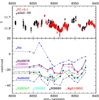
-40 -20 0 -40 -20 0 HeI7065 HeI5876 HeI10830 centroid(others) -40 -20 0 -40 -20 0 HI8598 HI8863 HI10052 HI15560 centroid(others) -40 -20 0 -40 -20 0 NeI6402 CII6578 NI8680 SiII6347 NII6482 centroid(others) -40 -20 0 -40 -20 0 MgII10952 FeII9998 FeII7513 DIB6613 centroid(others)
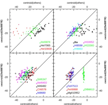
Fig. 7. Comparisons between the centroid of He i λ 6678Å and the centroids of other lines detected in the spectrum of Schulte 12 (He i lines on top left, H i lines on top right, and metallic absorp-tion and emission lines on bottom left and right, respectively). Filled symbols correspond to Hermes data, open symbols and crosses to Carmenes data; the diagonal yields the one-to-one cor-relation. For comparison, the case of a DIB is added to the last panel.
for Mg ii and Fe ii lines: this confirms that these stellar lines vary very little in shape. The centroids are however found to vary for all stellar lines, with the largest dispersions found for the wind lines and the smallest (again) for DIBs, and then for Mg ii and Fe ii emission lines.
To clarify the behaviour of the lines, we compared the individual centroids of different lines in Fig. 7. Except for the wind lines, strong correlations between centroids are found. But the devil lies in the details. Indeed, the amplitudes of variations fall into two groups: the centroids of He i λλ 5876, 6678, 7065Å, Si ii λλ 6347, 6371Å, C ii λλ 6578, 6583Å, and H i λλ 8598, 8863, 10052, 15560Å (all absorption lines) vary by about 25km s−1peak-to-peak, whereas
those of Fe ii λλ 7513, 9998Å, and Mg ii λ 10952Å emissions only change between –20 and –30km s−1. Indeed, a unity slope
can be used for all cases except when comparing centroids from the first group with those of the second (see bottom right panel of Fig. 7). However, it is also clear that even the variations of Fe ii and Mg ii are much larger than that observed for DIBs.
Rivinius et al. (1997) reported the results of an intense monitoring of three early-B hypergiants. All three stars dis-played significant velocity variations of their photospheric lines. For instance, in the case of ζ1Sco, Rivinius et al. (1997)
ob-served a pulsation-like pattern with a peak-to-peak amplitude of 20 km s−1on timescales near 10–15 d that gave way after some
time to a more random variation. Lines originating from outer layers of the photosphere were found to display a delayed varia-tion pattern compared to lines formed in deeper layers. In addi-tion, we may note that photometric variations with an amplitude near 0.1 mag were observed for ζ1Sco on the same timescales
Table 3.Average moments for different lines.
Line λ0 limitblue limitred EW centroid width
Å km s−1 km s−1 Å km s−1 km s−1 DIB 5780.450 (a) –150 150 1.09±0.04 –3.2±1.9 60.7±1.8 DIB 5782.053 (v) –150 150 1.03±0.08 –3.3±1.3 57.4±4.1 He i 5875.621 (a) –150 150 0.62±0.06 –20.2±8.1 34.4±10.0 He i 5877.249 (v) –150 150 0.70±0.05 –15.4±4.6 45.6±5.6 Si ii 6347.11 (a) –100 50 0.34±0.02 –26.6±4.8 31.8±1.8 Si ii 6348.86 (v) –100 50 0.34±0.03 –26.6±3.6 32.0±1.4 Si ii 6371.37 (a) –100 50 0.24±0.02 –29.4±4.7 32.6±2.2 Si ii 6373.13 (v) –100 50 0.24±0.02 –29.5±3.7 32.6±2.0 Ne i 6402.248 (a) –150 50 0.16±0.03 –32.1±4.5 40.7±3.0 Ne i 6404.018 (v) –150 50 0.16±0.02 –33.0±4.2 39.9±2.5 N ii 6482.05 (a) –100 50 0.088±0.009 –22.1±7.0 30.0±6.0 N ii 6483.84 (v) –100 50 0.080±0.016 –22.9±6.1 32.8±2.4 H i 6562.85 (a) –300 300 –4.54±0.63 –2.1±10.6 124.9±4.7 H i 6564.66 (v) –300 300 –4.51±0.35 –4.2±8.3 126.4±2.8 C ii 6578.05 (a) –110 110 0.37±0.02 –17.7±4.3 35.7±1.8 C ii 6579.87 (v) –110 110 0.37±0.02 –19.2±3.8 34.9±2.0 C ii 6582.88 (a) –110 110 0.25±0.02 –25.2±6.0 29.3±4.6 C ii 6584.70 (v) –110 110 0.25±0.02 –25.8±4.6 30.1±4.2 DIB 6613.62 (a) –70 70 0.372±0.007 –5.3±0.4 20.9±0.9 DIB 6615.447(v) –70 70 0.386±0.014 –5.0±0.5 21.6±1.3 He i 6678.151 (a) –130 130 0.69±0.05 –16.1±6.1 41.0±1.8 He i 6679.9949 (v) –130 130 0.70±0.04 –17.3±4.4 41.7±1.9 He i 7065.19 (a) –90 90 0.34±0.04 –6.0±7.3 36.6±2.1 He i 7067.138 (v) –90 90 0.34±0.04 –5.0±4.9 37.5±1.7 Fe ii 7513.161 (a) –75 25 –0.061±0.005 –23.1±2.0 23.9±0.8 Fe ii 7515.230 (v) –75 25 –0.062±0.007 –23.8±2.6 23.9±0.8 H i 8598.392 (a) –150 150 1.05±0.04 –21.3±5.1 60.6±2.0 H i 8600.754 (v) –150 150 1.04±0.04 –21.5±3.6 59.8±1.6 N i 8680.282 (a) –100 40 0.14±0.02 –26.8±4.6 29.1±2.7 N i 8682.666 (v) –100 40 0.14±0.02 –27.2±4.2 30.0±1.9 N i 8711.703 (a) –100 40 0.031±0.011 –36.1±9.1 19.9±10.1 N i 8714.096 (v) –100 40 0.026±0.014 –34.6±10.1 27.9±18.5 H i 8862.783 (a) –150 150 1.32±0.06 –19.8±4.8 62.7±1.7 H i 8865.217 (v) –150 150 1.33±0.05 –19.3±4.0 62.9±0.9 Fe ii 10000.32 (v) –75 25 –0.083±0.011 –25.5±2.6 23.9±0.6 H i 10052.128 (v) –150 150 1.57±0.08 –20.6±4.8 63.3±1.4 He i 10832.0574(v) –170 170 1.10±0.20 –48.6±20.4 52.6±19.5 Mg ii 10954.77 (v) –75 25 –0.26±0.02 –25.5±3.0 22.4±0.6 H i 15560.699 (v) –150 150 1.52±0.08 –16.7±4.1 67.0±1.7
Notes.Values are provided for the two sets of data separately, which is indicated in the rest wavelength column: Carmenes spectra were calibrated in vacuum (v) and Hermes data in the air (a) - usually wavelengths were taken from http://www.pa.uky.edu/∼peter/atomic/. EWs are negative for emission lines and positive for absorptions. As the C ii lines are in the red emission wing of Hα, moments were calculated considering a local continuum accounting for the emission wing.
Schulte 12 (though with a longer variation timescale, 50–100 d): the velocities of He i λ 6678Å and H i λ 8863Å lines display the same qualitative behaviour as those of C ii λλ 6578, 6583Å lines, but with a slight delay of the order of 3–5 d (see Fig. 8).
Finally, we performed period searches on the line profiles using the modified Fourier algorithm (Heck et al., 1985) and the same intervals as for the moment calculation. To this aim, we interpolated all profiles to a common velocity grid with steps of 0.2 km s−1, and then calculated periodograms at each velocity
considering the same velocity intervals as used for moment
cal-culations. These individual periodograms were then averaged to get a single periodogram per line (Fig. 9). While no frequency stands out, multiple peaks often appear near 0.015-0.025 d−1for
absorption lines, hinting at long-term variability on timescales of 40–65 days, that is, close to about half the X-ray period. Indeed, spectra taken only a few days apart (2017 May 24 and 29) show no significant difference while variations are detected on longer timescales, typically tens of days (see Figs. 4 and 8 - e.g. in the latter figure, the times of the two minimum velocities are sepa-rated by ∼50 d).
Fig. 8. Evolution of the photometry of Schulte 12 and of the centroids of some prominent lines in its spectrum during the Carmenes campaign in Summer 2018.
0 0.02 0.04 0.06 0.08 0.1 0.004 0.006 0.008 0.01 0.01 0.015 0.004 0.006 0.008 0.005 0.01 0.015 0.002 0.004 0.006 0.008 0 0.02 0.04 0.06 0.08 0.1 0.004 0.005 0.006 0.007
Fig. 9.Periodograms calculated on the line profiles (see text) for H i λλ 8598, 8663, 10052, 15560Å, He i λλ 5876, 6678, 7065Å, C ii λλ 6578, 6583Å, O i λλ 7772, 7774Å, Mg ii λ 10952Å, and the DIB at 6613Å for comparison. The vertical dotted line shows the frequency corresponding to the 108 d period.
5. Discussion
The previous sections led to several results. Firstly, at high ener-gies, the flux varies by a factor of about two and a period of 108 d is detected for these changes. The minimum flux corresponds to a time of lower intrinsic emission and increased absorption. Secondly, we confirmed the presence of photometric and spec-troscopic changes in the star, which we further constrained.
However, no regular clock seems present in the optical/near-IR domain, a simple timescale of 50–100 d being found. We now attempt to interpret these contrasting features.
5.1. The evolutionary status of Schulte 12
The second data release of GAIA (GAIA Collaboration, 2018) allowed for the first time a direct measurement of the par-allax of Schulte 12 to be made. This led to a surprising value of 1.18±0.13 mas. Indeed, this must be compared to the DR2 parallaxes of the other three main objects of the Cyg OB2 association, which are compatible with the usual distance used for Cyg OB2 (e.g. d ∼1.75 kpc in Clark et al., 2012): 0.64±0.06 mas for Cyg OB2 #5, 0.62±0.04 mas for Cyg OB2 #8A, and 0.60±0.03 mas for Cyg OB2 #9. Schulte 12 thus appears twice closer than the stars with which it is often as-sociated. Proper motions also appear quite different, with values of −1.9±0.2 mas in RA and −3.3±0.2 mas in DEC for Schulte 12 and values of minus 2.7–3.1 mas in RA and minus 4.1–4.7 mas in DEC for the others. This actually confirms early doubts on the membership of Schulte 12 to Cyg OB2 (Walborn, 1973).
One may however wonder whether or not the presence of vi-sual companions to Schulte 12 could impair the GAIA measure-ments. In this context, it is important to recall that all four X-ray bright massive stars of Cyg OB2 are actually multiple, with very diverse properties: Cyg OB2 #8A and 9 consist of spec-troscopic binaries with periods of 22 d and 2.4 yr, respectively, while Cyg OB2 #5 is thought to have four components with pe-riods ranging from 6.6 d to 9000 yrs. If companions were mod-ifying the parallax and proper motions of Schulte 12, it would be very surprising to find that the data of the other three sys-tems agree - but they do. Therefore the parallax difference of Schulte 12 is very probably real. In this context, one may also ar-gue that the angular diameter of Schulte 12 amounts to 1.31 mas, i.e. comparable to the parallax, as is the case of other blue super-giants (ζ1Sco, HD 190603, BP Cru, HD 80077, HD 168607, and
to a lesser extent P Cygni and HD 168625). Shifts in the pho-tocentre of the star (e.g. due to non-radial pulsations or spots on the stellar surface; see below) could thus affect the paral-lax. However, we note that the absence of a strong, strictly pe-riodic photometric modulation does not support this scenario. Furthermore, in view of the rather small relative error on the
GAIA-DR2 parallax, it would require an extraordinary
coinci-dence for the shifts of the photocentre to exactly mimic the ef-fect of an annual parallax in the GAIA data. We thus consider the revision of the distance as robust.
This new distance (840945
755pc in Bailer-Jones et al. 2018)
drastically changes the accepted physical properties of Schulte 12: scaling the values of Clark et al. (2012) yields a lu-minosity of log[LBOL/L⊙] = 5.64, a radius of 118 R⊙, and a
spectroscopic mass of 25 M⊙. The mass-loss rate proposed by
Clark et al. (2012) or Morford et al. (2016) would also be re-duced by about a factor of four. Schulte 12 now appears as a normal supergiant, without any luminosity problem (a difficulty noted by Clark et al., 2012).
It is interesting to compare Schulte 12 with the LBV R 71 in the Large Magellanic Cloud which is at the lower luminosity end of the classical LBV strip (Mehner et al., 2017). Both stars share similar properties (Mehner et al., 2017; Clark et al., 2012, and this work): they have similar spectroscopic masses (27 M⊙
for R 71 and 26 M⊙for Schulte 12), temperatures (15 500±500 K
for R 71 in quiescence and 13 700+800
−500K for Schulte 12), radii
(107 R⊙for R 71 in quiescence and 118 R⊙for Schulte 12), and
luminosities (6.0 105L
Fig. 10.Tentative orbital solution of Schulte 12 for a fixed orbital period of 108 d (middle column of Table 4). The average veloc-ities of Mg ii and Fe ii emissions in the Carmenes dataset are shown by black dots and the Hermes velocities of Fe ii λ 7513Å (not used to obtain the orbital solution) by open red squares. We note that the phase used here corresponds to the binary ephemeris (Table 4), not to the X-ray ephemeris used for Figs. 2 and 3.
for Schulte 12). The slight luminosity difference is sufficient to keep Schulte 12 outside of the LBV strip, but actually close to it, while R 71 lies inside of it. Evidence that Schulte 12 is less evolved than R 71 comes from the chemical composition of its atmosphere. Mehner et al. (2017) reported a strong enrichment of the atmosphere of R 71 with CNO processed material (with number ratios of He/H = 0.20, O/N = 0.08 and C/N = 0.05). For Schulte 12, Clark et al. (2012) derived a significantly weaker enrichment (He/H = 0.1, O/N = 1.48, C/N = 0.31).
5.2. Binarity
As already mentioned in Section 4.2, the changing profile of the absorption lines cannot be due to line blending as the profile broadens, skews, or becomes narrower without much changes in line depth (Fig. 5). However, the Mg ii and Fe ii emissions un-dergo simple velocity shifts, which could be interpreted in this framework. Combining the centroid velocities of the Mg ii and Fe ii emission lines, we computed using LOSP9 a highly
pre-liminary orbital solution. In this calculation, we assume that the 108 d X-ray period is linked to orbital motion. Freeing the pe-riod does not significantly change the quality of the fit or the values of the orbital parameters. The results are given in Table 4 and illustrated in Fig. 10. The periastron passage of this tentative orbit occurs ∼10 d (or ∆(φ) =0.1) after the X-ray maximum and ∆(φ) =0.25 before the X-ray minimum - in colliding-wind bina-ries however the periastron usually corresponds quite closely to an X-ray extremum.
9 LOSP (Sana et al., 2006) is an improved version of the code
origi-nally proposed by Wolfe et al. (1967).
Table 4. Tentative orbital solution built from the mean RVs of the Mg ii λ 10952Å and Fe ii λλ 7513, 9998Å emission lines (Carmenes data only).
Porb(days) 108.0 (fixed) 104.1 ± 5.7
γ(km s−1) −25.2 ± 0.5 −25.2 ± 0.5 K(km s−1) 3.3 ± 0.8 3.3 ± 0.8 e 0.55 ± 0.20 0.53 ± 0.20 ω(◦) 193 ± 23 197 ± 25 T0(HJD−2 450 000) 8299.8 ± 5.4 8300.4 ± 5.9 asin i (R⊙) 5.9 ± 1.7 5.8 ± 1.6 f(m) (M⊙) 0.00024 ± 0.00020 0.00024 ± 0.00046 rms (km s−1) 1.7 1.7
If we assume Schulte 12 to be a binary system, we need to ask ourselves whether or not the spectroscopic radius of the B supergiant is consistent with the radius of its Roche lobe. For this purpose, we use the formula of Eggleton (1983) to express the dependence of the Roche lobe radius on the mass-ratio q = m1 m2 as follows: RRL R⊙ = 2.06 q 2/3 0.6 q2/3+ln (1 + q1/3) 1 + q q !1/3 m 1 M⊙ !1/3 P day !2/3 .(1) If we adopt a period of 108 d and a spectroscopic mass of
m1 = 25 M⊙ for the B supergiant, we find that the radius of
the Roche lobe of the B supergiant exceeds 127 R⊙whatever the
value of q. Therefore, if the orbit were circular, the spectroscopic radius of 118 R⊙would fit entirely into the Roche lobe. The B
supergiant would fill less than 80% of the volume of its Roche lobe, regardless of the mass of its companion. However, this is valid for a circular orbit, not in the presence of a significant or-bital eccentricity as found here. Assuming that in a long-period eccentric binary the size of the Roche lobe varies in proportion to the instantaneous orbital separation, we find that for an eccen-tricity of about 0.5 (Table 4) the B supergiant would significantly overflow its Roche lobe at phases near periastron, regardless of the value of the mass of the companion.
Nevertheless, there is a significant dispersion of the data points around the best-fit curve, and moreover, plotting the addi-tional Fe ii λ 7513Å velocities measured on Hermes spectra does not reveal a coherent behaviour (Fig. 10). It must be underlined here once again that Hermes and Carmenes spectra agree well: the spectra taken in May 2017 with both instruments at only a 5 d time difference appear very similar while the DIB centroids coincide within errors (see Table 3). Therefore, no problem in the instrument or during the analysis can be blamed for the dif-ference observed in Fig. 10. In fact, no orbital solution using the full Fe ii λ 7513Å velocity dataset can be derived as these data simply cannot be reconciled with a 108 d period. Combined to the partial correlation of the emission line velocities with those of absorptions (Figs. 7 and 8), this suggests that we are not wit-nessing pure orbital motion. If Schulte 12 is a binary, we have not yet found evidence for it in the RVs.
Finally, we examined the spectrum of Schulte 12 in search of lines moving in the opposite direction compared to Mg ii or of lines with a different ionization (e.g. He ii), as they could then be attributed to a companion. None were found however. With the revised distance of Schulte 12, its absolute V-band magni-tude amounts to −8.26. We estimate that our spectroscopic data should enable us to detect the spectroscopic signature of an O-type companion down to 2.5 magnitudes fainter than the B super-giant. Considering the typical parameters of O-type stars from the calibration of Martins et al. (2005), we conclude that a
main-Fig. 11. Revised position of Schulte 12 in the Hertzsprung-Russell diagram adopting the distance corresponding to the
GAIA-DR2 parallax. The evolutionary tracks are taken from
Ekstr¨om et al. (2012) for solar metallicity and no rotation. The continuous red line corresponds to the empirical Humphreys-Davidson limit (Humphreys & Humphreys-Davidson, 1994). Various insta-bility boundaries are shown according to Saio (2011). The dot-ted red curve indicates the instability boundary of low-order ra-dial and non-rara-dial p-mode oscillations. The short-dashed ma-genta contour indicates the region where non-radial g-modes with ℓ ≤ 2 are excited by the iron opacity bump. Finally, the cyan long-dashed contour indicates the region where oscillatory convection modes with ℓ ≤ 2 are excited (Saio, 2011).
sequence O-type star would remain entirely hidden, regardless of its spectral type. For O-type giants, only objects with a spectral type earlier than O5 would show up in the combined spectrum. Finally, O supergiants should be detectable in a combined spec-trum regardless of the spectral types. The non-detection of even a massive companion would therefore not be entirely surprising. 5.3. Pulsational activity
The erratic variations of the centroids and profiles of the absorp-tion lines suggest that the velocities of these lines are dominated by effects other than genuine orbital motion. One explanation for these variations could be non-radial pulsations of the B su-pergiant; but is Schulte 12 expected to be pulsationally unstable? With the revised physical properties, the position of Schulte 12 in the Hertzsprung-Russell diagram (Fig. 11) drasti-cally changes. The star now appears relatively far away from the empirical Humphreys-Davidson limit (Humphreys & Davidson, 1994) and thus from the region where strange-mode oscillations are expected (Kiriakidis et al., 1993). Maeder (1980) suggested that intermediate term variability of B – G supergiants could stem from non-radial gravity-mode pulsations connected to a large outer convection zone. Indeed, Schulte 12 is located within the part of the Hertzsprung-Russell diagram where oscillatory convection modes with ℓ ≤ 2 are expected (Saio, 2011). If we attribute the photometric variability of Schulte 12 to non-radial
pulsations, they must indeed be of low ℓ to explain the relatively large observed amplitude of the variations. For a 30 M⊙star, Saio
(2011) predicts periods of excited ℓ = 1 and ℓ = 2 modes of about 70 and 60 days, respectively. These values are reasonably close to the timescale of the variations of the absorption lines and the photometry of Schulte 12. Furthermore, the pulsation modes are associated to subphotospheric convection which is known to be unstable, hence the pulsational activity could be intermittent, and they have growth timescales comparable to their period, sug-gesting that such (dis)appearance could occur quite quickly, in line with our observations of Schulte 12.
The line profile variability (LPV) of absorption lines due to non-radial pulsations depends on the ratio k between the az-imuthal and radial pulsation velocities (Kambe & Osaki, 1988). The fact that the strongest LPV signatures are observed in the cores of the lines (see Fig. 6), suggests that k << 1. Schulte 12 lies also at the edge of the zone where low-order (n = 0 or n = 1) radial pressure modes are expected to be excited according to Jeffery & Saio (2016). However, the corresponding fundamental (n = 0) radial modes should have periods of order 106s, that
is about 12 days, which is much shorter than the observed peri-ods. It seems therefore unlikely that the observed variability of Schulte 12 could arise from such radial modes.
At this stage, it is once more interesting to compare Schulte 12 with the LBV R 71. During quiescence, R 71 dis-plays microvariations of 0.1 mag amplitude on timescales of 14 – 100 days (Mehner et al., 2017, and references therein). This is qualitatively similar to what we observe in Schulte 12, prob-ably indicating that both stars are subject to similar pulsation mechanisms. During the currently ongoing outburst of R 71, a new kind of nearly periodic photometric variation appeared, consisting of oscillations of 0.2 mag amplitude on a timescale of about 445 days (Walborn et al., 2017; Mehner et al., 2017). The star R 71 currently displays a late F supergiant spectrum (Walborn et al., 2017; Mehner et al., 2017), very different from that of Schulte 12. However, an interesting point concerns the spectroscopic variability that occurs on a timescale twice that of the above-mentioned 445-day photometric cycle. Indeed, the absorption lines vary between single and double morphologies (Mehner et al., 2017; Walborn et al., 2017), in a way similar to what we observe for Schulte 12. By analogy with RV Tau vari-ables, Mehner et al. (2017) attribute the line doubling to shock waves triggered by the pulsations and propagating through the atmosphere of R 71. Whether a similar explanation holds in our case is unclear, as the atmospheric structure of the B5 Ia giant Schulte 12 is rather different from that of a late-F super-giant.
5.4. The X-ray clock
The X-ray data for Schulte 12 display a clear periodicity of 108 d. This is incompatible with the putative periods of the visual companions (see Introduction), and therefore they do not play a role in this phenomenon. The question then arises regarding the origin of the high-energy emission.
The folded X-ray light curve of Schulte 12 is strongly rem-iniscent of that of the massive binary WR 21a, where X-rays arise in the collision between the stellar winds of the two stars (Gosset & Naz´e, 2016). As in Schulte 12, the count rate remains relatively constant most of the time (or slightly increases), then a stronger increase occurs, followed by a sharp drop and a longer recovery. In WR 21a, the increase was associated to the typi-cal 1/D increase in flux found in adiabatic wind–wind collisions as stars approach periastron (Stevens et al., 1992). The