Using Partial Orders for the Efficient Verification of
Deadlock Freedom and Safety Properties
Patrice Godefroid Pierre Wolper Universit´e de Li`ege
Institut Montefiore, B28 4000 Li`ege Sart-Tilman, Belgium Email: {god,pw}@montefiore.ulg.ac.be Formal Methods in System Design, Kluwer Academic Publishers, 2(2):149--164, April 1993.
Abstract
This paper presents an algorithm for detecting deadlocks in concurrent finite-state sys-tems without incurring most of the state explosion due to the modeling of concurrency by interleaving. For systems that have a high level of concurrency our algorithm can be much more efficient than the classical exploration of the whole state space. Finally, we show that our algorithm can also be used for verifying arbitrary safety properties.
1
Introduction
When reasoning assertionally about concurrent programs, separating safety and liveness prop-erties is a well established paradigm [1, 2]. Indeed, the proof techniques used for these two types of properties are quite different: safety properties are mostly established with invariance arguments whereas liveness properties require the use of well-founded orders.
Surprisingly, this distinction can often be ignored in model-checking [3, 4, 5, 6]. Indeed, model checking can handle arbitrary temporal formulas which can represent both safety and liveness properties. Nevertheless, it has been noticed that restricting model-checking like techniques to safety properties can lead to better verification algorithms [7, 8, 9]. Intuitively, this can be understood by the fact that safety properties can be checked by only considering the finite behaviors of a system whereas liveness properties are only meaningful for infinite behaviors. Representing infinite behaviors requires the use of concepts such as automata on infinite words or trees [10, 11] which are significantly harder to manipulate than their finite word or tree counterparts [12, 13].
In this paper, we explore whether partial-order model-checking techniques such as those of [14, 15] also benefit from being restricted to safety properties. The motivation for partial-order verification methods is that representing concurrency by interleaving is usually semantically adequate but quite often extremely wasteful. This wastefulness plagues model checking as well as other finite-state verification techniques since it creeps in when constructing the global state graph corresponding to a concurrent program. In [16, 17, 18] among others, it is shown that most of the state explosion due to the modeling of concurrency by interleaving can be avoided. For instance, the method used in [16] is to build a state-graph where usually only one (rather
than all) interleaving of the execution of concurrent events is represented. This reduced state-graph can then still be viewed as correctly representing the concurrent program by giving it an interpretation based on Mazurkiewicz’s trace theory [19].
We first turn to the grand-father of finite-state verification problems: deadlock detection. We show that for this problem, the algorithm of [16] can be strongly simplified and improved. The main idea of the simplification (which is also found in [20]) is that since we are seeking deadlocks, one can generate a global representation of the program that chooses amongst independent events in a completely arbitrary way. The choices can even be completely “unfair” since, if there is a deadlock, favored processes will anyway eventually be blocked and the deadlock will be detected. This simplification leads to an algorithm that can be more easily and efficiently implemented than the one of [16] and that often generates substantially fewer states.
Our next step is to turn to the verification of general safety properties. The approach we use here is that of “on the fly verification” [6, 21, 9, 22, 23, 24]. Namely, we represent the safety property (or rather its complement) by an automaton on finite words and we check that the accepting states of this automaton are not accessible in its product with the automata representing the program. We thus reduce the problem of verifying safety properties to a state accessibility problem. This problem is in turn reduced by a simple transformation of the program and of the specification to a deadlock detection problem to which we apply our new algorithm.
The paper ends with a comparison between our contributions and related work.
2
A Representation of Concurrent Systems
We consider a concurrent program P composed of n concurrent processes Pi. Each process is
described by a finite automaton Ai on finite words over an alphabet Σi. Formally, an automaton
is a tuple A = (Σ, S, ∆, s0), where Σ is an alphabet, S is a finite set of states, ∆ ⊆ S × Σ × S is
a transition relation, and s0∈ S is the starting state.
We consider automata without acceptance conditions. Thus a word w = a0a1. . . an−1 is
accepted by an automaton A if there is a sequence of states σ = s0. . . sn such that s0 is the
starting state of A and, for all 0 ≤ i ≤ n − 1, (si, ai, si+1) ∈ ∆. We call such a sequence σ an
execution of A on w. A state s is reachable from s0 if there is some word w = a0a1. . . an−1 and
some execution σ = s0. . . sn of A on w such that s = sn.
An automaton AG representing the joint global behavior of the processes Pi can be
com-puted by taking the product of the automata describing each process. Actions that appear in several processes are synchronized, others are interleaved. Formally, the product (×) of two (generalization to the product of n automata is immediate) automata A1 = (Σ1, S1, ∆1, s01) and
A2= (Σ2, S2, ∆2, s02) is the automaton A = (Σ, S, ∆, s0) defined by
• Σ = Σ1∪ Σ2, • S = S1× S2, s0 = (s01, s02), • ((s, t), a, (u, v)) ∈ ∆ when – a ∈ Σ1∩ Σ2 and (s, a, u) ∈ ∆1 and (t, a, v) ∈ ∆2, – a ∈ Σ1\ Σ2 and (s, a, u) ∈ ∆1 and v = t, – a ∈ Σ2\ Σ1 and u = s and (t, a, v) ∈ ∆2.
Let S = S1 × · · · × Sn and ∆ ⊆ S × Σ × S denote respectively the set of states and the
transition relation of the product AG of the n automata Ai. In what follows, we assume that
the sets of states Si of the automata Ai are pairwise disjoint and, for a state s = (s1, s2, . . . , sn)
of AG, we write s ∈ s to mean ∃i, 1 ≤ i ≤ n such that s = si, i.e. we allow ourselves to view
the state s as a set rather than as a vector. Then, for each transition t = (s, a, s0) ∈ ∆ with s = (s1, s2, . . . , sn) and s0 = (s01, s02, . . . , s0n), the sets
- •t = {si∈ s : (si, a, s0i) ∈ ∆i},
- t•= {s0i∈ s0 : (si, a, s0i) ∈ ∆i} and
- •t•= •t ∪ t•
are called respectively the preset , the postset and the proximity of the transition t. Intuitively, the preset , resp. the postset , of a transition t = (s, a, s0) of AG represents the states of the Ai’s
that synchronize together on a, respectively before and after this transition. We say that the Ai’s with a nonempty preset and postset for a transition t are active for this transition. The
state s0 reached after the execution of a transition t from a state s is s0= (s \•t) ∪ t•.
Two transitions t1= (s1, a1, s01), t2 = (s2, a2, s02) ∈ ∆ are said to be equivalent (notation ≡)
iff
•t
1=•t2∧ t•1= t•2∧ a1 = a2.
Intuitively, two equivalent transitions represent the same transition but correspond to distinct occurrences of this transition. These occurrences can only differ by the states of the Ai’s that
are not active for the transition. We denote by T the set of equivalence classes defined over ∆ by ≡. In the sequel, “transitions” will denote elements of T .
3
Efficiently Detecting Deadlocks
A deadlock in a system composed of n concurrent processes Pi is defined as a reachable state
of the system in which all processes Pi are blocked, i.e. where no transition is executable.
Detecting deadlocks is usually performed by an exhaustive enumeration of all reachable states of the automaton AG corresponding to the product of the n automata Ai. This enumeration
amounts to exploring all possible transition sequences the system is able to perform and storing all intermediate states reached during this exploration. In concurrent systems, the number of reachable states can be very large: this is the well-known “state explosion” phenomenon. This combinatorial explosion limits both the applicability and the efficiency of the classical method. In this section, we present a new simple method for detecting deadlocks without computing and storing all reachable states of the concurrent system. The basic idea is to describe the behavior of the system by means of partial orders rather than by sequences. More precisely, we use Mazurkiewicz’s traces [19] as a semantic model.
Traces are defined as equivalence classes of sequences. Given an alphabet Σ and a dependency relation D ⊆ Σ × Σ, two sequences over Σ belong to the same trace with respect to D (are in the same equivalence class) if they can be obtained from each other by successively exchanging adjacent symbols which are independent according to D. For instance, if a and b are two symbols of Σ which are independent according to D, the sequences ab and ba belong to the same trace. A trace is usually represented by one of its elements enclosed within brackets and, when necessary,
subscripted by the alphabet and the dependency relation. Thus the trace containing both ab and ba could be represented by [ab](Σ,D). A trace corresponds to a partial ordering of symbol
occurrences and represents all linearizations of this partial order. If two independent symbols occur next to each other in a sequence of a trace, the order of their occurrence is irrelevant since they occur concurrently in the partial order corresponding to that trace.
To describe the behavior of the concurrent system represented by AG in terms of traces, we
define the dependency in AG as the relation DAG ⊆ T × T such that
(t1, t2) ∈ DAG iff
•
t•1∩•t•2 6= ∅.
The complement of DAGis called the independency in AG. Given an alphabet and a dependency
relation, a trace is fully characterized by only one of its linearizations (sequences). Thus, given the set of transitions T and the dependency relation DAG defined above, the linear behaviors of
AG can be fully investigated by exploring only one sequence (interleaving) for each possible trace
(partial ordering of transitions) the system is able to perform.
Note that all deadlocks of AG will be detected during this exploration. Indeed, for each
deadlock, there exists at least one transition sequence w leading to this deadlock from the starting state. Moreover, all other sequences belonging to the same equivalence class [w](T ,DAG)
also lead to the same deadlock. Thus, for detecting this deadlock, it is sufficient to explore only one of these sequences which can be chosen arbitrarily. This deadlock-preserving property of partial-order semantics was already pointed out in [25, 20] among others.
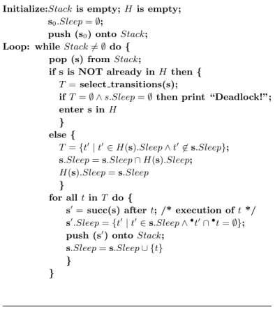
Figure 1 presents an algorithm for performing this exploration. The main data structures used are a Stack to hold the states from which the behavior of the system remains to be investigated, and a hash table H to store the states that have already been visited. This algorithm looks like a classical exploration of all possible transition sequences, except for two differences. The first difference is that, instead of executing systematically all transitions enabled in a state, we choose only some of these transitions to be executed. The second difference is that a sleep set is attached to every state in order to further limit the search. Let us first examine the selection of transitions.
The basic idea for selecting amongst the enabled transitions those that have to be executed is the following. Whenever several independent transitions are enabled at a given state, we execute only one of these transitions. This will ensure that we generate only one interleaving of these independent transitions. When enabled transitions are dependent, their executions lead to different traces corresponding to different nondeterministic choices which can be made by the system. We then have to execute all these transitions in order to consider all possible traces the system is able to perform.
We now give more details. In what follows, two transitions t1, t2 are referred to as being
in conflict iff (•t1 ∩•t2) 6= ∅. Checking if two enabled transitions are dependent can be done
by checking if they are in conflict. Indeed, if two enabled transitions are in conflict, they are trivially dependent. Conversely, two dependent transitions have at least one active process in common and, if they are simultaneously enabled, this implies that they are in conflict. Two transitions t, t0 are in indirect conflict iff ∃t1, . . . , tn, n ≥ 1 : (•t ∩•t1) 6= ∅ ∧ (•t1 ∩•t2) 6=
∅ ∧ . . . ∧ (•tn−1∩•tn) 6= ∅ ∧ (•tn∩•t0) 6= ∅.
Two cases can occur in the selection of transitions.
1. There is a transition that is only in conflict or indirect conflict with enabled transitions. Then, this transition and all the transitions that are in conflict or indirect conflict with
Initialize:Stack is empty; H is empty; s0.Sleep = ∅;
push (s0) onto Stack;
Loop: while Stack 6= ∅ do { pop (s) from Stack;
if s is NOT already in H then { T = select transitions(s);
if T = ∅ ∧ s.Sleep = ∅ then print “Deadlock!”; enter s in H
} else {
T = {t0| t0∈ H(s).Sleep ∧ t06∈ s.Sleep};
s.Sleep = s.Sleep ∩ H(s).Sleep; H(s).Sleep = s.Sleep
}
for all t in T do {
s0= succ(s) after t; /* execution of t */ s0.Sleep = {t0| t0∈ s.Sleep ∧•t0∩•t = ∅}; push (s0) onto Stack;
s.Sleep = s.Sleep ∪ {t} }
}
Figure 1: Deadlock Detection Algorithm
it are selected. Indeed, these transitions are independent with respect to the rest of the system and their occurrence can not be influenced by it. An interesting special case is that of an enabled transition that is not in conflict with any other transition. In this situation, this transition alone is selected.
2. There is no transition that is only in conflict or indirect conflict with enabled transitions, i.e. each transition is in conflict or indirect conflict with at least one disabled transition. In this case all enabled transitions are explored. Indeed, let t be an enabled transition that is in conflict with a transition x that is not enabled in the current state (this is a situation of confusion [26]). It is possible that x will become enabled later because of the execution of some other transitions independent with t. At that time, the execution of t could be replaced by the execution of x. Thus when we select t, we also have to check if the execution of t could be replaced by the execution of x after the execution of some other enabled transitions independent with t (i.e. to check if the confusion actually leads to a conflict): we thus have to select all enabled transitions that are dependent (as usual) and independent with t, i.e. all enabled transitions.
The selection procedure we have given can lead to independent transitions simultaneously being selected. This can cause the wasteful exploration of several interleavings of these transi-tions, for instance when a case of confusion does not lead to a conflict. Sleep sets are introduced to control this wastefulness. Imagine, for instance, that we have a situation of confusion with
select transitions(s) { T = enabled(s)\s.Sleep;
if ∃t ∈ T :conflict(t)⊆ enabled(s) then selection= {t} ∪ (conflict(t)∩T ); else selection= T ;
return(T ) }
Figure 2: Selection Amongst Enabled Transitions
two enabled independent transitions a and b, and that a is in conflict with only one disabled transition c. We have to explore both the result of transition a and of transition b. Choosing transition a amounts to choosing one interleaving of a and b to be explored. The purpose of exploring the result of transition b is to check if it will eventually enable the transition c with which a is in conflict. So, when doing this, there is no point in exploring the result of transi-tion a. Thus, sleep sets are used to prevent the executransi-tion of a in the states reached after the execution of transition b.
More precisely, a sleep set is a set of transitions. One sleep set is computed for each state s reached during the search. The sleep set computed for a state s is a set of transitions that are enabled in s but will not be executed from s. The sleep set associated with the initial state s0 is the empty set. The sleep sets of the successors of a state s are then computed as follows.
Let us call t1 the first transition that is explored from s. The sleep set associated with the state
reached by t1 is the sleep set of s unmodified except for the elimination of transitions that are
dependent with t1. When the exploration of t1 is finished, it is added to the sleep set of s. Thus,
the transition t1 will also be added to the sleep set of the state reached by the next transition
(say t2) as long as it is not dependent with it. One then proceeds in a similar way with the
remaining transitions. The general rule is thus that the sleep set of a state s0 reached by a transition t from a state s is the sleep set that was obtained when reaching s augmented with all transitions already explored from s and purged of all transitions that are dependent with t. Let us now see how the selection procedure we have described is implemented in the algorithm of Figure 2. The function conflict(t) returns the transitions that are in conflict and indirect conflict with t. The function enabled(s) returns all enabled transitions in state s. The first step is to ignore the transitions that are in the sleep set s.Sleep associated with the current state s. If there is a transition t among the remaining enabled transitions such that all transitions in conflict(t) are enabled, then t and the transitions of conflict(t) that are not in the current sleep set are selected (in practice, if there are several such enabled transitions, one chooses one that minimizes the number of transitions in the selection set). The other remaining possibility is that of a case of confusion in which all enabled transitions that are not in the sleep set are selected.
The algorithm of Figure 1 includes all operations required to manipulate sleep sets. This al-gorithm performs a call to the function select transitions each time a new state is encountered during the search. If a state has already been visited with a sleep set H(s).Sleep containing transitions that are not in the current sleep set s.Sleep, these transitions are explored (see
Classical Algorithm New Algorithm
States Trans. States Trans.
rr4 144 368 20 24
rr5 360 1100 25 30
rr6 864 3072 30 36
rr7 2016 8176 35 42
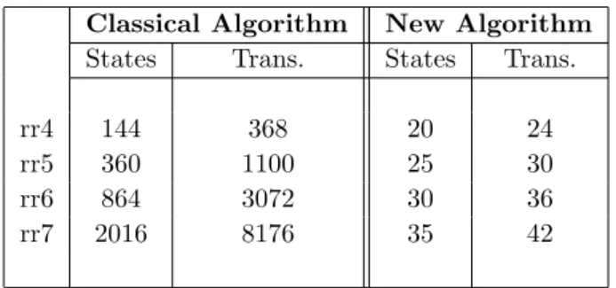
Table 1: Analysis of the Round Robin Access Protocol
Appendix for details).
All this ensures that sufficient interleavings of the traces the system can perform are explored, while still avoiding the construction of all possible interleavings of enabled independent transi-tions. Proofs of the correctness of the algorithm can be found in Appendix A. The practical advantage of the algorithm presented here is that, by construction, the state-graph G0 explored by this algorithm is a “sub-graph” of the usual state-graph G representing all possible transition sequences of the system. (By sub-graph, we mean that the states of G0 are states of G and the transitions of G0 are transitions of G.) Moreover, the function select transitions required for constructing G0 can be implemented in such a way that the order of its time complexity is the same as the one of the function enabled that is used to construct G. Thus our algorithm never uses more resources than (i.e. has the same worst-case asymptotic complexity as) the classical state space exploration algorithm and is often much more efficient in practice. Of course, if no simultaneous enabled independent transitions are encountered during the search, our method becomes equivalent to the classical one.
Table 1 compares the performance of a classical depth-first search algorithm against the deadlock detection algorithm presented in this section for analyzing the Round Robin Access Protocol described in [27] for a ring of 4 (rr4) to 7 (rr7) participants. One clearly sees that our method explores a much smaller number of states and transitions than the classical one. With our method, the number of states and transitions that need to be explored to conclude that the protocol is deadlock-free grows in a linear way with the number of participants in the protocol. The algorithm presented in this paper is a simplified and improved version of the one pre-sented in [16] that was designed to generate at least one interleaving for each possible trace of a concurrent program. The simplification comes essentially from the fact that, when looking for deadlocks, if the algorithm detects that one of the concurrent processes can loop in the current trace being explored, the exploration of this trace can stop without generating the remainder of this trace as it had to be done in [16]. Hence, the number of explored states and transitions with the new algorithm presented here is always less than or equal to the number explored with the algorithm described in [16].
4
Verifying Safety Properties
In this section, we show how the reachability of a global state, the reachability of a local state, and finally the verification of a safety property can be reduced to deadlock detection. Note that
we cannot directly use the algorithm of Section 3 to determine reachability since it usually does not generate all reachable states.
The algorithm presented in the previous section can easily be used to check if a given global state s = (s1, s2, . . . , sn) of a concurrent program P is reachable. This is done by adding
to all Ai’s a transition (si, δ, stopi) for si ∈ s. We call the modified system PM. Then, the
state s0 = (stop1, stop2, . . . , stopn) is a deadlock of PM iff the state s is reachable. Indeed, the
synchronization of all processes on the transition δ leading to s0 in PM is possible only if the
global state s is reachable. Hence checking the reachability of s amounts to checking if s0 is a deadlock of the modified system PM.
Let us now turn to the problem of checking the reachability of a given local state `. A local state is defined as an incompletely specified global state. In other words, it is a tuple of states of some (but not all) processes. For convenience, we define a local state ` as a subset of S
iSi
such that, for each 1 ≤ i ≤ n, |` ∩ Si| ≤ 1. Checking for the reachability of a local state `
means checking for the reachability of some global state s = (s1, s2, . . . , sn) such that ` ⊂ s.
One can reduce the problem of checking the reachability of a local state ` to that of checking the reachability of global states (and hence to deadlock detection) by enumerating all global states s such that ` ⊂ s and checking if at least one of these is reachable. Unfortunately, this approach is not practical since the number of states s such that ` ⊂ s can be very large.
We need a more direct reduction. A first step is to apply the construction we used above for transforming global reachability to deadlock detection. Specifically, we add to each automaton Ai
that has a state si ∈ ` a transition (si, δ, stopi). Let the modified system be PM. Unfortunately,
the reachability of ` does not induce a deadlock in PM since processes that do not have a state
in ` can still be active. We thus have a form of livelock . To simplify the following discussion, we denote by P` the processes that have a state in ` and by P¬` those that do not have such a
state.
The next step is to transform the system PM in such a way that a deadlock rather than
a livelock is reached if ` is reachable. The idea is to ensure that the processes in P¬` can be
blocked whenever the livelock of PM corresponding to ` is reached. For each process Pi ∈ P¬`,
we add a transition (sj, δi, stopi) to one state sj of each cycle occurring in the graph Ai of
Pi. Also, for each process Pi ∈ P`, we add the transition (stopi, δj, stopi) for each j such that
Pj ∈ P¬`. Let PM0 denote the result of this transformation. It is easy to convince oneself that
this transformation does not modify the reachability of `.
The following theorem ensures that the reachability of ` can be determined by using our deadlock detection algorithm.
Theorem 4.1 A local state ` of a system P is reachable iff there exists a deadlock s0 in PM0
such that stopi∈ s0 for all i corresponding to a process in P`.
Proof: First we use the fact that if ` is reachable in P it is reachable in PM0. Now, if ` is
reachable in PM0, there exists a global state s such that ` ⊂ s and s is reachable. When the
system reaches the state s, the processes in P` can execute the transition δ and reach their state
stopi. The other processes may still have the opportunity to evolve. Even if there are processes
Pj in P¬` that are able to remain active, by construction, we know that there exists at least
one execution for each of these Pj that will eventually lead to a state where a transition δj
is possible. This transition is synchronized with the processes in P` and can occur since the
δj. After this synchronization, the process Pj reaches its state stopj and is blocked for ever. For
the other processes in P¬l, either the same will happen, or they will be blocked because they
are attempting to synchronize with blocked processes. Hence we reach a global state where all processes in P` are in their state stopi and all processes in P¬` are blocked. This is a deadlock
state. Indeed, in that state the only possible transitions for the processes in P` are δ-transitions
which are all disabled since they imply a synchronization with processes in P¬`, which are all
already blocked.
The other direction of the theorem is immediate to establish.
One may wonder if adding the states stopi could increase the number of reachable states of
the system. An analysis of our reduction shows that this is not the case if we stop the search as soon as a state s such that ` ⊂ s is reached. Another way to state this is to say that the δ-transitions are not there to be executed, but simply to guide the search. The drawback is that the δ-transitions increase the number of conflicts and thus are likely to increase the number of states that are actually explored with our partial-order method. The amount of this increase is, however, very difficult to estimate.
We can now turn to the verification of safety properties. Safety properties can be represented by prefix closed finite automata on finite words [28, 7]. We assume such a representation AS
and proceed as follows:
1. Build the automaton A¬S corresponding to the complement of AS. Since AS is prefix
closed, A¬S is naturally an automaton with only one accepting state (denoted X).
2. Check if the local state X is reachable in the concurrent system composed of the automata Ai, 1 ≤ i ≤ n, and of the automaton A¬S.
Note that this framework is still applicable for safety properties represented by more than one communicating automaton.
5
Comparison with Other Work and Conclusions
We have presented a new algorithm for detecting deadlocks. We have shown that this algorithm can be much more efficient than the classical exploration of the whole state space of the system being checked. This algorithm is a simplified and improved version of the one presented in [16]. The basic idea of the simplification is close to the one used in [20] where Valmari’s stubborn set method is adapted to deadlock detection for Petri nets. Our method is also applicable to many other representations of concurrent finite-state systems (e.g., various definitions of Petri nets). Finally, our approach to verifying general safety properties by using a deadlock detection algorithm is new.
Our method has the advantages of “on the fly verification”, i.e. we compose the program and the property without ever building an automaton representing the global behavior of the program. Maybe surprisingly, this automaton is often smaller than the automaton for the program alone because the property acts as a constraint on the behavior of the program. Our method thus has a head start over methods that require an explicit representation for the global behavior of the program to be built. Note that our method is fully compatible with techniques for compactly representing the state space as described in [29, 21].
The method described in this paper has been implemented in an existing automated protocol validation tools called SPIN [30]. Its implementation, and its performance on real-protocols are presented in [31]. Further results on the practicality of this approach are presented in [32].
The main principles of our verification technique can also be profitably used for some appli-cations in the field of Artificial Intelligence. In [33], it is shown that the algorithm presented here can be used as a search method suitable for planning the reactions of an agent operating in a highly unpredictable environment.
Acknowledgements
We wish to thank Allan Cheng, Costas Courcoubetis, Froduald Kabanza, Didier Pirottin, Antti Valmari, Mihalis Yannakakis and anonymous referees for helpful comments on this paper. This research was partially supported by the European Community ESPRIT BRA projects SPEC (3096) and REACT (6021), and by the Belgian Incentive Program “Information Technology” – Computer Science of the future, initiated by Belgian State – Prime Minister’s Service – Science Policy Office. The scientific responsibility is assumed by its authors.
A preliminary version of this paper appeared in the Proceedings of the 3rd Workshop on Computer Aided Verification [34].
References
[1] Z. Manna and A. Pnueli. Adequate proof principles for invariance and liveness properties of concur-rent programs. Science of Computer Programming, 4:257–289, 1984.
[2] S. Owicki and L. Lamport. Proving liveness properties of concurrent programs. ACM Transactions on Programming Languages and Systems, 4(3):455–495, July 1982.
[3] E.M. Clarke, E.A. Emerson, and A.P. Sistla. Automatic verification of finite-state concurrent systems using temporal logic specifications. ACM Transactions on Programming Languages and Systems, 8(2):244–263, January 1986.
[4] O. Lichtenstein and A. Pnueli. Checking that finite state concurrent programs satisfy their lin-ear specification. In Proceedings of the Twelfth ACM Symposium on Principles of Programming Languages, pages 97–107, New Orleans, January 1985.
[5] J.P. Quielle and J. Sifakis. Specification and verification of concurrent systems in cesar. In Proc. 5th Int’l Symp. on Programming, volume 137 of Lecture Notes in Computer Science, pages 337–351, 1981.
[6] M.Y. Vardi and P. Wolper. An automata-theoretic approach to automatic program verification. In Proc. Symp. on Logic in Computer Science, pages 322–331, Cambridge, June 1986.
[7] A. Bouajjani, J.-C. Fernandez, S. Graf, C. Rodriguez, and J. Sifakis. Safety for branching seman-tics. In Proc. 12th Int. Colloquium on Automata, Languages and Programming. Lecture Notes in Computer Science, Springer-Verlag, July 1991.
[8] A. Bouajjani, J. C. Fernandez, and N. Halbwachs. On the verification of safety properties. Technical Report SPECTRE L12, IMAG, Grenoble, March 1990.
[9] C. Jard and T. Jeron. On-line model-checking for finite linear temporal logic specifications. In Workshop on automatic verification methods for finite state systems, volume 407 of Lecture Notes in Computer Science, pages 189–196, Grenoble, June 1989.
[10] J.R. B¨uchi. On a decision method in restricted second order arithmetic. In Proc. Internat. Congr. Logic, Method and Philos. Sci. 1960, pages 1–12, Stanford, 1962. Stanford University Press. [11] M.O. Rabin. Decidability of second order theories and automata on infinite trees. Transaction of
the AMS, 141:1–35, 1969.
[12] Shmuel Safra. On the complexity of omega-automata. In Proceedings of the 29th IEEE Symposium on Foundations of Computer Science, White Plains, oct 1988.
[13] A.P. Sistla, M.Y. Vardi, and P. Wolper. The complementation problem for B¨uchi automata with applications to temporal logic. Theoretical Computer Science, 49:217–237, 1987.
[14] P. Godefroid and P. Wolper. A partial approach to model checking. In Proceedings of the 6th IEEE Symposium on Logic in Computer Science, pages 406–415, Amsterdam, July 1991.
[15] A. Valmari. A stubborn attack on state explosion. In Proc. 2nd Workshop on Computer Aided Verification, volume 531 of Lecture Notes in Computer Science, pages 156–165, Rutgers, June 1990. [16] P. Godefroid. Using partial orders to improve automatic verification methods. In Proc. 2nd Workshop on Computer Aided Verification, volume 531 of Lecture Notes in Computer Science, pages 176–185, Rutgers, June 1990.
[17] D. K. Probst and H. F. Li. Using partial-order semantics to avoid the state explosion problem in asynchronous systems. In Proc. 2nd Workshop on Computer Aided Verification, volume 531 of Lecture Notes in Computer Science, pages 146–155, Rutgers, June 1990.
[18] A. Valmari. Stubborn sets for reduced state space generation. In Proc. 10th International Conference on Application and Theory of Petri Nets, volume 2, pages 1–22, Bonn, 1989.
[19] A. Mazurkiewicz. Trace theory. In Petri Nets: Applications and Relationships to Other Models of Concurrency, Advances in Petri Nets 1986, Part II; Proceedings of an Advanced Course, volume 255 of Lecture Notes in Computer Science, pages 279–324, 1986.
[20] A. Valmari. Error detection by reduced reachability graph generation. In Proc. 9th International Conference on Application and Theory of Petri Nets, pages 95–112, Venice, 1988.
[21] C. Courcoubetis, M. Vardi, P. Wolper, and M. Yannakakis. Memory efficient algorithms for the verification of temporal properties. In Proc. 2nd Workshop on Computer Aided Verification, volume 531 of Lecture Notes in Computer Science, pages 233–242, Rutgers, June 1990.
[22] N. Halbwachs, D. Pilaud, F. Ouabdesselam, and A.C. Glory. Specifying, programming and verifying real-time systems, using a synchronous declarative language. In Workshop on automatic verification methods for finite state systems, volume 407 of Lecture Notes in Computer Science, pages 213–231, Grenoble, June 1989.
[23] J.C. Fernandez and L. Mounier. On the fly verification of behavioural equivalences and preorders. In Proc. 3rd Workshop on Computer Aided Verification, volume 575 of Lecture Notes in Computer Science, pages 181–191, Aalborg, July 1991.
[24] C. Jard and Th. Jeron. Bounded-memory algorithms for verification on-the-fly. In Proc. 3rd Work-shop on Computer Aided Verification, volume 575 of Lecture Notes in Computer Science, Aalborg, July 1991.
[25] H. Gaifman. Modeling concurrency by partial orders and nonlinear transition systems. In Linear Time, Branching Time and Partial Order in Logics and Models for Concurrency, volume 354 of Lecture Notes in Computer Science, pages 467–488, 1988.
[26] W. Reisig. Petri Nets: an Introduction. EATCS Monographs on Theoretical Computer Science, Springer-Verlag, 1985.
[27] S. Graf and B. Steffen. Using interface specifications for compositional reduction. In Proc. 2nd Workshop on Computer Aided Verification, volume 531 of Lecture Notes in Computer Science, pages 186–196, Rutgers, June 1990. Springer-Verlag.
[28] B. Alpern and F. B. Schneider. Recognizing safety and liveness. Distributed Computing, 2:117–126, 1987.
[29] G. J. Holzmann. An improved protocol reachability analysis technique. Software, Practice and Experience, 18(2):137–161, 1988.
[30] G. J. Holzmann. Design and Validation of Computer Protocols. Prentice Hall, 1991.
[31] G. J. Holzmann, P. Godefroid, and D. Pirottin. Coverage preserving reduction strategies for reach-ability analysis. In Proc. 12th IFIP WG 6.1 International Symposium on Protocol Specification, Testing, and Verification, Lake Buena Vista, Florida, June 1992. North-Holland.
[32] P. Godefroid, G. J. Holzmann, and D. Pirottin. State space caching revisited. In Proc. 4th Workshop on Computer Aided Verification, Montreal, June 1992.
[33] P. Godefroid and F. Kabanza. An efficient reactive planner for synthesizing reactive plans. In Proceedings of AAAI-91, volume 2, pages 640–645, Anaheim, July 1991.
[34] P. Godefroid and P. Wolper. Using partial orders for the efficient verification of deadlock freedom and safety properties. In Proc. 3rd Workshop on Computer Aided Verification, volume 575 of Lecture Notes in Computer Science, pages 332–342, Aalborg, July 1991.
A
Correctness Proofs
To establish the correctness of our deadlock detection algorithm, we prove a series of lemmas and theorems. The first lemma claims that, from a given state s, all sequences of transitions belonging to the same equivalence class lead to the same state d. In what follows, we write s⇒ sw 0 to mean that the sequence of transitions w leads from the state s to the state s0.
Lemma A.1 Assume that s⇒ d. Then ∀ww 0 ∈ [w] : s⇒ d.w0
Proof: By definition, all w0 ∈ [w] can be obtained from w by successively permuting pairs of adjacent independent transitions. It is thus sufficient to prove that, for any two words w and w0 that differ only by the order of two adjacent independent transitions, if s⇒ d then sw ⇒ d.w0
Let us thus assume that w = t1t2. . . ab . . . tn and w0= t1t2. . . ba . . . tn. We have
s→ st1 1 → st2 2. . . ti−1 → si−1→ sa i → sb i+1. . .→ dtn and s→ st1 1 → st2 2. . . ti−1 → si−1→ sb 0i a → s0i+1. . .→ stn 0.
Also, we know that si = (si−1\•a) ∪ a• and that si+1 = (si\•b) ∪ b•. Hence si+1= (((si−1\ •a) ∪ a•) \•b) ∪ b• and, similarly, s0
i+1 = (((si−1\•b) ∪ b•) \•a) ∪ a•. Given that a and b are
independent, i.e. (•a•) ∩ (•b•) = ∅, it follows that si+1 = s0i+1 and thus, since the transitions
from si+1and s0i+1 are identical, that s0= d.
Lemma A.1 guarantees that in order to detect all deadlocks, it is sufficient to explore one interleaving of each trace that leads to a deadlock. We thus now prove that our method indeed explores enough interleavings to detect all deadlocks.
First, assume that all that concerns sleep sets is not implemented (or equivalently that the sleep set associated to every state reached during the search is empty). We now prove that, under this assumption, if a deadlock is reachable from a state s by a trace, then some interleaving of that trace is explored. (A theorem from which this can be rather directly derived appears in [18]. However, we prove the theorem in order to provide the reader with a direct proof and a self-contained paper.)
Lemma A.2 Consider the algorithm of Figure 1 modified so that sleep sets are always empty. Let s be a state reached by this algorithm and d be a deadlock. Then, if ∃w : s ⇒ d, d will alsow be reached.
Proof: The proof proceeds by induction on the length of w. For |w| = 0, the result is immediate. Now, assume the lemma holds for a path w of length n ≥ 0 and let us prove that it holds for a path tw of length n + 1.
Given that s ⇒ d, there exists a state stw 0 such that s → st 0 and s0 ⇒ d. Now, if t ∈w
select transitions(s), the inductive hypothesis directly implies the lemma. Let us thus assume that t 6∈ select transitions(s).
By construction, all enabled transitions that are not in select transitions(s) are indepen-dent with respect to all transitions that are in this set. Thus, in the word tw such that s⇒ d,tw t is independent with respect to all transitions in select transitions(s). Moreover, these tran-sitions remain enabled in the state s0 reached after the execution of t. Thus the first transition
of w is either one of these transitions or is independent with respect to these transitions (since it is enabled in s0, it cannot be dependent with one transition in select transitions(s) without being in conflict with this transition and hence included in the set). By repeating this argu-ment, one comes to the conclusion that all transitions in w that precede the first transition in select transitions(s) are independent with respect to this set. Moreover, w has to include a transition in select transitions(s) since, if it does not, these transitions will still be enabled in d which would then not be a deadlock.
Let thus t0 be the first transition in w that is in select transitions(s). We thus have w = w1t0w2 and t0 is independent with all transitions in w1 as well as with t. Consequently,
[tw1t0] = [t0tw1] and, since s tw1t0w2
⇒ d, by Lemma A.1 we also have that s t
0tw 1w2
⇒ d. Since t0 is in select transitions(s), it is explored from state s and a state from which a path of length n leads to the deadlock d is reached by the search. This together with the inductive hypothesis proves the lemma.
By applying Lemma A.2 to the initial state, we directly reach the conclusion that the algo-rithm of Figure 1 used without sleep sets indeed reaches all deadlock states. Now we will show that the use of sleep sets as given in the algorithm of Figure 1 does not affect the correctness of the algorithm.
Theorem A.3 Let d be a deadlock reachable from the initial state s0. Then, there is a path
from s0 leading to d which is explored by the algorithm of Figure 1.
Proof:
Consider the algorithm of Figure 1. Let s be a state visited by this algorithm, s.Sleep be the sleep set associated with this state and stored with it in the Stack, and d be a deadlock. We first prove that, if ∃w : s⇒ d, and if, for all ww i ∈ [w], the first transition of wi is not in s.Sleep,
then, if s is pushed on the Stack (i.e., is visited), d is visited.
The proof proceeds by induction on the length of w. For |w| = 0, the result is immediate. Now, assume the proposition holds for paths of length n ≥ 0 and let us prove that it holds for a path w of length n + 1. Let s be a visited state such that ∃w : s⇒ d and ∀ww i ∈ [w] : ti 6∈ s.Sleep,
where ti denotes the first transition of the path wi.
We first consider the case where s is not already in H. In this case, we know from the proof of Lemma A.2 that at least one of the transitions ti is selected by the function
select transitions(s). Moreover, this transition is executed since it is not in s.Sleep. If there are several such transitions, we consider the first of these, which we will call t1. Let s0 be the
successor of s reached by executing t1. We have w1 = t1w0. By Lemma A.1, since w leads to d
in n + 1 steps, w1 also leads to d in n + 1 steps and, consequently, w0 also leads to d from s0 and
is of length n. Moreover, we can also show that for all w0i∈ [w0], the first transition of wi0 is not in s0.Sleep.
Indeed, assume the opposite, i.e., there exists some transition t0i ∈ s0.Sleep such that t0i is the first transition of a wi0 ∈ [w0] leading to d. This implies that t0i and t1 (the transition leading
to s0) are independent, else t0i would not have been passed on to the sleep set associated to s0. Since they are independent, t0i is enabled in s and is the first transition of a path wi leading
from s to d. Given that t0i is in s0.Sleep, either t0i was in the sleep set s.Sleep or was added after being executed from s. The first possibility is in contradiction with the fact that t0i is also the first transition of some wi ∈ [w] leading to d from s and thus is assumed not to be in s.Sleep.
The second possibility is incompatible with the fact that t1 is the first such transition to be
executed from s. The inductive hypothesis can thus be used to establish that d is visited from s0 and thus from s.
We now consider the case where the state s already appears in the table H. Let H(s).Sleep be the sleep set stored with s in H (while s.Sleep represents the sleep set stored with s on the Stack). There are two situations: either some of the ti transitions are in H(s).Sleep, or
none of them are. In the first situation, all the transitions in H(s).Sleep and not in s.Sleep are executed. Thus, at least some ti transitions will be executed and, by an argument identical to
the one above, we can then establish that the first among these leads to a state s0 in which our inductive hypothesis can be applied.
Let us now turn to the second situation in which none of the ti transitions are in H(s).Sleep.
This can be the case either because no ti transition was in the sleep set the very first time s
was introduced in H or because the ti transitions were all removed when s was reached again
later in the search. Under the first hypothesis, a state s0 in which the inductive hypothesis can be applied was thus visited the first time transitions from s were explored. Under the second hypothesis, consider the last visit of s where some of the titransitions were executed from s, and
let t be the first transition among those; t leads to a successor state s0 in which the inductive hypothesis can be applied.
We have just proved that, if ∃w : s ⇒ d, and if, for all ww i ∈ [w], the first transition of wi
is not in s.Sleep, then d is visited from s. By applying this result to the initial state s0, we
directly reach the conclusion that the algorithm of Figure 1 indeed reaches all deadlock states, since the sleep set associated to the initial state is the empty set.