A new avalanche model for solar flares

Direction des bibliothèques

AVIS

Ce document a été numérisé par la Division de la gestion des documents et des archives de l’Université de Montréal.

L’auteur a autorisé l’Université de Montréal à reproduire et diffuser, en totalité ou en partie, par quelque moyen que ce soit et sur quelque support que ce soit, et exclusivement à des fins non lucratives d’enseignement et de recherche, des copies de ce mémoire ou de cette thèse.

L’auteur et les coauteurs le cas échéant conservent la propriété du droit d’auteur et des droits moraux qui protègent ce document. Ni la thèse ou le mémoire, ni des extraits substantiels de ce document, ne doivent être imprimés ou autrement reproduits sans l’autorisation de l’auteur.

Afin de se conformer à la Loi canadienne sur la protection des renseignements personnels, quelques formulaires secondaires, coordonnées ou signatures intégrées au texte ont pu être enlevés de ce document. Bien que cela ait pu affecter la pagination, il n’y a aucun contenu manquant.

NOTICE

This document was digitized by the Records Management & Archives Division of Université de Montréal.

The author of this thesis or dissertation has granted a nonexclusive license allowing Université de Montréal to reproduce and publish the document, in part or in whole, and in any format, solely for noncommercial educational and research purposes.

The author and co-authors if applicable retain copyright ownership and moral rights in this document. Neither the whole thesis or dissertation, nor substantial extracts from it, may be printed or otherwise reproduced without the author’s permission.

In compliance with the Canadian Privacy Act some supporting forms, contact information or signatures may have been removed from the document. While this may affect the document page count, it does not represent any loss of content from the document.

,

Université de Montréal

A New Avalanche Model for Solar Flares

par

Laura F. Morales Département de Physique Faculté des arts et des sciences

Thése présentée à la Faculté des études Supérieures en vue de l'obtention du grade de

Philosophiœ Doctor (Ph.D.) en Physique

Decembre, 2008

Université de Montréa~ Faculté des études supérieures

Cette thése intitulée:

A New Avalanche Model for Solar Flares

présenté par:

Laura F. Morales

a été évalué par un jury composé des personnes suivantes:

François Wesemael, président-rapporteur Paul Charbonneau, directeur de recherche

Alain Vincent, membre du jury

Markus J. Aschwanden, examinateur externe Michel Delfour, représentant du doyen de la FES

ABSTRACT

The solarcorona is formed by a magnetized plasma characterized by temperatures of the order of 2 x 106 _{degrees Kelvin. When a solar eruption takes place the}

tem-perature can reach locally values in excess of 107 _{degrees. Many physical explanations}

and models were proposed to explain thi~ coronal heating. In 1988, Parker suggested a physical scenario that may le ad to the dissipation of huge amounts of energy, via a great many small-scale energy release events which he called: nanofiares. Parker's model can be interpreted like a model for eruptions of aIl sizes. However, considering the enor-mous disparity between the various time and space scales involved, it is not advisable to try to solve the problem starting from the magnetohydrodynamical equations. On the other hand, aIl physical components required to produce a self-organised critical (SOC) state appear in Parker's model: a dissipative system subject to a local threshold instability which requires a triggering condition (magnetic reconnection), and an ex-ternal mechanical forcing on a long time sc ale compared to the dynamical time scales. Such systems are interaction-dominated and their dynamical behavior is an emergent property of the relatively simple interaction between many degrees of freedom.

In this work, we developed a new generation of self-organized critical models for solar flares. We designed a cellular automaton based on an idealized representation of a coronal loop as a bundle of magnetic flux st rands wrapping around one another. This system produced avalanches of reconnection events characterized by scale-free size distributions that compare favorably with the corresponding size distribution of solar flares, as inferred observationally. We calculated the spreading exponents that characterize such avalanches and could show that they satisfy the mutual numerical relationships expected in SOC systems. We also produced synthetic loops and study the geometrical properties and fractal dimensions of projected synthetic flares

gener-ated by the model. In aIl cases the model produced robust results that compare weIl with observations, while resolving many discrepancies and interpretative ambiguities presented by earlier SOC models ..

Subject headings:

Solar Physics, Astrophysics, and Astronomy: Solar Corona, Solar Flares

Space Plasma Physics: Nonlinear phenomena, Magnetic Reconnection, Self-organized criticality

RÉSUMÉ

1

La couronne solaire est constituée d'un plasma magnétisé atteignant des températures d'environ 2 x 106 _{degrés Kelvin. Quand une éruption solaire se produit, la couronne}

atteint localement des températures pouvant dépasser 107 degrés. Plusieurs scénarios physiques on été élaborés pour expliquer ce chauffage coronal. En 1998, Parker en a suggéré un qui pourrait à la fois mener à la dissipation de quantités d'énergie suffisantes pour chauffer la couronne, et expliquer les éruptions solaires. L'hypothèse de Parker peut être interprétée comme un modèle applicable à toutes les éruptions de toutes les grandeurs possibles mais, si on considére l'énorme écart entre les différentes échelles tem-porelles et spatiales impliquées, il ne semble pas une bonne idée d'essayer de résoudre le problème en partant des équations de la magnétohydrodynamique. Cependant, toutes ,les composantes physiques nécessaires pour produire un état critique auto-régulé (SOC) sont présentes dans le modèle de Parker: un système dissipatif sujet à une instabilité locale qui exige une condition de déclenchement avec seuil (reconnexion magnétique) et un forçage externe mécanique caractérisé par une échelle temporelle plus grande que les échelles temporelles dynamiques. De tels systèmes sont dominés par les interactions, et leur comportement dynamique est une propriété globale émergeant de l'interaction assez simple entre plusieurs degrés de liberté.

Dans ce travail nous avons développé une nouvelle génération de modèles SOC appli-cables aux éruptions solaires. Ce nouveau modèle numérique est basé sur un automate cellulaire définissant une représentation idéalisée d'une boucle coronale comme un en-semble de lignes de flux m,agnétique entortillées entre elles. Ce système produit des avalanches d'épisodes de reconnexion magnétique caractérisés par une vaste gamme d'échelles spatiales et temporelles. Les propriétés statistiques de ces avalanches sont en bon accord avec les résultats observationnels au niveau des fonctions de densité de prob-abilité des taille, durée et énergie des éruptions solaires. Nous avons également calculé

les exposants de propagation qui caractérisent les avalanches et avons démontré que ces exposantes satisfont aux relations numériques attendues d'un système SOC. Nous avons, à partir des simulations, reconstruit des boucles coronales de géométrie réaliste et avons démontré que l'indice fractal des avalanches projetées sur la ligne de visée se compare bien aux observations. Dans tous les cas, le modèle s'est montré robuste, tout en corrigeant plusieurs des écarts et difficultés conceptuelles d'interprétation associés aux modèles SOC antérieurs.

Mots clefs:

Physique solaire, astrophysique, et astronomie: Couronne Solaire, Éruptions solaires Physique des plasmas de l'espace: Phénomènes non linéaires, Criticalité Auto-régulée, Reconnexion Magnétique

... vi en el Aleph la tierra,

y en la tierra otm vez el Aleph y en el Aleph la tierra,

vi mi cam y mis viscems,

vi tu cam, y senti vértigo y lloré porque mis ojos habian visto ese objeto secreto y con je tu ml

cuyo nombre usurpan los hombres, pero que ningun hombre ha mimdo: el inconcebible universo.

Contents

1 Introduction

1.1 The Solar Atmosphere 1.2 Solar Flares . . . ".

1.3

1.4

1.2.1 Solar fiare observations A simple model of solar fiares Magnetic Reconnection . . . .

Sweet-Parker Mechanism . 1.4.1

1.4.2 Coronal heating and Parker's conjecture 1.5 Self-Organized Criticality and Flares

1.5.1 1.5.2

The sandpile system . " . . . Self-Organized Critical State . 1.6 A basic lattice model . . . .

1.6.1 1.6.2 1.6.3

The lattice and the driving mechanism The stabilitycriterion

The redistribution rule

1 10 13 17 17 23 30 32 35

38

38

40

41 41 42 43

CONTENTS

1. 7 Physical Interpretation . . . 1.8 Scaling laws and avalanches

1.8.1 1.8.2 1.8.3

Geometrical properties of avalanches Fractal dimensions .

Spreading exponents 1.9 This PhD Project . . . .

2 Self-Organized Gritical model of energy release in an idealized coronal

2

44

46

47

47

52 55 loop 57 2.1 Abstract 2.2 Flares as avalanches. 2.3 The cellular automaton .

2.3.1 The lattice . . . 2.3.2 Lattice energy . 2.3.3 2.3.4 2.3.5 Driving mechanism Stability criterion . Redistribution rules . 2.4 Model Results . . . . 2.4.1 2.4.2 2.4.3 2.4.4

Getting to the SOC state . Avalanche energetics . . . Spatial structure of avalanches . Avalanche statistics . . . . 58 58

64

64

65 67

69

70

74

74

76 78 80

CONTENTS 2.5 2.6 Return to dimensionality 2.5.1 2.5.2 2.5.3 Loop size .. Critical angle Energetics . . Concluding remarks . • • • • • • • • • • • • • • • • • • • • 0 " • • • • • • •

3 Scaling laws and frequency distributions of avalanche areas in a SOC model of solar flares

3.1 Abstract... 3.2 Introduction .

3.3 Dynamical properties of the SOC model 3.4 3.5 Geometrical properties Conclusions . . . . 3

86

86

87

88

88

94

95

95

99

103 107

4 Geometrical properties of avalanches in a pseudo-3D coronal loop 112 4.1 Abstract . . .

4.2 Introduction .

4.3 The strand-based model for solar flares

4.4 From a 2D lattice to a synthetic coronal loop . 4.5

4.6 4.7

Statistical propertles of projected avalanches Fractal dimension of projected avalanches. Summary and discussion . . . .

113 113 116 121 128 132 139

CONTENTS 4

5 Conclusions 146

Bibliography 152

Li'st of Figures

Solar corona structure 1.1

1.2 1.3 1.4 1.5

Temperature distribution in the solar corona First reported solar fiare . . .

A sequence of a fiaring region Flare classification

1.6 X28 fiare . . . .

1. 7 Coronal loop observed by TRACE. 1.8 Magnetic field function:

B(x, t) ..

1.9 Annihilation of magnetic field lines 1.10 Magnetic reconnection scheme 1.11 Sweet-Parker current sheet . .

1.12 Pictorial representation of the magnetic field in the solar corona 1.13 The sand pile . .

1.14 Classical lattice

1.15 Spatial structure of an avalanche

5 13 15 18 19 20 22 24 28 29 31 32 37 39 41 48

LIST OF FIGURES

1.16 Measurement of the fractal area of a solar flare . 1.17 Box counting method: an example

2.1 The lattice . . . . 2.2 Redistribution scheme 2.3 Redistribution scheme (2) 6 50 53 66 71 73 2.4 Temporal evolution of lattice energy, energy released and strand lenghts 77

2.5

2.6

Distribution of angles . . . . A valanches: four snapshots . 2.7 Probability distribution functions 2.8 3.1 3.2 3.3 3.4 Correlation plots . . . . .. .

Temporal evolution of lattice energy and energy released Correlation plots . . . .

Spatial structure of avalanches . Frequency distribution functions .

79 81 83 84

98

102 104 106 4.1 Basic Lattice . . . 119 4.2 Spatial structure of avalanches: an example for the case of a smalllattice 120 4.3 From a 2D lattice to a loop .

4.4

4.5

4.6

Coronalloop and projections.

Projected avalanches: three examples

Statistical properties of projected avalanches

122 126 127 130

LIST OF FIGURES

4.7 Calculating the fractal dimension of two different avalanches 4.8 Fractal dimension vs loop stretch . . . .

7

135 138

List of Tables

1.1 Energy coronal budget . . . . 1.2 The importance classification of solar flares .

1.3 Observational determinations of flare power-Iaw indices for the energy release . . . .

1.4 Power-Iaw indices for total energy (E)

1.5 Power-Iaw indices . . . .

2.1 2.2

3.1

Time of appearance of the SOC state Power-Iaw indices . . . ..

Spreading exponents .. . . . . 3.2 Spreading exponents (continuation)

3.3 Power law indices for the area of avalanches

4.1 Power-law indices for correlation plots for series oflattice simulations for 16

20

23 45 51 75 85

101

103 105

different lattice sizes and compilation of previous results . . . 131 4.2 Area fractal dimension D for differerit lattice sizes and stretching factors 136

Chapter

1

1

Introduction

The Sun is the main source of light, heat and energy of our planet. Mankind has been trying to understand how it works, why it changes, and how these changes influence life on Earth for more than three thousand years.

Total eclipses of the Sun have been observed for centuries with the naked eye. In fact the oldest eclipse records can be situated around 1300 years B.C. For a lucky coincidence when an eclipse occurs the Moon covers the total Sun's disk unveiling in this way its most tenuous atmosphere: the solar corona. For this reason, there is a close relation between eclipse observations and the solar corona.

In the twelfth century sorne atmospheric features such as sunspots and solar promi-nences were somehow registered (see [Van Helden, 1996]) but it was only with the in-vention of the telescope that the Sun's atmosphere was systematically observed. It was in the early decades of the 17th century that Johann Goldsmid, Thomas Har-riout, Christopher Scheiner and Galileo Galilei himself acknowledged the existence of sunspots. This observations were continued throughout the rest of that century by Johannes Hevelius and Jean Picard.

I l

Early sunspots observers had noted the curious fact that sunspots rarely appear outside of a latitudinal band of about 30° centered about the solar equator, but could not discover any clear pattern in the appearance and disappearance of sunspots. In fact, sunspots had been numerously reported for more than a hundred years but it was only in 1826 that an actual systematic observation survey was performed. Samuel Heinrich Schwabe wanted to discover intra-mercurial planets. He thought that the best way to do that was to document the apparent shadows that the intra-mercurial planets would cast upon crossing the visible solar disk during conjunction. This pro gram posed a big problem: he might confuse the planets with small sunspots. In order to avoid such a problem Schwabe registered the position of every sunspot visible on the solar disk on any clear day. Finally, after 17 consecutive years of observations, Schwabe found no intra-mercurial planets; instead, his observations revealed that the number of sunspots increased and decreased in a cyclic way. He estimated this period to be around 10 years. Sorne years later the cyclic time evolution of sunspots number was compared with the time evolution of geomagnetic activity by Edward Sabine. He concluded that both sets of data were "absolutely identical". His discovery indicated that the Sun provides the Earth with more than light and heat and marked the beginning of Sun-Earth-connection research.

Around the 1860's two other phenomena were discovered in the solar corona: solar fiares (in 1859) and coronal mass ejections (1860). Even though the solar atmosphere was intensively observed the physical nature of s'unspots was unknown until 1908 when George Hale discovered the existence of magnetic fields in sunspots on the basis of the Zeeman splitting of the sunspots spectra. This was a groundbreaking discovery not only for the solar physics community but to astronomers in general since the existence of magnetic fields outside the Earth's environment was conclusively established for the first time with Hale's observations.

12

With Hale's discovery the problem of studying the coronal plasma, that up to the moment wa~ thought as a simple fluid that could be described using the hydrodynamics equations, turned into a much more complicated task and opened a who le new field of ' research. Scientists tried to give answers to new questions such as: how and where is the magnetic field generated; how does magnetic field influence the other coronal phenomena such as flares and coronal mass ejections and ultimately, how does the Sun's magnetic field affects the Earth's magnetosphere.

In particular, modeling the solar flare phenomena requires solving a set of non- , linear equations: magnetohydrodynamics equations. This set of equations can only be analytically solved in very restrictive situations and so to be able to do predictions it is necessary to attack the problem using numerical simulations. Unfortunately, for solar flares a numerical simulation needs to resolve a wide range of temporal and spatial scales. In this context, in 1991 Lu & Hamilton ([Lu & Hamilton, 1991]) suggested that self-organized criticality (SOC) could be a new and simpler tool that may help to understand and ultimately predict solar flares. Their work ushered in a whole new branch in solar flares studies that produced outstanding results during a decade but had reached a stagnation point. In this work we try to take a major step forward by proposing a new SOC model for solar flares that deals with many of the problems presented by classical SOC models and their immediate descendants.

The rest of this chapter goes as follow: First we discuss the solar corona in general and solar flares in particular; then we go through some of the most important models of solar flares: starting from a diffusion model, advancing through magnetic reconnection model and finishing with Parker's vision. We proceed by presenting the classical SOC model for solar flares, together with the main mathematical tools for analyzing the cellular automaton results. We conclude by discussing the physical pros and cons of classical SOC models.

1.1. The Solar Atmosphere 13

Corona

Figure 1.1: Three-Iayered structure of the solar atmosphere (adapted from [Kivelson & Russel, 1995].

The Solar Atmosphere

: The atmosphere of the sun is formed by three layers, each of them featuring substantial :different properties such as the density and the temperature. These three regions are: the photosphere, the chromosphere and the corona (see figure 1.1). In the following paragraphs we describe briefly each of them.

The photosphere is the visible surface of the Sun. Strictly speaking the pho-tosphere is the layer where the optical depth becomes T rv 1. Because of its gaseous

. nature it is not a solid surface but rather a fictitious spherical surface, approximately 100 km thick, from whiCh the bulk of solar radiation originates. Within this region the temperature of the gas decreases from a value of rv 6500 K at the base, to a minimum

1.1. The Solar Atmosphere 14

of t'V 4400 K at the top. The photosphere is neither uniformly bright nor perfectly still;

it includes different characteristic elements such as: dark sunspots, bright faculae, and granules which coyer the whole Sun at the photospheric level (except the areas èovered by sunspots). The typical scale of granulation varies between 300 km and 2000 km with average velocities of t'V 1.5 km/s and mean lifetime of 10 minutes. Larger granules

can also be found in the photosphere, the supergranules, and have an average size of about t'V 35000 km across; individual supergranules last for a day or two and have flow

speeds of about t'V 0.5 km/s.

The photospheric magnetic field is far from being dipolar, which is the common as-sumption in other stars. Actually it consists of small magnetic elements that are shuffied around and evolve rather rapidly. However, these small-scale features are organized into sorne large-scale patterns, namely sunspots, plage regions, large-scale uni polar areas, supergranulation fields and ~phemeral regions.

Sunspots represent large concentrations of magnetic flux and are much cooler than their surroundings while plage regions are part of an active region outside the sunspot. Large-scale uni polar regions extend over t'V 1 x 105 km in both longitude and latitude.

They contain elements of predominantly one polarity and have long life titnes. These regions seem to rotate faster than the photospheric plasma and show less differential rotation. The supergranulation field consists of the magnetic flux which is concentrated at the supergranule boundaries, while ephemeral regions are basically tiny bipolar mag-netic fields.

The chrornosphere is an irregular layer above the photosphere where the density drops by nearly a factor of 104 and where the temperature begins to rise with increasing altitude, reaching about 20000 K. Above the chromosphere the temperature rises ex-tremely rapidly reaching a temperature of t'V 106 K in a hundred kilometers (see figure

1.1. The Solar Atmosphere

'2

_.~

-1 Million-~ 100000 15 Transition Region

PhotOsphere Chromosphere _{• ~~ ______ C~O_ro_M ______ .~~1}

~

~ 10000-'-Q)

S-Q) E-< 1000

-o

500 1000 1500 2000

Height above convection zone (km)

Figure 1.2: Solar atmospheric temperature vs height.

2500

http:j

j

solar. physics.montana.edujYPOP jSpotlight jSunlnfo jtransreg.html

3000

The outer solar atmosphere is the corona. It extends out into space for several solar radii. Because of its temperature much of the coronal emission is generated in ultraviolet and X-ray wavelengths. These wavelength range are mostly absorbed by the Earth's atmosphere so current coronal observations are made from space. The coronal plasma consists mostly of electrons and protons with a small percentage of ionized helium. The solar corona is permeated by magnetic fields. Its electrical conductivity is very high so the magnetic field moves along with the fiuid. This phenomena is known as the frozen-in condition.

The high temperature of the corona reveals the existence of sorne type of mechanical energy input since thermodynamic equilibrium would normally require the temperature

1.1. The Solar Atmosphere 16

Loss M echanism Quiet Sun * Active region * Coronal H ole *

Thermal Conduction 2. 105 105 - 107 6. 104

Radiation 105 5.106 104

Solar wind

<

5.104

<

105 7.105 Table 1.1: Average coronal energy losses [Withbroe, 1981] (* erg cm-2_sec-1_).

to fall as one moves outward,. Assuming that the outer atmosphere is in a steady state, it is possible to estimate the energy input by means of the energy loss. Essentially, there are three main mechanisms involved in coronal energy losses: (1) thermal conduction, both inwards toward the transition layer and the upper chromosphere and outwards into the solar wind, (2) radiation and (3) the energetic requirements of the solar wind. These quantities vary significantly in different parts of the corona as shown in table (1.1). From those values we can de duce that the total need of energy for the corona is about 107 _{erg cm-}2 _sec-1 _{[Parker, 1988].}

Although many efforts have been made in the last decades, the question of how the solar corona is heated to its temperature of millions of degrees has not been fully an-swered yet. However, among the different features observed in the Sun such as eruptions and instabilities, solar flares seem to have one thing in common: when a flare occurs, the plasma reaches temperatures of 107 _{K or greater. The collective energy release by aIl} flares can be considered a coronal heating mechanism, albeit spatially and temporally intermittent. In the following section we will describe some basic facts about solar flares.

1.2. Solar Flares 17

1.2

Solar Flares

The exact definition of what a solar fiare is has evolved and become more complex since fiares were first -identified on the sun's photosphere in independent observations performed by [Carrington, 1859] and [Hodgson, 1859]. Nowadays the solar community agrees that " ... a solar fiare is a process associated with a rapid temporary release of energy in the solar corona triggered by an instability of the underlying magnetic field configuration that evolves into a more stable state by changing and reconnecting the magnetic topology. As a result of this process nonthermal particles are accelerated and the coronalj chromospheric plasma is heated" [Aschwanden, 2006].

1.2.1

Solar fiare observations

From the very first (documented) detection of a solar fiare performed by [Carrington, 1859] (see a reproduction of his hand made drawing in figure 1.3) to the images captured more recently by Hinode and Stereo, solar physicists have managed to obtain a wide variety and a great quantity of data from the energetic events occurring at the solar atmo-sphere. In this section we describe the most important observational concepts related to solar fiares.

Solar fiares have been detected over a large range of wavelengths and also by a great variety of techniques. Flares emit high levels of radiation at wavelengths from the radio spectrum (10 km) to short-wavelength or even gamma rays (10-16 _{km) and release}

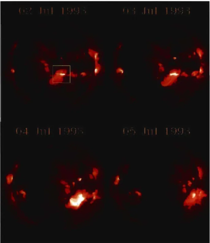
energies ranging between 1027 to 1033 ergs. In figure 1.4 we show a typical example of solar fiare as observed in X-rays. The sequence begins with the active region observed on July 2nd of 1993. The activity increases from July 3rd to 4th peaking on July 4th and decreases again on July 5th.

Flares are usually classified by their emissivity in different wavelengths. Two main classification schemes are generally used: the Ha importance and the soft X - ray

1.2. Solar Flares 18

Figure 1.3: Reproduction of a drawing by R.C. Carrington showing the location of the flare he observed while making a drawing of an active region [Carrington, 1859].

classification. The Ha-lines have the advantage of being formed in the visible region of the spectrum and of reacting strongly to the presence of a flare. They provide two pieces of information: the area covered by the flare, known as the importance or class of the flare (see classification on table (1.2)) and the strength of the Ha emission in the flaring region, known as the brightness. Flare brightness-scale is indicated by

f

faint; n normal and b brilliant. A flare covering 1000 millionth of the disk and with exceptionally bright Ha emission is a 3b - flare.

On the other hand X - ray classification is based on the integrated total output of soft X - rays detected in the wavelength range of 1 to 8

A.

With this information the strength of the flare is defined by the value of the peak intensity in units of power over length square as shown in figure 1.5. The most intense flares are the X-class. They can trigger planet-wide radio blackouts and long-lasting radiation storms, their intensity is 10-1 _{erg cm-}2 _{S-l, greater flares are designated by adding a number to the}

1.2. Solar Flares 19

Figure 1.4: A sequence of a fiaring region observed in X-rays by Yohhoh. http:j jwww.hao.ucar.edujPublicjeducationjslidesjslide15.html

1.2. Salar Flares 20 Area (*) Importance

<

100 S (su bfiare ) 100 - 250 1 250 - 600 2 600 - 1200 3

>

1200 4

Table 1.2: The importance classification of solar fiares (* in millionths of a solar hemisphere) .

GOES Xray

Flux (5 minute data)

:;

.

,

.

,

.

, ,

Solar Flares

:

~

X6 X2 /' 10-4~----~----~---__ ----~---__ :: -'l' -<:( o (JJ 1 X

~

IX) ff) K

W

B

10-5~

~

--~~~

~

__

--r--r~

~

~.~----~

~

--~

8

~

C <

~ 10-6~~--

~

--Mr

~

-~---+--

;-~~

-r·

#-

----~

~

----~

~

1 'B Li? o IX) A (f) L.LJ 10-8~~~~~~~~~~~~~~~.~~~~~~~~

g

Jul 12 Jul13 Jul 14 Jul 15

Universal Time

Up<lated 2000 Jul 14 19:04-:03 NOM/SEC Boulder, CO USA

Figure 1.5: Two X-class fiares and M-class detected by NOAA satellites in July 2000.

1.2. Solar Flares 21

letter X thus and X20 fiare has an inténsity of 2 erg cm-2 (20 times the intensity of

an X fiare). M-class fiares are medium-size with an intensity ten times smaller than X

fiares. The least intense fiares that can be observed but that have almost no infiuence on the Earth environment are C and B fiares. Their intensities are 10-3 _{erg cm-}2

and 10-4 _{erg cm -2 S-1 respectively.}

From figure 1.5 it is apparent that in fiare phenomena we can identify two different stages: the rising phase and the thermalization phase. The former is characterized by a rapid (couple of seconds) increase of energy while in the latter, energy decreases with a smoother slope that can last hundreds of seconds.

When analyzing many hundred of thousands of recorded fiares observers found that the frequency distribution of the energy released by fiares had the form of a tight power law, spanning at least eight orders of magnitude in fiare energy [Aschwanden et al., 2000]. Specifically, if

f

(E) dE is the fraction of fiares releasing an amount of energy between

E and E

+

dE per unit of time the frequency distribution takes the form:

(1.1)

with a

>

O. This power-Iaw is indieative of the absence of a typical scale for the

relea~ing of energy meaning that the system behaves in a self-similar way.

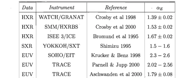
In table (1.3) we present recent determinations of fiare power-Iaw indices for the energy release. Translating the observed fiare X-ray or EUV fiuxes to volumetrie energy release is a very complex task that involves many assumptions such as: the geometrical shape of the fiaring region, the physical conditions within the fiare vol-ume and the mechanism responsible for the emission of hard radiation (for more de-tails in [Lee et al, 1993]). In fact the definition of what is to be considered a fiare depends strongly on the detection threshold and the temporal and spatial limits im-posed by detection instruments (a complete discussion on the subject can be found in [Aschwanden et aL, 2000]). In these observational and data analysis difficulties lies the

1.2. Solar Flares 22

Figure 1.6: X28 fiare in EIT 195 filter observed on 4th November 2003. It satu-rated the X - ray detector aboard NOAA's GOES satellite that monitors the Sun http:j jsohowww.nascom.nasa.govj.

1.3. A simple model of solar flares 23

Data Instrument Reference - ŒE

HXR WATCH/GRANAT Crosby et al 1998 1.39

±

0.02 HXR SMM/HXRBS Crosby et al 2000 1.53

±

0.02 HXR ISEE 3/ICE Bromund et al 1995 1.67

±

0.02

SXR YOKKOH/SXT Shimizu 1995 1.5 - 1.6

EUV SOHO/EIT Krucker & Benz 1998 2.3 - 2.6 EUV TRACE Parnell & Jupp 2000 2.02 - 2.56 EUV TRACE Aschwanden et al 2000 1.79

±

0.08

Table 1.3: Observational determinations of flare power-Iaw indices for the energy release.

reason for the significantly variation between the power-Iaw indices reported in table (1.3) even when in sorne cases the same instruments have been used.

In order to understand and predict solar flares many models have arisen, each of them featuring different characteristics. Nevertheless, there is universal agreement on the fact that the magnetic fields is the main ingredient and plays a crucial role both as an energy source and as a trigger mechanism. In the following section, we present a standard model of solar flares that takes this fact into account.

1.3 A simple model of solar flares

The magnetic structure of the magnetic field around sunspots is the key concept when modeling the occurrence of flares. Flares almost always occur in active regions which, in their simplest form, are bipolar magnetic structures, consisting of adjacent patches of outwardly and inwardly oriented magnetic field, as shown in figure 1.7. To de-scribe a magnetized plasma like the one existing in the coronal environment we use

1.3. A simple model of solar Bares 24

Figure 1.7: Ultraviolet-light image of coronal loops. Large arcs of gas and energetic particles confined by the magnetic field that make up the solar corona are seen by the the TRACE satellite telescope.

1.3. A simple model of solar flares 25

the magnetohydrodynamic (MHD) equations. The MHD approximation embodies the conservations principles derived from the equations of fiuid dynamics and electromag-netism.

If p is the mass density of the magnetic fiuid and v is the fiow field the mass conservation equation takes the form:

ap

&t -

v . V' P = -pV' . v. (1.2)

In the incompressible case, equation (1.2) can be written as: V'. v =0.

The Navier Stokes equation that expresses the momentum conservation is:

av

1 1 2

-

+

(v· V')v = -(V' x B) x B - -V'p

+

vV' v

at·

4np p (1.3)

where B is the magnetic field, P is the fiuid pressure and v is the kinematic viscosity. The magnetic field is related to the current density and electric field by Ohm's law which, for the case of a neutral nonrelativistic fiuid, takes the simplified form:

a(E

+

~

x B)

=

j ,

c (1.4)

where a is the electrical conductivity of the plasma. The current j is related to the magnetic fields by Ampère's law:

'\7 B 4n.

v x = - )

c

where we have neglected the displacement current:

(l/c)a

t

E.

Substituting equation (1.4) into Faraday's equation:

aB

-

_at

= -cV' xE

_.

(1.5)

1.3. A simple model of solar flares 26

we can obtain the induction equation which gives the evolution of the magnetic field:

aB

c2

-a

= \7

x

(v

x

B)

+

- 4 \72 B .

t na (1.7)

The set of equations is completed with the solenoidal condition for the magnetic field:

\7 . B

=

O. Equation (1.7) isknown as the induction equation. The first term on the right hand side describes the advection of field lines by the fluid, while the second term is the diffusive term.

The ratio of these terms for a typical length sc ale L and a velo city scale v is the m~gnetic Reynolds number:

Rm

= Lv ,

Tl

with Tl

=

c2/ (4na) the magnetic diffusivity.

(1.8)

The fact that equation (1. 7) is highly non-linear makes it difficult to extract immedi-ate consequences for the behavior of the magnetic field; nevertheless, sorne conclusions may be derived when studying two extreme cases:

Rm

»

1 and

Rm

«

1. In the case of a high conductivity fluid (a ---+ (0), there is no diffusion and the induction equation

takes the form:

aB

ât

=

\7 x (v x B) . (1.9)

Equation (1.9) expresses the conservation of the magnetic flux that go es through any closed curve that moves with velocity v [Priest, 1982]. Thus, the magne tic field moves with the fluid. This result is the magnetic analogy of the Kelvin's theorem of vorticity, which states that, for an inviscid flow, vortex lines move with the fiuid. If

Rm

«

1 then the advective term is negligible and the induction equation becomes a diffusion equation. In this case the typical timescale for the diffusion of magnetic field is:

1.3. A simple model of solar fIares 27

To explore this deeply let's consider the simple case presented by [Priest

&

Forbes, 2000]. For a one-dimensional magnetic field B(x, t)y satisfying:

(1.11)

the solution for this equation is:

B(x, t) =

J

_{G(x - x', t)B(x' , O)dx'} (1.12)

where B(x,O) is some initial condition and.G is the Green function:

G(x X , ,

t)

=

~

1 exp [ .

-(x -

411

t

X')2

].

(1.13) If we assume that initially we have an infinitesimally thin current sheet as shown in figure 1.8: B

=

Bo for x

>

0 and B

= -

Bo for x

<

O. We expect that the steep magnetic gradient will spread out as the magnetic field evolves in time. The solution of equation (1.11) can be written in terms of the error function:

B(x,

t)

₍_x_) _

_~

- . t;:;; 2 BOlx/v'4rit e _u2 du .

Y~11t yn

°

.

(1.14)

According to this expression, the magnetic field diffuses away in time at a speed 11/ l where l is the width of the sheet and is of the order of."fiit. The resulting magnetic field strength at a fixed value of x decreases with time so the field is annihilated as we show in figure 1.9.

It is worth calculating the evolution of magnetic energy:

a

JOO

B2

Joo

B aB

- dx = dx

at -00 8n -00 4n at

(1.15)

substituting then expression for ~~ with equation (1.11) and integrating by parts we firid:

1.3. A simple model of solar flares 28 Ba - _{: ....}

_-

-

-....

-t=t

,

,-.... ,-/ / / - 1 t=o 1 1 _t=t 1 2 1 1 1. _{VT}t, VT}t} 2 1 : 1 1 1 1 1 :-/ / / ,-.... ....

- -

-

-

. ... Ba

Figure 1.8: The magnetic field as a function of distance in a one-dimensional sheet that is diffusing from one of initially zero thickness. Three different consecutive times are plotted (t = O,t = tl and t = t2 ).

1.3. A simple mode} of solar Bares 29 t .1 1

•

Î: 1

•

t=.O

~'. i: I-I 1 1

•

1

•

t=1.:z

•

,

•

•

l;.

,

1

•

,

t=,t

₂

Figure 1.9: Annihilation of magnetic field Hnes (Figure 3.2 in [Priest

&

Forbes, 2000]).

1.4. Reconnection 30

The first term on the right side vanished because ~~ = 0 at infinity and, remembering that for this example the current is j = 4c" ~~, we obtain:

a

1

00

fJt -00 B (1.17)

this means that an the magnetic energy is transformed into heat by ohmic dissipa-tion. Under normal coronal conditions the dissipation timescale Td is of the order or

1010_-16 _{sec which is many orders of magnitude longer than the onset and}

thermaliza-tion times for flares. The former is typically 1 - 2 sec and the latter is of the order of 100 sec (as shown in figure 1. 5).

Magnetic reconnection is the most plausible mechanism to obtain timescales in ac-cordance with the rapid release of energy in the solar corona. The following section is devoted to a presentation of the basic theory regarding this process.

1.4 Magnetic Reconnection

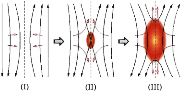
Magnetic reconnection is a fundamentaI physical pro cess occurring in a magnetized plasma and is probably the most promising one for explaining large-scale, dynamic releases of magnetic energy. During the reconnection process, magnetic field Hnes break and rearrange in a lower energy state. The excess magnetic energy is converted into kinetic energy and heat, and large electric currènts and electric field are created. Figure 1.10 shows a simple scheme of the reconnection process: magnetic field lines of opposite polarities are brought together. As this takes place the value of the magnetic gradient in the central region increases and produces a strong current along a diffusion region called CUITent sheet and perpendicular to the field lines .. Within this region field lines are broken and reconnected producing a new magnetic topology. This process may go on as fresh magnetic fields are brought into the diffusion region.

1.4. Magnetic Reconnection 31

(1)

(I1)

(III)

Figure 1.10: Three stages in the reconnection process. (1) Driven field lines ap-proaching. (II) A diffusion region is formed. A strong current perpendicular to the plane of the paper appears. Field lines broke and reconnect. (III) New connectiv-ity between field lines. Magnetic energy is converted into kinetic and thermal energy http:j jwww.aldebaran.czjastrofyzikajplazmajreconnectionj.

1.4. Magnetic Reconnection )

t

ln (

("" - - - "" - - '- - -, 2L '-.:.. - "" - ...;.. - - - - ..:.. -

~

.... v .

,. ,out Bout 32

Figure 1.11: Sweet-Parker model. The diffusion region is shaded. PI,asma velocity is indicated by thick-headed arrows and the magnetic field lines by thin-headed arrows (Figure 4.2 in [Priest & Forbes, 2000])

One of the most important questions to de ci de if reconnection is or is not the mech-anism responsible of e!lergy release in solar fiares has to do with the typical timescales dominating the process. To begin this discussion we present the simplest model of magnetic reconhection.

1.4.1

Sweet-Parker Mechanism

The Sweet-Parker model assumes that reconnection takes place in a thin regiori known as the diffusion region. The main goal of this model is to describe the magnetized fiuid by me ans of the the magnetohydrodynamic equations (MHD) and to estimate the value of each term in the steady state in order to obtain the typical rate of reconnection of magnetic field lines ..

1.4. Magnetic Reconnection 33

In a 2D-steady state the electric field is uniform within the difussion region, so Ohm's law takes the form:

1 .

Eex-J.

0-Outside this region the current is zero so:

(1.18)

(1.19)

where Vin and Bin are the velocity and magnetic fields entering the diffusion region. In

this system Ampère's law takes the form:

(1.20)

Eliminating E between equations (1.18) and (1.19) and combining the result with equa-tion (1.20) we can obtain the velocity at the entrance of the diffusion zone as a funcequa-tion of the width of the current sheet:

(1.21)

Assuming that the reconnection of lines is steady then conservation of mass implies that the rate at which the mass is entering the sheet is the same as the going-out rate, so that:

LVin ex 8 Vaut, (1.22)

where Lis the length of the diffusion zone (see figure 1.11). Eliminating the width (8) using equation (1.21) and (1.22) we obtain:

1.4. Magnetic Reconnection 34

and the flux conservation condition gives:

(1.24)

The relation between the velocity and the magnetic fields can ?e obtained combining equations (1.23) and (1.24):

(1.25)

and with this relation we can estimate the value of t~e current j rv Bin/8 so that

Lorentz 's force along the current' sheet is:

( _J .

_x

_B ) x ex: J , B out ex: BinBout 8 (1.26)

This force accelerates the plasma from rest at the neutral point to Vout. Replacing this

into "Navier-Stokes" equation we have:

(1.27)

Eliminating Bout with equation (1.25) and (1.27) we obtain:

Bin

Vout ex: )47fp = Va (1.28)

where Va is the Alfvén's speed. Thus the magnetic force accelerates the plasma to the

Alfvén's speed.

The dimensionless reconnection rate (M) is defined as the ratio between the incom-ing and the outgoincom-ing flux:

M = Vin.

Vout

1.4. Magnetic Reconnection 35

Considering equation (1.29) as the reconnection rate has led to sorne confusion, since properly speaking the reconnection rate is the rate of flux change at the neutral point but in steady conditions M is conventionally used as a measure of the reconnection rate. Dividing the square root of equation (1.23) by Vaut (which is equal to Va by equation

(1.28)) we can obtain an expression for the reconnection rate:

(1.30)

where

Rm

is the Reynolds magnetic number, that can be written in terms of the mag-netic diffusivity:

(1.31 )

In the solar outer atmosphere Reynolds magnetic number has typical values between 108 _{and 10}14_{; this yields typical reconnection timescales which are 1/}

_yi

_Rm

_{smaller than}

dissipation timescale in the corona. The Sweet-Parker reconnection timescaie is still far from eruptive flare phenomena. In an attempt to give an answer to this question in 1983 E. N. Parker proposed a collective reconnection effect occurring in the corona: nanoflares.

1.4.2

Coronal heating and Parker's conjecture

Regardless of the many open questions that magnetic reconnection theory still poses, there is no doubt that, when reconnection occurs, most of the energy liberated by the process ends up heating the plasma surrounding the flaring site as the charged particles, accelerated by the electrical field produced during reconnection, thermalize with the surrounding cooler plasma.

1.4. Magnetic Reconnection 36

Given the flare frequency distribution f(E) (see equation (3.1)), the total energy per unit time released collectively by an ensemble of solar flares is:

dET

=

fEmax f(E) EdE

=

fo

[E~-a

1

Emax

dt } Emin 2 a E .

mm

for a

=J

0 . (1.32)

If a = 2 the total energy is:

ET - fo log (Emax/ Emin) . (1.33)

The values of fo and Emax have already been estimated (see [van Ballegooijen, 1986]). They are insufficient to provide a total flux of the order of 107 _erg/cm2_{/s even at the}

solar maximum. This implies that, if the largest flares are to be responsible for coronal heating, then a

<

2; on the contrary if a

>

2, the smallest flares dominate the energy release. Parker has conjectured theoretically that these 'nanoflares' are responsible for coronal heating.

In Parker's conception the magnetic free energy is stored in the corona. Stochas-tic movements of the photospheric fluid do move around the footpoints of magneStochas-tic coronalloops as shown in figure 1.12. Because the coronal plasma is highly conductive the frozen-in condition for the magnetic field holds up resulting in a complex, entan-gled magnetic field force free almost everywhere except in many small electrical currents sheets which form spontaneously in highly-stressed regions (current sheets). As the cur-rent in these sheets goes beyond sorne threshold, reconnection takes place and magnetic energy is released.

If Parker's model is correct then a should be greater than two. In order to comple-ment observational analysis a theoretical calculation of a appeared necessary. There have been attempts to solve numerically the MHD equations that describe Parker's sce-nario (see for example; [Galsgaard, 1996], [Mikic et al., 1989], [Longcope & Sudan, 1994]). Those simulations could not reach a parameter regime where all scales were resolved,

1.4. Magnetic Reconnection 37

/z=L

/ t

~-_.-

-

.-"

~

/ "" ,," ~, t' -) ;' , "

,-L_" ___

'_~_

..

_~_~_""'

___

-;._~_'f,,_"'

__

"S_lII._,_.::::::::_~_/_"

___

~_"

';';:" -...

Z

=

0

Figure 1.12: A sketch of the idealized situation of the uniform magnetic field that conforms a coronal loop. The magnetic structure has been straightened and extends between the two extremes z

=

0 to z

=

L located at the photosphere through the highly conducting fiuid that forms the solar corona. The field is fixed at z = L while the footpoint (z = 0) is driven randomly among its neighbors by photospheric turbulent convective motions, leading to the formation of current sheets. (extracted from Figure 11.2 in [Parker, 1979])

1.5. Self-Organized Cri ticali t y and Flares 38

and thus could not obtain reliable probability distribution functions with which to es-timate a. Self-organized criticality came along as a shortcut towards this goal.

1.5

Self-Organized Criticality and Flares

Self-organized criticality (SOC) has been proposed in the late eighties by Bak, Tang and Wiesenfeld [Bak, Tang & Wiesenfeld, 1988] as a general framework to understand the occurrence of power laws in nature. The basic idea of their model is that dynamical systems with many spatial degrees of freedom can, under certain circumstances, evolve into a self-organized critical state. The prototypical SOC model is the so-called sandpile model.

1.5.1

The sandpile system

Consider a circular table on which sand grains are dropped one at a time. The grains might be added at random positions or only at one point. This process can cause local disturbances but there is no obvious direct communication between grains that are far apart in the pile. Eventually, the sand dropping willlead to the buildup of a more or less conical pile as shown in figure 1.13. The sand pile steepens until its slope reaches a critical angle: the angle of repose beyond which further addition of sand leads to an

avalanche, thus sand is swept down so that the slope remains close to its critical value. The addition of grains of sand has transformed the system from a state in which the individu al grains follow their own local dynamics to a critical state where the emergent dynamics are global. At this point thesandpile is in a statistically stationary state, with the average rate of sand falling off the table's edge equal to the rate in which sand grains are supplied. But it is a dynamical stationary state in which relaxation is related

1.5. Self-Organized Criticality and Plates 39

."

.,.

Figure 1.13: Cartoon sandpile (adapted from Figure 1 in [Bak, 1996]).

to the occurrence of occasional avalanches that may span the whole pile. This means that a newly dropped grain can affect another sand grain located &nywhere throughout the pile by triggering the avalanche so the system is in a critical state.

The sand pile is an open dynamical system. It has many degrees of freedom: the number of grains of sand. One of those grains landing on the pile represents the addition of potential energy. When the sand moves along the slope this energy is transformed into kinetic energy. Once the grain reaches an equilibrium the kinetic energy is trans-formed into heat. The critical state is maintained by the external addition of sand. A typical feature of this kind of systems is that the energy input is slow and steady while the energy release is strongly intermittent. The sandpile is only an example of the critical behavior of different, phenomena. In the next section we resume the main characteristics of self-organized critical systems.

1.5. Self-Organized Criticality and Flares 40

1.5.2 Self-Organized Critical State

The central aspects of self-organized critical systems can be found by understanding the meaning beneath each word. A self-organized system naturally evolves to astate without detailed specification of the initial conditions or external control during evolu-tion. A self-organized state is said to be critical when although the interaction between the elements of the system is local, the emergent property of this interaction is global. It does not matter how two elements of the system interact as long as this interaction is local and allows the definition of a threshold. It is in this sense that the critical state is said to be an attractor of the dynamics. Thus, if the driving rate is suddenly increased, large avalanches will appear and they will rapidly remove the surplus of sand from the system. On the other hand if one artificially removes sand from the pile, the frequency of large, boundary-discharging avalanches will go down until the angle of repose has been restored throughout the pile. Another important feature in order to obtain an interaction-dominated system is the driving rate. Strong driving will not allow the system to relax from one metastable configuration to the other. Finally, a universal characteristic of physical systems in a SOC state is that energy is dissipated in all length scales. Once the critical state is reached the system stays there and it is possible to characterize the behavior of the system by a number of critical exponents.

Self-organized criticality of interacting systems is often studied using cellular au-tomata models. A cellular automaton (CA) consists of a discrete dynamical system with many degrees of freedom. Space, time, and the states of the system are dis-cretized. Each element of the system evolves according sorne set of discrete local rules. In 1991 Lu and Hamilton [Lu & Hamilton, 1991] proposed that the solar coronal mag-netic field is in a self-organized critical state and presented the first CA model for solar flares. Since then several CA for solar flares haven been proposed. Although different in many aspects all of these models share common features with Lu and Hamilton's model. For this reason we present in the next section a basic lattice model adapted

1.6. A basic lattice model 41

::

.

Figure 1.14: A two-dimensional regular cartesian lattice. A field quantity B is de-fined at each node

(j,

k). Four nearest neighbors are red-dotted. (see Figure 1 in [Charbonneau et al., 2001])

from [Lu et al., 1993] and examine the physical interpretations and limitations of the lattice model.

1.6 A basic lattice model

1.6.1

The lattice and the driving mechanism

On a simple regular 2D-cartesian lattice it is possible ta define a physical quantity Bk

on each lattice node. This quantity is and assumed ta be a continuous, scalar variable (see figure 1.6.1).

1.6. A basic lattice model 42

and

Ba

gives the magnetic energy, so the lattice energy (El) is:

EI=LB~, (1.34)

k

and the lattice me an magnetic field

<

B

>

is:

(1.35)

where N and D are the size and dimension of the lattice.

The existence of a globally stationary state requires that the physical quantity de-fined on the lattice be externally driven. The simplest way to do this is to add a succession of perturbations bB at randomly selected interior nodes. This occurs only when the system is not avalanching. In or der to ensure a SOC state to be attained the driving must be weak and the relation between bB and

<

B> should be:

IbBI

«1.

<B> (1.36)

Once the perturbation pro cess has started each node has to be tested for stability.

1.6.2

The stability criterion

The stability criterion is based on the curvature of the magnetic field (!:lB), defined as: 1

!:lB = Bk - -

L

Bk ,

2 D nn=l

(1.37)

where the sum runs over the two-dimensional nearest neighbors "n, n" on the lattice. The configuration is defined to be unstable when

I!:lBI

>

Be. Be is a critical value that must remain non-zero. The idea of measuring the curvature of the magnetic field was originally developed by Lu & Hamilton [Lu & Hamilton, 1991]. Up to that point most models used a height-triggered or slope-based stability criteria.

1.6. A basic lattice model 43

In Lu & Hamilton's conception, Ô.B is a gradient but actually it has ,the form of a second-order centered finite difference expression for a D-dimensional Laplacian operator as shown in [Galsgaard, 1996]. AlI models with this kind of stability criterion are referred to in the literature as 'curvature-triggered' systems.

1.6.3

The redistribution rule

If ÔB exceeds the critical value some action is needed to restore stability, A natural procedure is to decrease B at the unstable node and distribute the excess at neighboring nodes. 80 the new magnetic field at the unstable node is:

(1.38)

and at the neighboring nodes is:

2D

Bnn ----> Bnn

+

2 D

+

1 Be . (1.39)

After the redistribution has been applied as prescribed by equation (1.39), it is possible that one or more nearest-neighbor nodes might have become also unstable; if this is the case, the redistribution rule is to be applied on those nodes and so on until stability is restored everywhere. The redistribution rule presented in (1.39) is locally conservative, meaning that Bk

+

I:

Bnn remains constant but the total energy of the lattice is reduced. The discrete energy lost is:

e

r =

2

D

(21

ÔB

1 _

1) B2 .

2D

+

1 Be e (1.40)

From this expression one can de duce that the smallestenergy that can be released by a single node that has infinitesimally exceeded the threshold value Be is:

2D 2

1.6. A basic lattice model 43

In Lu & Hamilton's conception, !:lBis a gradient but actually it has the form of a second-order centered finite difference expression for a D-dimensional Laplacian operator as shown in [Galsgaard, 1996]. All models with this kind of stability criterion are referred to in the literature as 'curvature-triggered' systems.

1.6.3

The redistribution rule

If !:lB exceeds the critical value some action is needed to restore stability. A natural procedure is to decrease B at the unstable node and distribute the excess at neighboring nodes. 80 the new magnetic field at the unstable node is:

(1.38)

and at the neighboring nodes is:

2D

Bnn ---+ Bnn

+

2

D

+

1 Be . (1.39)

After the redistribution has been applied as prescribed by equation (1.39), it is possible that one or more nearest-neighbor nodes might have become also unstable; if this is the case, the redistribution rule is to be applied on those nodes and s6 on until stability is restored everywhere. The redistribution rule presented in (1.39) is locally conservative, meaning that Bk

+

E

Bnn remains constant but the total energy of the lattice is reduced. The discrete energy lost is:

= 2 D ( j!:lBI _ I)B2

er _{2 D}

+

_{1 2 Be e •} (1.40)

From this expression one can de duce that the smallest energy that can be released by a single node that has infinitesimally exceeded the threshold value Be is:

1.7. Physical Interpretation 44

. The total energy release after one iteration will be:

(1.42)

with the sum extending over aU the nodes that have been unstable during the corre-sponding iteration. Regardless the details of the energy input method aU SOC models of solar fiares have one important thing in common: energy injection is slow and steady whereas energy release is strongly intermittent, mimicking in this way the classical sandpile.

Since 1991, many SOC models for solar fiares have been constructed using different kind of lattices, varying the stability criteria or the redistribution rule. Many of them have successfuUy calculated power-law indices that remain close the one observed in solar fiares. In table (1.4) we show (just as an example) sorne of the power-law indices obtained for total energy for several SOC models available in theliterature. Slight differences betweeri the models are related to the different manners each group went about carrying out the fits. From table (1.4) we note that there are not great differences between 2 D and 3 D models and the a indices faU nicely within the ranges set by the observational inferences (see table (1.3)).

1.7 Physical Interpretation \

Up to this point we have described aU the elements that are included in most classical SOC models for solar fiares. Now we head forward to discuss the physical meaning of each of those elements.

The most straightforward physical association ofthe nodal field Bk is to the magnetic field B, in which case equation (1.35) for lattice energy makes sense. However in general this leads to V' . B

=f

O. Associating Bk with a vector potential A such that B

=

V' x A

1.7. Physical Interpretation 45

Reference Geometrie Model ND

(*)

CiE

Lu et al. 1993 503 _1.51

Lu & Hamilton 1991 303 _1.4

Charbonneau et al 2001 10242 _1.421

1283 _1.485

Longcope & N oonan 3002 1.34

Zirker & Cleveland 322 _1.45

Table 1.4: Power-Iaw indices for total energy (E).

(*)

N is the size of the lattice and D is the dimensionality of the model.

solves the problem of the conservation of the magnetic flux but also offers a plausible interpretation of the driving process. Adding an increment 8A to the lattice can be thought of as a twisting of the magnetic field. The problem with this interpretation is that

l:

B~ is no longer a measure of the magnetic energy and jeopardizes the whole ide a of comparing model time series to flare observations. The re-interpretation of Bk as the vector potential provides a physically meaningful interpretation for the instability threshold. It can be noted here that equation (1.37) has the form of a finite difference expression for the Laplacian operator, so the threshold condition implies that magnetic reconnection takes place when V2 _{A exceeds certain value.}

Remembering that B = V x A, Ampère's law (equation 1.5) takes the form:

j

=

~V

x

(V

x

A)

=

~[-V2A+V(V

.A)] .

4n 4n (1.43)

Using the Coulomb Gauge (V· A = 0), equation (1.43) leads us to: