HAL Id: hal-00287425
https://hal.archives-ouvertes.fr/hal-00287425
Submitted on 11 Jun 2008HAL is a multi-disciplinary open access
archive for the deposit and dissemination of sci-entific research documents, whether they are pub-lished or not. The documents may come from
L’archive ouverte pluridisciplinaire HAL, est destinée au dépôt et à la diffusion de documents scientifiques de niveau recherche, publiés ou non, émanant des établissements d’enseignement et de
Objective quality assessment of color images based on a
generic perceptual reduced reference
Mathieu Carnec, Patrick Le Callet, Dominique Barba
To cite this version:
Mathieu Carnec, Patrick Le Callet, Dominique Barba. Objective quality assessment of color images based on a generic perceptual reduced reference. Signal Processing: Image Communication, Elsevier, 2008, 23 (4), pp.239-256. �10.1016/j.image.2008.02.003�. �hal-00287425�
Objective quality assessment of color images
based on a generic perceptual reduced
reference
Mathieu CARNEC, Patrick LE CALLET and Dominique BARBA
IRCCyN, ´Ecole Polytechnique de l’Universit´e de Nantes, Rue Christian Pauc, La Chantrerie, NANTES, France
Abstract
When an image is supposed to have been transformed by a process like image enhancement or lossy image compression for storing or transmission, it is often necessary to measure the quality of the distorted image. This can be achieved using an image processing method called “quality criterion”. Such a process must produce objective quality scores in close relationship with subjective quality scores given by human observers during subjective quality assessment tests.
In this paper, an image quality criterion is proposed. This criterion, called C4, is fully generic (i.e., not designed for predefined distortion types or for particular images types) and based on a rather elaborate model of the human visual sys-tem (HVS). This model describes the organization and operation of many stages of vision, from the eye to the ventral and dorsal pathways in the visual cortex. The novelty of this quality criterion relies on the extraction, from an image rep-resented in a perceptual space, of visual features that can be compared to those used by the HVS. Then a similarity metric computes the objective quality score of a distorted image by comparing the features extracted from this image to features extracted from its reference image (i.e., not distorted). Results show a high correla-tion between produced objective quality scores and subjective ones, even for images that have been distorted through several different distortion processes. To illus-trate these performances, they have been computed using three different databases that employed different contents, distortions type, displays, viewing conditions and subjective protocols. The features extracted from the reference image constitute a reduced reference which, in a transmission context with data compression, can be computed at the sender side and transmitted in addition to the compressed image data so that the quality of the decompressed image can be objectively assessed at the receiver side. More, the size of the reduced reference is flexible. This work has been integrated into freely available applications in order to formulate a practical alternative to the PSNR criterion which is still too often used despite its low cor-relation with human judgments. These applications also enable quality assessment for image transmission purposes.
Key words: Image quality, image quality assessment, reduced reference, human visual system, visual perception
1 Introduction : Image quality criteria
Image quality assessment presents an important interest for image services that target human observers. Indeed, measuring image quality enables to ad-just the parameters of image processing techniques in order to maximize image quality or to reach a given quality. Image quality can be measured in two dif-ferent ways. The first, called “subjective quality assessment”, consists of the use of human observers who should score image quality during experiments called “quality assessment tests”. The second one is called “objective quality assessment”. It consists of the use of a computational method called “quality criterion” which produces values that score image quality. One of the proper-ties required for an image quality criterion is that it should produce objective scores well correlated with subjective quality scores produced by human ob-servers during quality assessment tests. From a practical point of view, such a criterion is an algorithm able to score (on a scale) the quality of a tested image which may have been distorted. While computing quality scores can be a simple task, producing meaningful visual quality scores, which means scores well correlated with subjective quality scores given by human observers, is much more complicated and corresponds to much more complex tasks.
Many quality criteria have been proposed in the past and are well described in literature. They can be roughly divided into three main categories : Full Ref-erence (FR) criteria, Reduced RefRef-erence (RR) criteria and No RefRef-erence (NR) criteria. Obviously, all these criteria are a function of the distorted image. FR criteria are also a function of the original image which is assumed to be free from distortions (called the “reference image”). RR criteria require a partial knowledge of the reference image (this knowledge is called the “reduced ref-erence”). At last, NR criteria don’t have any information about the reference image. Some recent quality assessment techniques can hardly be classified in these three categories, for example when image quality is computed from a watermark distortion [1]. For RR criteria, it is difficult to choose the types of features which are the most useful to describe image quality and to efficiently exploit these features. Finally, it is difficult for NR criteria without any infor-mation on the reference image to distinguish which part of the image signal is due to distortions and which part is due to the reference image.
Other differences come from the fact that existing criteria use various tech-niques. Some criteria first compute a map of distortions [2] - this is only really possible for FR criteria - whereas the others quantify by a parameter the
im-portance of each distortion type, depending on the distortion process (like the blocking effect in JPEG image coding for example [3]). Moreover, some criteria include a model of the Human Visual System (HVS), for example to locally balance visual distortions [4], whereas others more directly use the im-age signal [5].
FR criteria are evidently considered as the best way to get good performances in quality assessment. But they cannot be used in applications where the original image is not available or, as in a transmission context with lossy com-pression, cannot be evidently transmitted with the compressed image data. At this level, the problem with the criteria used in transmission contexts (RR or NR) is that most of them are designed for a limited number of predefined distortion types (lack of genericity). Moreover, most criteria are not used be-cause they are not easily available as a software (and therefore need to be implemented) or because they require too complex computations for the tar-geted application. These are the main reasons why the simple PSNR criterion (which is a FR criterion) is still too often used as its implementation is quite easy and its complexity is very low.
To solve these problems, the image quality criterion proposed in this paper is fully based on a model of the HVS and does not depend on predefined dis-tortion types. However, the complexity problem still remains since the HVS model (which is an essential part of the proposed image quality criterion) still requires a lot of computations.
This paper is organized as follows. At first, the different existing approaches to design RR criteria and the choices that have guided the design of the criterion described in this paper are presented in section 2. Section 3 introduces the HVS model to be used here. The implementation of this HVS model is explained in section 4. This implementation leads to the building of image descriptions which are used to assess image quality, as detailed in Section 5. Eventually, the image quality criterion performances is presented in section 6 on three different images bases that were realized using different contents, distortions type, displays, viewing conditions and subjective protocols.
2 Reduced Reference (RR) criteria
Reduced Reference (RR) criteria use short descriptions of the reference and distorted images to produce an objective quality score of the distorted image. The reduced description (RD) of the reference image is called “reduced ref-erence” (RR). Each RD is a set of data (the “features”) computed from the image. In a practical context of image quality assessment, within an image
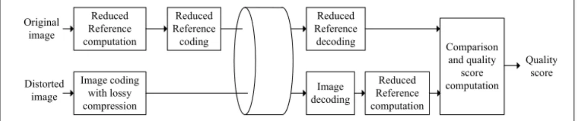
transmission service, the RR must be coded and transmitted with the com-pressed image data produced by the coder. Contrary to the transmission of the compressed image, the transmission of the RR is done assuming that there is a side channel with no transmission error to transmit the RR while the se-quence is transmitted through a higher bandwidth channel. The assumption of a side channel without error is realistic as long as the RR represents a limited bandwidth and so can be quite easily protected against transmission errors. Once coded, the RR must correspond to a reasonable bit budget in or-der not to increase too much the amount of data to transmit. At the receiver end, one extracts the RR and compares it to the RD computed on the de-coded image. From this comparison one produces an objective quality score of the distorted image. The deployment of a RR criterion is described in figure 1.
Reduced Reference computation Reduced Reference coding Original image Distorted image Quality score Comparison and quality score computation Reduced Reference computation Reduced Reference decoding Image coding with lossy compression Image decoding
Fig. 1. Block diagram of a RR image quality criterion
In literature, few RR criteria can be found. They can be roughly divided in two groups according to the type of features used in the RD. The first group gath-ers RR criteria which use features describing the image content. For example, Voran and Wolf from the ITS (“Institute for Telecommunication Science”) developed a RR video quality criterion [6] in 1992, based on three features that describe the image spectrum. The ITS has also developed a RR video criterion [7] which was included in an ANSI standard [8] in 1996. This latter criterion also uses three features. The first feature describes the high spatial frequencies. The two other features inform on the temporal activity between two successive images. By comparing the features computed from a reference frame of a video with the same features computed from the distorted frame of this video, a quality score of the distorted frame is produced. Then all the computed frame quality scores are combined to produce a unique video quality score. In this criterion, all the features are computed rather directly from the raw image data. Wang and Simoncelli [9] have also designed and developed a RR image quality criterion based on features which describe the histograms of wavelet coefficients. Two parameters describe the distribution of the refer-ence image wavelet coefficients using a Generalized Gaussian Density (GGD) model. These two parameters constitute the RR. At the receiver end, the dis-tribution of wavelet coeffients is computed from the distorted image and is compared to the distribution of the reference image to produce the quality
score of the distorted image. The criteria of this first group can theoretically be used with a wide range of distortion types since their RR is content-oriented and not designed for predefined distortion types.
The second group of RR criteria contains those which use a set of distortion-based features, each of them measuring the importance of predefined dis-tortions. For example, Kusuma introduced [10] a RR criterion called HIQM (“Hybrid Image Quality Metric”) based on features describing the importance of blocking effect and of blurring effect respectively. Some other features ex-press the importance of aliasing effects, contrast reduction and block loss (due to packet loss during transmission). In HIQM, the importance of blocking ef-fect is computed using Wang’s method [11] and the importance of blurring is measured by Mariziliano’s method [12]. Aliasing effects and block loss are detected by Saha and Vemuri’s method [13]. Contrast reduction is measured using an original method, based on image histogram. The quality score is built using a balanced sum of the importances of each distortion type. This crite-rion could be a NR critecrite-rion but the HIQM value depends on image energy so that the HIQM value of the reference image must be known in order to detect distortions and therefore this HIQM value constitutes the RR. The criteria from this second group are not generic since the RR is distortion oriented. Considering these two kinds of approaches, the work presented in this paper concentrates on the design and integration of an elaborate HVS model in a RR criterion. Roughly speaking, the latter is based on fully perceptual features, independent from distortion types, extracted at psychophysically important locations. This fills up the gap between FR criteria, for which HVS models have permitted to increase performances, and RR criteria which are based on features more directly extracted from the raw image data. This approach is based on the hypothesis that human assessment of image quality is performed by estimating the importance of annoyance which corresponds to the difficulty one has in recognizing objects in images. Therefore by simulating the HVS behavior, the extracted information is that which is relevant for perception and so, for pattern recognition when humans look at the image content.
3 Human Visual System Model
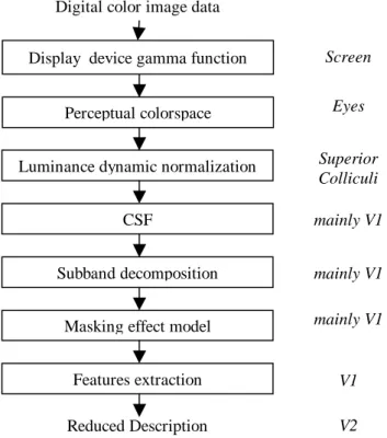
In order to develop a human vision based RR criterion, a rather elaborate model of the HVS has been set up. The full model has been extensively de-scribed in [14] and [15]. This model has been established from neurophysiology publications [16–19]. Only a subset of this full model will be implemented here so only the useful part of the latter is described in figure 2. It takes into ac-count the eyes, V1 and V2 areas and the ventral pathway.
The eyes are the starting point of the diagram presented in figure 2. Both contain a sensitive layer at the back: the retina. In the retina, cones and rods convert the light into bioelectrical signals. The domain of interest of this work deals with the photopic vision (day vision). Since rods serve for night vision, only cones will be of interest in this paper. There are 3 types : L (565 nm, red), M (535 nm, green) and S (430 nm, yellow-green). Between the cones and the optic nerve, a succession of cells organized in layers is crossed by bioelectrical signals : horizontal cells, bipolar cells, amacrine and ganglion cells. In each eye, ganglion cells’ axons form the optic nerve [20]. Fibers of each optic nerve go to a Lateral Geniculate Nucleus (LGN). At the output of the two LGNs, each optic nerve carries the information from the opposite half of the visual field. That’s why the left part of the human brain receives information from the right half of the visual field (and vice versa). The outputs of the LGNs go to the V1 area which detects some visual features.
Human Visual System
Eyes Image Displaydevice
RGB components Light (luminances) V1 area V2 area Ventral pathway Features Bioelectrical signals Features maps Visual memory Recognition Annoyance during recognition Quality judgement
Used
Superior colliculiThe V1 area, also called “the striate cortex”, performs an angular selectivity, analyzes (in a rather simple way) region by region the retinal contours, de-tects oriented lines and codes objects contour orientations. Its organization is retinotopic (cells are spatially distributed like the distribution of their recep-tive fields). This knowledge has often been established on animal brains [17] [21] [22] [23] since studying the neurobiology of the human visual system is a difficult task due to the lack of non invasive measurement tools or to their limited capabilities. Crossing information provided by such tools with invasive experiments on primate striate cortex has been a way for neurobiologists to build models of the human visual system that are now commonly accepted. At the output of the V1 area, the information is sent to the V2 area which builds a topographic organizational map of the visual field [24] [21]. At the level of the V2 area, two pathways start : the dorsal pathway and the ventral pathway [22].
The dorsal pathway deals with temporal processing. Since this paper deals with still images and the dorsal pathway is only involved with moving stimuli, the dorsal pathway processing will not been implemented in the presented criterion.
On the contrary, the ventral pathway is an important consideration for image quality since this part of the visual cortex is engaged in visual memory and recognition with spatial localization. The ventral pathway is constituted by the V3 and V4 areas and the infero-temporal cortex (PIT and AIT zones). The V3 area preserves the topographic organization [24] [25] and plays a role in perception and localization of patterns. The V3 area cells send their infor-mation to the V4 area [26]. The V4 area is involved in object discrimination [27] [28], consciousness (the V4 area is sensible to anesthesia) [18] and, at least for monkeys, in pattern perception [29]. The V4 area projects into the PIT zone (posterior infero temporal) of infero-temporal cortex and then to the AIT zone (anterior infero temporal). The PIT zone (area 37) plays a role in object recognition using visual memory.
The last part of the diagram presented in figure 2 is the superior colliculi. This part of the visual cortex is responsible for gaze orientation and fixation points determination.
As mentioned in section 2, figure 2 also displays the hypothesis that quality judgement is a consequence of visual annoyance which can be related to the difficulty humans have in recognizing objects. Indeed, recognition should be understood here not as a binary decision. In other words, if the recognition process is difficult, it will affect the quality judgment (the quality won’t be full) even if recognition is fulfill. Linking error visibility to quality is not ob-vious and the hypothesis formulated in this paper indicates that it could be
linked through the notion of annoyance and specifically through the notion of the recognition annoyance. For example, blockiness introduced by JPEG coding clearly affects the structures of an image introducing false edges. One could consider that modifying the structure as an impact on the semantic and consequently on the recognition process. The more annoyance is generated in this recognition process the more the quality will be affected.
3.1 Implementation
Even if the roles of the different parts of the HVS described above have been identified, their behavior is not fully known. So, the HVS behavior imple-mented in the presented image quality criterion is simpler but keeps the es-sential specifications given above :
• the two eyes, of course, are the first part involved in the presented criterion which is based on the capture of visual stimuli through 3 types of receptors, • the processing in the V1 area corresponds to the extraction of structural
information (oriented contrasts),
• the V2 area builds up a topographic organization of visual information coming from the V1 area. This information will then constitute a reduced description (RD) of the input image (reference image or distorted image as well),
• the processing in the ventral pathway uses the RD constructed by the V2 area in order to compare it to another RD stored in a simulated visual memory (which, in the context of image quality assessment, will contain the RR),
• the superior colliculi implementation selects locations of interest in the im-age where structural information will be extracted.
Next, the way to build the reduced description (RD) of an image will be first presented. Computations will reproduce the different behaviors previously described. Then, the manner by which the image quality criterion presented in this paper compares the RD of a distorted image to its RR in order to compute an objective quality score will be explained in detail.
4 Design of a psychophysical reduced description of an image
In this section, the stages involved in the building of the reduced descrip-tion of an image are described. The different stages of this construcdescrip-tion are represented in figure 3.
Digital color image data
Display device gamma function
Used
Perceptual colorspace
Luminance dynamic normalization
CSF
Subband decomposition
Masking effect model
Features extraction Reduced Description V2 V1 mainly V1 mainly V1 mainly V1 Superior Colliculi Eyes Screen
Fig. 3. Different stages used to build the reduced description of an image (and the corresponding biological parts in the HVS)
4.1 From RGB values to a perceptual color space
The very first stage consists in converting a digital RGB color image data into a perceptual colorspace. This conversion is performed using several steps. The image quality criterion proposed in this paper is not dedicated to a specific display device but some of these steps must be adapted to model a given dis-play device. Most of the image quality criteria of the litterature don’t take into account the display device. However, this can be seen as a limitation and therefore the criterion presented in this paper can be parameterized consider-ing display properties.
• The first step is device-dependent. It consists in computing the physical lu-minance values (LR, LG, LB) emitted by the display device using “gamma”
functions.
• The second step is to convert physical luminances (LR, LG and LB) to cone
responses (L, M, S). This conversion is performed by integrating the power spectral distribution emitted by the display device balanced by the cones absorption functions (therefore this conversion is in part device-dependent).
• In the third step, cone responses (L, M, S) are projected to Krauskopf’s color space (A, Cr1, Cr2) [30].
A Cr1 Cr2 = 1 1 0 1 −1 0 −0.5 −0.5 1 L M S (1)
• The last step consists of normalizing the dynamic range of component A (achromatic luminance component) using a linear transformation so that each value of A belongs to a fixed range. This range which must not be null has no effect on the quality assessment that will be performed due to the type of computations to determine correspondence coefficients, as shown in section 5.
4.2 Perceptual mid-level processing
A second stage contains mid-level processing. This processing aims at repro-ducing the important parts of human visual perception and computing a per-ceptual representation of the input image data. At this point, one has to take into account that two identical stimuli are not perceived in the same way, depending on the background they are superposed on. This phenomenon is called “masking effect” and is very dependent on the similarity or discrep-ancy between the spatial frequency content of the stimulus and the one of the background. In order to emulate this behavior, it is decomposed into three successive processes:
• A Contrast Sensitivity Function (CSF) balances the spatial frequency spec-trum of the image according to the differential visibility threshold of spatial frequencies, in no masking conditions. The CSF can be viewed as the inverse of the Differential Visibility Threshold (DVT) function, the DVT being the difference of magnitude between a stimulus and its background when the stimulus becomes visible.
• A subband decomposition : this is justified by the fact that cells in area V1 are tuned to specific orientations and spatial frequencies.
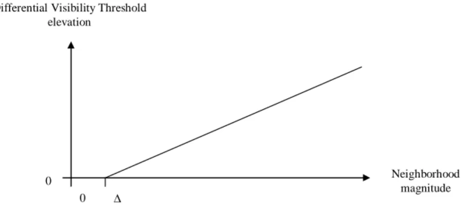
• The computation of the differential visibility threshold elevation : this re-produces the local variation of the differential visibility threshold due to the background content (masking effect).
Initially, luminance values are normalized by the mean luminance value to build a contrast image. This contrast image is then transformed according to Daly’s CSF in order to balance the spatial frequencies in a psychophysical way
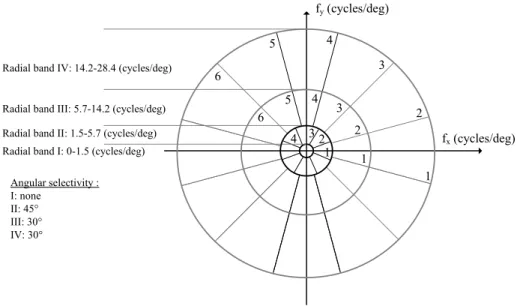
[31]. After the CSF has been applied, a perceptual subband decomposition is then applied. This decomposition is a psychophysical partitioning of the spatial frequency domain, both in radial spatial frequency and orientation.
To do that, the achromatic component image is decomposed in subband images by the use of 17 Cortex filters [32], as shown in figure 4. This decomposition has been designed in our lab in the past for CRT TV images coding through many visual tests [33]. For the sake of simplicity, although it has been shown that they are also decomposed into some perceptual subbands but quite fewer than for component A [34], chromatic components (Cr1 and Cr2) are not de-composed in subband images since they contain little structural information.
At last, Daly’s masking effect model is also employed to get data which are closer to perception.
The intra-channel and intra-component masking effect are computed. These computations consist of calculating, at each location (x, y) for each subband, the local DVT elevation which is due to the presence of a masking signal in the neighborhood. This is just a DVT elevation since the DVT has already been applied using the CSF. The shape of the function of elevation with respect to the masking signal magnitude is represented in figure 5.
fy(cycles/deg) 3 3 2 6 1 2 1 4 32 1 Angular selectivity : I: none II: 45° III: 30° IV: 30° fx(cycles/deg)
Radial band II: 1.5-5.7 (cycles/deg) Radial band I: 0-1.5 (cycles/deg)
4 5 6
4 5
Radial band III: 5.7-14.2 (cycles/deg) Radial band IV: 14.2-28.4 (cycles/deg)
Fig. 4. Psychophysical spatial frequency partitioning of the achromatic component A
Neighborhood magnitude Differential Visibility Threshold
elevation
0 ∆
0
Fig. 5. Differential visibility threshold elevation with respect to the masking signal magnitude
The local DVT elevation is given by the following relationship [31] : elevationρ,θ(x, y) = (1 + (k1∗ (k2∗ |Isbρ,θ(x, y)|)s)b)
1
b (2)
with :
• k1 = 0.0153
• k1 = 392.5
• Isbρ,θ(x, y) : amplitude at location (x, y) in the subband of indexes (ρ, θ) (ρ
represents the index of a radial subband and θ indicates the index of the directional subband),
• s, b : parameters depending on the considered radial frequency subband.
4.3 Selection of characteristic points and features extraction
Characteristic points determine locations where features will be extracted. Since these features are extracted in the subband images, the coordinates of a characteristic point are (x, y)ρ,θ.
Several approaches are possible to select these characteristic points : they can be selected arbitrarily or depending on the image content. The second ap-proach is more complicated than the first. Indeed it is difficult to determine interesting locations (for image quality assessment) in an image since this in-terest is determined partly at a semantic level. Moreover, the first approach presents an advantage in a RR context : arbitrary characteristic point’s coor-dinates don’t have to be transmitted (so it lowers the size of the RR).
For these reasons, the image quality criterion described in this paper selects characteristic points which are regularly distributed on concentric ellipses cen-tered at the image center, as shown in figure 6.
For each characteristic point, with spatial coordinates (x, y) being arbitrarily determined, the subband (ρ, θ) showing the greatest magnitude at this location is selected. If one considers that the signal in each subband (except the low radial frequency subband) can be seen as an image of waves of different orien-tations and different spatial frequencies as shown in figure 7 (right hand part), this selection corresponds to memorizing the most important wave magnitude at location (x, y). The number of ellipses and the number of characteristic points can vary. For the results shown in this paper, 16 characteristic points are selected on each ellipse. 22 concentric ellipses are used, leading to N = 352 characteristic points. With this constant number of characteristic points per ellipse, these points are more concentrated in the image center which generally gathers the parts of interest in images [35]. Even if the characteristic point selection is partially independent from the image content (independent for coordinates (x, y), dependent for subband number (ρ, θ)), features which are extracted from this point are fully dependent on image content.
Fig. 6. Characteristic points locations regularly located on concentric ellipses cen-tered at the center of the image
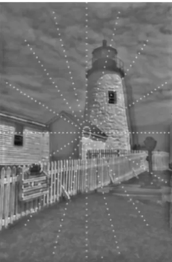
Fig. 7. Feature extraction in a subband on image “lighthouse1” from the LIVE scored images database: tested image (left), subband image of indexes ρ = III and θ= 1 (right) and example of an extracted segment (zoomed part)
The low radial frequency subband (0 to 1.5 cycles/degree) is not considered in this selection in order to have characteristic points belonging to structures of the image (a structure generates two main waves : a positive wave and a negative one). This mode of selecting characteristic points is illustrated in fig-ure 6 (in this figfig-ure, the background images are the sum of all the subbands used in the selection process (except the low radial frequency subband).
An approach was also tested in which the characteristic points were selected on locations which were fully dependent on image content. But this approach did not provide results as good as the ones obtained with the previously detailed selection method using predefined (x, y) coordinates. This can be explained by the fact that it is difficult to determine regions of real interest from a human point of view. Therefore, in order to limit the complexity of the quality assess-ment issue, the characteristic points have been selected using the concentric ellipses and so they regularly cover the image surface.
Perceptual features are extracted from each characteristic point Pi (i = 1..N)
and its neighborhood. The extracted features characterize the neighborhood of characteristic points in terms of oriented segments with contrast computed at different resolutions. Such features correspond to the type of information which is extracted in area V1 of the HVS since they indicate the orientation, length, width and magnitude of the contrast at the characteristic point.
The oriented segments are extracted by a stick growing algorithm as described in figure 7. Basically, a stick growing algorithm tries to build a segment, cen-tered in Pi, in all the possible directions and keeps the longest one. Each
segment point must be located on a value which is greater than a threshold expressed with respect to the value at the center of the segment (which is the characteristic point). A threshold value of 50% is used since it produces segments which are comparable to those one would manually extract to lo-cally represent the image content. Once the length Li and orientation Oi of
the segment have been determined, the stick growing algorithm is employed in the orthogonal direction in order to determine the segment width Wi. At last,
the amplitude Ami of the image subband is measured at characteristic point
Pi. The stick growing algorithm is faster than using more common methods
like filter banks for example since this algorithm is mainly composed of mem-ory address computations and threshold comparisons. A similar processing is used in [36]. Finally, for a characteristic point Pi, the extracted features are
described by the following parameters : orientation Oi, length Li, width Wi
and amplitude Ami.
The mean values of components A, Cr1 and Cr2 at characteristic point Pi
(called respectively features Ai, Cr1i and Cr2i) are also extracted. Each mean
value is computed over a neighborhood which corresponds to 0.2 visual degree of visual angle (this neighborhood corresponds in one dimension to 1/10th
of the foveal visual field [37]. This radius value was determined in order to measure a very local mean value.
So the reduced description of an image is composed of all the extracted features for each characteristic point Pi : Oi, Li, Wi, Ami, Ai, Cr1i and Cr2i. This
reduced description is generic since its features are not designed for predefined distortion types. However, the building of this reduced description requires to choose a type of display device and the normalized distance of viewing it. Therefore it targets the applications that correspond to these conditions.
5 Objective quality assessment
To assess the quality of a distorted image in a RR image quality criterion, the reduced description of the distorted image (RDDistorted) is compared to that of
its reference image (RR). Since the way by which the HVS compares features from the visual field and features from the visual memory is not precisely known yet, quite simple computations will be used in a logical order. Firstly local similarities will be measured, secondly these local similarity measures will be combined to produce a global similarity measure. This approach is close to the HVS behavior since the HVS precisely focusses on small regions of the visual field (the size of the foveal visual field is approximatively 2 degrees), so
one moves the eyes to focus to specific locations and fuses in an appropriate way these perceptions into a global representation.
At first, a “correspondence coefficient” C(FR,i, FD,i) is computed. This
corre-spondence coefficient indicates the similarity between feature FR,i (from RR)
and feature FD,i (from RDDistorted). Features FR,i and FD,i must be of the same
type : for example the correspondence coefficient is computed between two lengths (in this case F stands for L) or between two local mean values of component A (in that case F stands for A). They also have to be extracted from the same characteristic point Pi, which means from the same location
in the image plane (reference and distorted one respectively). Then, for each characteristic point Pi, several correspondence coefficients C(FR,i, FD,i) and
so several features types are combined to produce a local similarity measure LSi. At last, a global similarity measure S is calculated. S is defined as a
combination of local similarities LSi computed for each characteristic point
Pi (i = 1..N). S has to be well correlated with subjective quality scores. The
entire process is described in figure 8.
(Performance) Correlation
Used
RDref (= RR)
Reference image data
RDdist
Distorted image data
Correspondence coefficients computation Local similarity computation Global similarity computation
Similarity Measure
Subjective quality assessment tests with
human observers Mean Opinion Score (MOS) Display device gamma function
Perceptual colorspace Luminance dynamic normalization
CSF Subband decomposition
Masking effect model Features extraction Display device gamma function
Perceptual colorspace Luminance dynamic normalization
CSF Subband decomposition
Masking effect model Features extraction
Fig. 8. Full process of the objective quality criterion
combinations can be conceived. Several types of local similarity metrics were tested. Actually, 33 local similarity metrics have been tested and compared. These metrics differ by the number and types of features they used and by the way correspondence coefficients are combined (basically, either by an arith-metic averaging or by a geometric one). A study dedicated to comparing the different metrics can be found in [38]. Here, one of the most efficient similarity metrics is presented.
Typically, a correspondence coefficient C(FR,i, FD,i) between two features FR,i
(from RR) and FD,i(from RDDistorted) is directly a function of the absolute
dif-ference between the two features, normalized by the magnitude of the feature from the reference image. It is given by the following relationship:
C(FR,i, FD,i) = max(0, 1 −
FR,i− FD,i FR,i ) (3)
For features which are of orientation type (orientation of the extracted seg-ment), there would be no sense in normalizing the absolute difference ∆θ = |θR,i− θD,i| by the orientation of the segment from the reference image. So the
definition of the correspondence coefficient has been modified for this type of features. Since the biggest difference between two orientations is π/2, a func-tion of period π is used. The sense of orientafunc-tion is not taken into account: θ and θ + π give the same result. So the definition of the correspondence coeffi-cient between θR,i and θD,i is given by:
C(θR,i, θD,i) = 1 − 2∗∆θπ if ∆θ ≤ π2
C(θR,i, θD,i) = 2∗(∆θ− π 2)
π otherwise
A local similarity LSi combines the correspondence coefficients from different
features types. Local similarity at characteristic point Piis defined as the mean
value of correspondence coefficients taken from the set of selected features. The local similarity metric presented in this paper is the following function using the correspondence coefficients of all the 7 following features : Oi, Li, Wi, Ami,
A, Cr1 and Cr2 (as defined above).
LSi=
1
7[C(0R,i, 0D,i) + C(LR,i, LD,i) + C(WR,i, WD,i) + C(AmR,i, AmD,i) +C(AR,i, AD,i) + C(Cr1R,i, Cr1D,i) + C(Cr2R,i, Cr2D,i)] (4)
Here all the correspondence coefficients have the same weighting factor and it would be possible to use another combination and to apply some train-ing to determine these weighttrain-ing factors. This would probably improve the
performances of the quality measurement. Nevertheless, it would be hard to justify it from a biological point of view and it addresses high level of human perception. This could probably be studied deeply through psychophysics ex-periments and is already a subject of new research but this is out of the scope of this paper.
Finally, the global similarity S is defined in a very simple way as the mean value of local similarities LSi. S can viewed as an objective quality score
ranging from 0 to 1. S = 1 N N X i=1 LSi (5)
Correspondence coefficients as well as local similarities and global similarities range from 0 to 1.
If the way to compute the glocal similarity is quite simple, it is worth to note that the center of the image has more characteristic points than the border and so contributes more to the global similarity computation.
To produce an objective quality score Nobj with the same range as the sub-jective scores, the criterion presented in this paper uses a transformation of S. The choices concerning this transformation will be presented in the following section.
6 Performances
6.1 Introduction
Classicaly, the subjective quality score of a distorted image is the average of a set of indivual quality scores given by human observers during tests realized in normalized viewing conditions and according to a specific protocol. To measure the performances of an objective image quality criterion, the objective quality scores produced by this latter must be compared to subjective quality scores given by human observers. For this purpose, a database of scored images, which contains images and their subjective quality scores, has to be used. The mean value of the subjective quality scores for a given image is usually called the Mean Opinion Score (MOS). Many authors transform the value V produced by their criterion into an objective quality score using the following non-linear function whose parameters are optimized on the tested database :
Nobj = a
1 + exp(b ∗ (V − c)) (6)
In this paper, V corresponds to the global similarity S.
This transformation is described in the performance evaluation procedures employed by the Video Quality Experts Group (VQEG) Phase I FR-TV test [39]. The performances of the objective quality criterion presented here which is called “C4” (standing for “Criterion v4.0”) have been measured using this technique.
Once the objective quality scores have been computed, they are compared to the MOS (scores given by human observers). To perform this comparison, the Video Quality Expert Group (VQEG) has defined several metrics [39] which qualify the performances in terms of correlation (linear correlation coefficient), accuracy (standard deviation of the prediction error, standard deviation of the prediction error balanced by the confidence interval at 95% on the MOS), monotonicity (rank order correlation coefficient : RCC), consistency (outliers ratio) and agreement (Kappa coefficient).
6.2 Performances measurement methodology
The performances of an image quality criterion depends on the tested database. Several factors characterize such a database: image contents, image formats, type of distortions, display device, viewing conditions and subjective tests pro-tocol. In this paper, three different databases are used to perform an extended analysis of the performances. Indeed, since the performances of an image qual-ity criterion is dependent on the database used to test it, it is all the more important to use different databases. This matter of fact is also considered for video quality criteria in the scope of VQEG activities where models are tested according to different databases. Table 6.2 presents the databases that were tested to determine the performances of the image quality criterion proposed in this paper.
Database Image formats Type of Methodology Display Viewing
distortions device conditions
IVC 512x512 DCT coding, Double CRT ITU-R BT.500
DWT coding, Stimulus (distance
Locally Impairment and room
Adaptative Scale illumination)
Resolution (DSIS) coding (LAR),
Blurring
LIVE Various widths DCT Single CRT no restrictions
(from 480 to coding, Stimulus on viewing
768 pixels) and DWT Continuous distance and
various heights coding Quality normal
(from 438 to Scale indoor
720 pixels) (SSCQS)
Toyama 768x512 DCT Absolute LCD ITU-R BT.500
coding, Category adapted to
DWT Rating LCD (distance
coding (ACR) and room
illumination) Table 1
Tested databases and their characteristics to measure the image quality criterion performances
As shown in table 6.2, the image quality criterion has been tested with: • images of different sizes : fixed size (512x512 pixels) or various sizes (various
widths from 480 to 768 pixels and various heights from 438 to 720 pixels), • different distortions types : JPEG (DCT based), JPEG2000 (DWT based)
and LAR (neither DCT or DWT based, but based on a quadtree decompo-sition that defines a grid that allows to have locally adaptative resolution ),
• different display device types : CRT or LCD, • different protocols : DSIS, SSCQS or ACR,
For a purpose of comparison, UQI and SSIM criteria performances have also been computed on each database. UQI is an objective image quality criterion which is easy to calculate and which models any image distortion as a combi-nation of three factors: loss of correlation, luminance distortion, and contrast distortion [5]. SSIM is an improved version of UQI which uses structural dis-tortion as an estimate of perceived visual disdis-tortion [40].
6.2.1 Description of the IVC images database
The “IVC database of scored images” database contains images (and their cor-responding MOS) which have been distorted by 3 types of lossy compression techniques (JPEG, JPEG2000 or LAR : Locally Adaptative Resolution), or which have been blurred. The LAR coding [41] is based on the segmentation of the image into regions which are then quantized and coded individually. The IVC scored images database contains 50 JPEG images, 50 JPEG2000 images, 40 LAR images and 10 blurred images, leading to a set of 150 dis-torted images. The range of the distortions has been carefully selected in order that all the range 1-5 of visual quality can be achieved by each of these types of distortions process. The 10 reference images used to gener-ate this scored images database are well known in image processing literature : PEPPER, MANDRILL, LENA, ISABELLE, HOUSE, FRUITS, CLOWN, BOATS, BARBARA, PLANE. These images are presented in figure 9.
The DSIS (Double Stimulus Impairment Scale) protocol was employed and ITU recommendations concerning the viewing distance and room illumination were respected. The subjective scores result from subjective tests made in the IVC lab. During these tests, observers were asked to score the quality of the images which were presented under normalized conditions on a CRT Standard Definition TV monitor (background luminance of 10.5 cd/m2, viewing distance
of 6.H). The provided subjective quality scores come from an impairment scale ranging from 1 to 5 (1=“very annoying”, 2=“annoying”, 3=“slightly annoying”, 4=“perceptible but not annoying”, 5=“not perceptible”).
6.2.2 Description of the LIVE images database
To have more insight into assessing the performances of objective quality cri-terion C4, another database of scored images has also been tested: the LIVE database which contains JPEG and JPEG2000 coded images (with their MOS) and is freely available through the Internet [42]. In the LIVE database, quality scores range from 1 to 100. The reference images of the LIVE database are presented in figure 10.
Fig. 10. Reference images of the LIVE scored images database
Concerning the employed protocol, the notice provided with the database mentions :
”Observers were asked to provide their perception of quality on a continuous linear scale that was divided into five equal regions marked with adjectives Bad, Poor, Fair, Good and Excellent. The scale was then converted into 1-100
linearly. The testing was done in two sessions with about half of the images in each session. No viewing distance restrictions were imposed, display device configurations were identical and ambient illumination levels were normal in-door illumination. Subjects were asked to comfortably view the images and make their judgements. A short training preceded the session.”
Therefore the information provided with the LIVE database don’t enable to say that the protocol was one of those recommended by the ITU. Neverthe-less the procedure seems to have lots of similarities with the SSCQS (Single Stimulus Continuous Quality Scale) protocol.
6.2.3 Description of the Toyama images database
For this database, Toyama’s university has defined a range of distortions that uniformly covers the quality scale. The reference images come from the LIVE database. The reference images of the Toyama database are presented in figure 11.
Fig. 11. Reference images of the Toyama scored images database
Using Toyama’s images, the IVC research team realized subjective quality assessment tests with the ACR (Absolute Category Rating) protocol. This protocol consists in presenting the images one at a time. Each image was pre-sented during 10 seconds then observers judged them using a 5 grade quality scale containing the following categories: excellent, good, fair, poor, bad. The ACR enables to collect many judgements rapidly but since it doesn’t allow the observers to compare the judged images with their reference images, the votes precision may be lower with this protocol compared to other protocols with reference presentation, like DSIS. So, more observers are generally required in order to get a good precision measured by computing the confidence interval
on the Mean Opinion Scores (MOS). Concerning the viewing conditions dur-ing these tests, users watched the images at a distance of 4 times the height of the image displayed on a LCD TV monitor.
6.3 Performances on the IVC images database
The performances of criterion “C4” are presented in table 6.3 according to the VQEG performances metrics. For the purpose of comparison, MSE and PSNR criteria performances are also given.
C4 UQI SSIM MSE PSNR
Linear Correlation Coefficient (CC) 0.913 0.809 0.779 0.543 0.633 Rank order Correlation Coefficient (RCC) 0.909 0.804 0.791 0.632 0.632 Error standard deviation (σǫ) 0.495 0.713 0.762 1.020 0.940 Balanced error standard deviation (σWǫ ) 0.470 2.891 2.504 5.13 5.11 Kappa coefficient (Kappa) 0.521 0.370 0.359 0.147 0.218
Outliers ratio (OR) 5.33% 12% 17.33% 32.67% 26.67% Table 2
Performances of C4 and others criteria on 150 images (JPEG, JPEG2000, LAR, blurred) from the IVC database of scored images (DSIS)
These results show that criterion C4 provides quality scores that are well correlated with human judgments (CC and RCC are greater than 0.9). The standard deviation of the prediction error is quite acceptable (σǫ = 0.495 on
a quality scale ranging from 1 to 5). The standard deviation of the error bal-anced by the confidence interval at 95% on the MOS is lower than 0.5. This means that, on average, the objective quality score produced by the criterion C4 for an image is closer to the MOS than the subjective quality score given by an observer chosen randomly. The Kappa coefficient is greater than 0.4 which is the threshold defined by the VQEG to determine wether an image quality criterion is efficient or not. At last, the outliers ratio is quite low (OR = 5.33%) so few images are badly scored by C4. Compared to criterion C4, UQI and SSIM have significantly lower performances (CC and CC are both
around 0.8 only). As expected, MSE and PSNR criteria show the worst per-formances.
On the IVC database, optimal parameters values in the final construction of the objective quality score (for criterion C4) are a = 5.667, b = 15.971 and c = 0.827.
6.4 Performances on the LIVE scored images database
Performances measurement results obtained on the LIVE scored images database are presented in table 3 for JPEG images and in table 4 for JPEG2000 im-ages, once again along with the performances of UQI, SSIM, MSE and PSNR criteria, for comparison.
C4 UQI SSIM MSE PSNR
Linear Correlation Coefficient (CC) 0.972 0.907 0.958 0.750 0.858 Rank order Correlation Coefficient (RCC) 0.953 0.893 0.943 0.884 0.843 Error standard deviation (σǫ) 5.013 9.036 6.190 10.895 7.858 Balanced error standard deviation (σW ǫ ) 0.421 0.753 0.572 1.018 0.654
Kappa coefficient (Kappa) 0.834 0.662 0.781 0.454 0.513 Outliers ratio (OR) 1.96% 15.69% 10.29% 29.41% 10.86% Table 3
Performances of C4 and other criteria on 204 JPEG images from the LIVE database of scored images (SSCQS)
Here again, results show that the objective quality criterion C4 maintains good performances with different images databases (IVC database and JPEG images from the LIVE database) and so for a variety of contents with various distortion types. These results also show that this criterion is efficient for a range of distortions but performs better when it is limited to a given distortion process. This can be explained by the fact that different distortion processes have different impacts on quality. Therefore, for a fixed quality level, a given process can introduce more distortions than another one. Thus, the variations
of similarity measures are different from one distortion process to another. Hence, the correlation between global similarity measures and MOS is greater when the tested images are limited to only one distortion type. In addition, the fitting function parameters a, b and c enable a better correspondence between MOS and Nobj, leading to a higher correlation coefficient (CC = 0.972). On the JPEG images from the LIVE database, optimized parameter values of the fitting function for criterion C4 are a = 117.425, b = 6.125 and c = 0.857 (note that the quality scale now ranges from 1 to 100).
C4 UQI SSIM MSE PSNR
Linear Correlation Coefficient (CC) 0.957 0.881 0.942 0.754 0.880 Rank order Correlation Coefficient (RCC) 0.951 0.876 0.941 0.902 0.879 Error standard deviation (σǫ) 6.010 9.827 7.016 10.725 7.339 Balanced error standard deviation (σW ǫ ) 0.480 0.751 0.543 0.822 0.491
Kappa coefficient (Kappa) 0.883 0.370 0.359 0.147 0.218 Outliers ratio (OR) 4.55% 16.16% 6.06% 27.78% 7.10% Table 4
Performances of C4 and others criteria on 198 JPEG2000 images from the LIVE database of scored images (SSCQS)
Table 4 provided the results got with the JPEG2000 images of the LIVE database. They are very similar to those obtained with the JPEG images of the LIVE database. The quality scores produced by criterion C4 are highly correlated to the subjective ones (CC and CCR are greater than 0.95) and the standard deviation of the prediction error is low and quite acceptable (6.01 on a 100-grade scale). The balanced standard deviation is still lower than 0.5. The Kappa coefficient of criterion C4 is much higher than the threshold value of 0.4 defined by the VQEG. More, the Kappa coefficient is lower than 0.4 for all other criteria, indicating that C4 is the only efficient criterion among the tested ones. At last, the outliers ratio is low for criterion C4 (4.55%) showing that few images are badly scored. All these results confirm that criterion C4 performs very well when it is limited to a single distortion process.
From a different point of view, it can also be noticed that PSNR provides a rather good correlation with subjective quality scores on the LIVE database
(CC=0.858 with JPEG images and CC=0.880 with JPEG2000 images). This can be partially explained by the fact that some of the images in this database are heavily distorted, producing often very low quality scores. These images are more easily scored by PSNR which works better with heavy distortions than with subtle ones.
On the JPEG2000 images from the LIVE database, the optimal parameters values for criterion C4 are a = 103.720, b = 8.185 and c = 0.828.
6.5 Performances on the Toyama scored images database
For the Toyama scored images database, the performances of criterion C4 are presented in table 6.5 for JPEG2000 images and in table 6.5 for JPEG images. In order to briefly demonstrate the performances of criterion C4 on these images which were displayed on a LCD device, only the linear and rank correlation coefficients are given.
C4 UQI SSIM Linear Correlation Coefficient (CC) 0.934 0.785 0.916 Rank order Correlation Coefficient (RCC) 0.945 0.780 0.915 Table 5
Performances of C4 and others criteria on 98 JPEG2000 images from the Toyama database of scored images (ACR)
C4 UQI SSIM Linear Correlation Coefficient (CC) 0.887 0.781 0.660 Rank order Correlation Coefficient (RCC) 0.887 0.773 0.660 Table 6
Performances of C4 and others criteria on 84 JPEG images from the Toyama database of scored images (ACR)
These last results indicate that criterion C4 also gives good results to measure the visual quality of images which are displayed on a LCD device. Perfor-mances are better for JPEG2000 images than for JPEG images but, for both
cases, criterion C4 provides more accurate quality scores than criteria UQI and SSIM criteria.
6.6 Conclusions on the three tested databases
First, it can be noticed that the image quality criterion proposed here pro-vides more accurate quality scores than state-of-the-art UQI and SSIM criteria (which are full reference quality criteria) on the three tested databases. This is not obvious since the proposed image quality criterion is a RR criterion whereas UQI and SSIM are FR criteria. These superior performances can be explained by the fact that the proposed criterion includes a model of the dis-play device (non linear transformation) and an elaborate model of the human vision (perceptual colorimetric colorspace, CSF, masking effect).
In addition, the proposed image quality criterion gives a good prediction of human judgements for images of different sizes, different distortions types, different display device types, different protocols and different viewing con-ditions. Therefore this objective quality criterion can be considered as being robust.
7 Conclusion
In this paper, the different categories of already existing quality criteria have been presented, especially the reduced reference criteria. A new quality crite-rion called C4 has also been presented for color images. This critecrite-rion imple-ments an operating and organisational model of the HVS, including some of the most important stages of vision (perceptual color space, CSF, psychophysi-cal subband decomposition, masking effect modeling). The novelty of this work is that criterion C4 extracts structural information from the representation of images in a perceptual space. Extracted features are stored in a reduced de-scription which is generic as it is not designed for specific types of distortions. Performances were tested on three different databases of scored images (con-taining images and their MOS) using VQEG performances measurement tech-niques. Results show that criterion C4 provides quality scores which are highly correlated with MOS collected from human observers. Good correlation coef-ficients were measured on these images databases : CC=0.913 on 150 images from the IVC database, CC=0.972 on 204 JPEG images of the LIVE database, CC=0.957 on 198 JPEG2000 images of the LIVE database, CC=0.934 on 98 JPEG images of the Toyama database, CC=0.887 on 84 JPEG2000 images of the Toyama database. The results indicate that criterion C4 provides much better performances than classical RMSE or PSNR methods and that it
com-petes favorably with state-of-the-art criteria like UQI and SSIM which are full reference quality criteria. Quality assessment can be generic but performs bet-ter when tested images are limited to a given type of coding scheme. No image has been used in the design of the presented criterion which can be applied to any type of images. At last, in order to facilitate the use of the presented quality criterion, software applications which implement it are freely available on the Internet at URL http://membres.lycos.fr/dcapplications/index.php.
References
[1] R. Lancini, F. Mapelli, and S. Saviotti, “Video quality analysis using a watermarking technique,” in Proceedings of ICIP (IEEE International Conference on Image Processing), Singapore, 24-27 October 2004.
[2] F. X. J. Lukas and Z. L. Budrikis, “Picture quality prediction based on a visual model,” in IEEE Transactions on Communications, Vol. 30, Issue 7, pp. 1679– 1692, 1982.
[3] Z. Wang, H. R. Sheikh, and A. C. Bovik, “No-reference perceptual quality assessment of jpeg compressed images,” in Proceedings of ICIP (IEEE International Conference on Image Processing), 2002.
[4] C. Zetzsche and G. Hauske, “Multiple channel model for the prediction of subjective image quality,” in Human Vision, Visual Processing, and Digital Display, SPIE Vol. 1077, pp. 209–216, 1989.
[5] Z. Wang and A. C. Bovik, “Universal quality index,” in IEEE Signal Processing Letters, Volume 9, Issue 3, pp. 81–84, March 2002.
[6] S. D. Voran and S. Wolf, “The development and evaluation of an objective video quality assessment system that emulates human viewing panels,” in Proceedings of International Broadcasting Convention, Amsterdam, The Netherlands, 1992. [7] A. A. Webster, C. T. Jones, M. H. Pinson, S. D. Voran, and S. Wolf, “An objective video quality assessment system based on human perception,” in SPIE Human Vision, Visual Processing, and Digital Display IV, San Jose, CA, pp. 15–26, February 1993.
[8] S. Wolf, A. Webster, M. Pinson, and G. Cermak, “Objective and subjective measures of mpeg video quality,” tech. rep., ANSI contribution number T1A1.5/96-121, 1996.
[9] Z. Wang and E. P. Simoncelli, “Reduced-reference image quality assessment using a wavelet-domain natural image statistic model,” in Proceedings of SPIE Human Vision and Electronic Imaging X, Vol. 5666, San Jose, CA, pp. 149– 159, 2005.
[10] T. M. Kusuma and H.-J. Zepernick, “On perceptual objective quality metrics for in-service picture quality monitoring,” in 3rd ATcrc Telecommunications and Networking Conference and Workshop, Melbourne, Australia, Dec. 2003. [11] Z. Wang, A. C. Bovik, and B. L. Evans, “Blind measurement of blocking
artifacts in images,” in Proceedings of IEEE International Conference on Image Processing, Volume 3, pp. 981–984, 2000.
[12] P. Marziliano, F. Dufaux, S. Winkler, and T. Ebrahimi, “A no-reference perceptual blur metric,” in Proceedings of IEEE International Conference on Image Processing, Vol. 3, Rochester, NY, USA, pp. 57–60, 2002.
[13] S. Saha and R. Vemuri, “An analysis on the effect of image activity on lossy coding performance,” in Proceedings of IEEE International Symposium on Circuits and Systems, Volume 3, Geneva, Switzerland, pp. 295–298, 2000. [14] M. Carnec, P. Patrick Le Callet, and D. Barba, “A human visual system
model for image quality assessment,” in Proceedings of IMAGE 2003, Sarawak, Malaysia, 21-22 april 2003.
[15] M. Carnec, P. L. Callet, and D. Barba, “A new method for perceptual quality assessment of compressed images with reduced reference,” in Proceedings of Picture Coding Symposium, Saint Malo, France, pp. 343–348, April 23-25, 2003. [16] A. C. Huk and D. J. Heeger, “Task-related modulation of visual cortex,” in
Journal of Neurophysiology, Vol. 83, pp. 3525–3536, 2000.
[17] D. H. Hubel and T. N. Wiesel, “Receptive fields and functional architecture of monkey striate cortex,” in Journal of Physiology, Volume 195, Issue 1, pp. 215– 243, 1968.
[18] F. Crick and C. Koch, “Consciousness and neuroscience,” in Cerebral Cortex, Vol. 8, pp. 97–107, 1998.
[19] S. M. Zeki, “Functional organization of a visual area in the posterior bank of the superior temporal sulcus of the rhesus monkey,” in Journal of Physiology, Vol. 236, Issue 3, pp. 549–573, 1974.
[20] T. Kuyel, W. Geisler, and J. Ghosh, “Retinally reconstructed images (RRIs): Digital images having a resolution matching with the human eye,” in Proceedings of SPIE Human Vision and Electronic Imaging III, Vol. 3299, San Jose, CA, pp. 603–614, 1998.
[21] H. C. Nothduft and C. Y. Li, “Texture discrimination: Representation of orientation and luminance differences in cells of the cat striate cortex,” in Vision Research, Vol. 25, Issue 1, pp. 99–113, 1985.
[22] D. H. Hubel and T. N. Wiesel, “Receptive fields of single neurones in cat’s striate cortex,” in Journal of Physiology, Vol. 148, Issue 3, pp. 574–591, 1959. [23] D. H. Hubel and T. N. Wiesel, “Receptive fields, binocular interaction and functional architecture in the cat’s visual cortex,” in Journal of Physiology, Vol. 160, Issue 1, pp. 106–154.2, 1962.
[24] W. Bechtel and R. N. McCauley, “Heuristic identity theory (or back to the future): The mind-body Problem Against the background of research strategies in cognitive neuroscience,” in Proceedings of the 21st Annual Meeting of the Cognitive Science Society, Vancouver, Canada, 1999.
[25] D. H. Hubel and T. N. Wiesel, “Receptive fields and functional architecture in two non-striate visual areas (18 and 19) of the cat,” in Journal of Physiology, Vol. 28, pp. 229–289, 1965.
[26] R. Desimone, S. J. Schein, J. Moran, and L. G. Ungerleider, “Contour, color and shape analysis beyond the striate cortex,” in Vision Research, Vol. 25, Issue 3, pp. 441–452, 1985.
[27] D. A. Pollen, “On the neural correlates of visual perception,” in Cerebral Cortex, Vol. 9, Issue 1, pp. 4–19, January 1999.
[28] W. H. Merigan, T. A. Nealey, and H. R. Maunsell, “V4 lesions in macaques affect both single and multiple-viewpoint shape discriminations,” in Visual Neuroscience, Vol. 15, pp. 359–367, 1998.
[29] P. Schiller, “The effects of v4 and middle temporal (mt) area lesions on visual performances in the rhesus monkey,” in Visual Neuroscience, Vol. 10, Issue 4, pp. 717–746, 1993.
[30] J. Krauskopf, D. R. Williams, and D. W. Heeley, “Cardinal directions of color space,” in Vision Research, Volume 22, Issue 9, pp. 1123–1131, 1982.
[31] S. Daly, The Visible Differences Predictor: An Algorithm for the Assessment of Image Fidelity, pp. 179–206. MIT Press, 1993.
[32] A. B. Watson, “The cortex transform : Rapid computation of simulated neural images,” in Computer vision, graphics and image processing, Volume 39, Issue 3, pp. 311–327, 1987.
[33] H. Senane, A. Saadane, and D. Barba, “Image coding in the context of a psychovisual image representation with vector quantization,” in Proceedings of IEEE International Conference on Image Processing, Washington, pp. 97–100, October 1995.
[34] P. Le Callet and D. Barba, “Robust approach for color image quality assessment,” in Proceedings of SPIE Visual Communications and Image Processing, Vol. 5150, Lugano, Switzerland, pp. 1573–1581, 2003.
[35] O. L. Meur, P. L. Callet, D. Barba, and D. Thoreau, “A coherent computational approach to model bottom-up visual attention,” in IEEE Transactions on Pattern Analysis and Machine Intelligence, Volume 28, Issue 5, pp. 802–817, 2006.
[36] G. C. Hunt and R. C. Nelson, “Lineal feature extraction by parallel stick growing,” in Proceedings of the Third International Workshop on Parallel Algorithms for Irregularly Structured Problems, Santa Barbara CA, pp. 171– 182, 1996.
[37] A. Murata and T. Miyoshi, “Trade-off relationship between width and depth of visualinformation processing in measurement of functional visual field,” in Proceedings of IEEE International Conference on Systems, Man, and Cybernetics, Volume 2, Nashville, Tennessee, USA, pp. 1271–1276, 2000. [38] M. Carnec, P. L. Callet, and D. Barba, “Visual features for image quality
assessment with reduced reference,” in Proceedings of IEEE International Conference on Image Processing, Volume 1, Genoa, Italy, pp. 421–424, 11-14 september 2005.
[39] A. M. Rohaly, P. Corriveau, J. Libert, A. Webster, V. Baroncini, J. Beerends, J. L. Blin, L. Contin, T. Hamade, D. Harrison, A. Hekstra, J. Lubin, Y. Nishida, R. Nishihara, J. Pearson, A. F. Pessoa, N. Pickford, A. Schertz, M. Visca, A. Watson, and S. Winkler, “Video quality experts group: Current results and future directions,” in Proceedings of SPIE Visual Communications and Image Processing, Vol. 4067, Perth, Australia, 3, pp. 742–753, 2000.
[40] Z. Wang, A. C. Bovik, H. R. Sheikh, and E. Simoncelli, “Image quality assessment: From error measurement to structural similarity,” in IEEE Trans. Image Processing 13, Jan. 2004, 2004.
[41] O. D´eforges and J. Ronsin, “Locally adaptative method for progressive still image coding,” in IEEE International Symposium on Signal Processing and its Applications, Vol. 2, Brisbane, Australia, pp. 825–829, 1999.
[42] H. R. Sheikh, Z. Wang, L. Cormack, and A. C. Bovik, “Live image quality assessment database.” http://live.ece.utexas.edu/research/quality.
Mathieu CARNEC was born in Plœmeur, France, on August 13, 1976. He received the Diplˆome d’Ing´enieur in electronics and computer en-gineering from ´Ecole Nationale d’Ing´enieurs de Brest (ENIB), France. In July 2004 he obtained a PhD in image processing from ´Ecole Poly-technique de l’Universit´e de Nantes, France. His research works focus on human visual system modeling and image and video quality assessment, especially for networks.
In 2004-2005, he taught computer science at Universit´e Paris 13 and belonged to the L2TI (Laboratoire de Traitement et de Transport de l’Information). Since 2005, he has been a reasearch engineer for a euro-pean project called HD4U which aims to deploy HDTV in Europe.
Patrick LE CALLET holds a PhD in image processing from the Uni-versity of Nantes. Engineer in electronics and computer science, he was also a student of the ´Ecole Normale Superieure de Cachan. In 1996, he received his agregation degree in electronics.
He is currently an Associate Professor at the university of Nantes, en-gaged in research dealing with the application of human vision modeling in image processing. His current centers of interest are image quality assessment, watermarking technique and saliency map exploitation in image coding techniques.
Dominique BARBA was born in France in 1944. He received a PhD in Telecommunications in 1972 and the degree of Doctorat es Sciences Math´ematiques (with honors) in Computer Science in 1981 in the field of digital image processing. He was an Associate Professor at INSA in RENNES from 1973 and, in 1985, he became a Professor at ´Ecole Poly-technique de l’Universit´e de Nantes where he launched a new research laboratory. His research interests include Pattern Recognition and Image Analysis, Image and Video description and compression Human visual system modeling with application to the design of objective image and video quality criteria. He is the author or co-author of more than 300 pa-pers in scientific journals or international and national conferences and is member of many science and technical societies (IEEE, SPIE, SEE, etc.).
List of Figures
1 Block diagram of a RR image quality criterion 4
2 Human Visual System model 6
3 Different stages used to build the reduced description of an
image (and the corresponding biological parts in the HVS) 9 4 Psychophysical spatial frequency partitioning of the achromatic
component A 11
5 Differential visibility threshold elevation with respect to the
masking signal magnitude 12
6 Characteristic points locations regularly located on concentric
ellipses centered at the center of the image 13
7 Feature extraction in a subband on image “lighthouse1” from the LIVE scored images database: tested image (left), subband image of indexes ρ = III and θ = 1 (right) and example of an
extracted segment (zoomed part) 14
8 Full process of the objective quality criterion 16
9 Reference images of the IVC scored images database 21
10 Reference images of the LIVE scored images database 22 11 Reference images of the Toyama scored images database 23
List of Tables
1 Tested databases and their characteristics to measure the
image quality criterion performances 20
2 Performances of C4 and others criteria on 150 images (JPEG, JPEG2000, LAR, blurred) from the IVC database of scored
images (DSIS) 24
3 Performances of C4 and other criteria on 204 JPEG images
4 Performances of C4 and others criteria on 198 JPEG2000
images from the LIVE database of scored images (SSCQS) 26 5 Performances of C4 and others criteria on 98 JPEG2000
images from the Toyama database of scored images (ACR) 27 6 Performances of C4 and others criteria on 84 JPEG images