Fast Computation of Sliding Discrete Tchebichef Moments and Its Application in Duplicated Regions Detection

(1)

HAL Id: hal-01217003

https://hal-univ-rennes1.archives-ouvertes.fr/hal-01217003

Submitted on 30 Oct 2015

HAL is a multi-disciplinary open access

archive for the deposit and dissemination of

sci-entific research documents, whether they are

pub-lished or not. The documents may come from

teaching and research institutions in France or

abroad, or from public or private research centers.

L’archive ouverte pluridisciplinaire HAL, est

destinée au dépôt et à la diffusion de documents

scientifiques de niveau recherche, publiés ou non,

émanant des établissements d’enseignement et de

recherche français ou étrangers, des laboratoires

publics ou privés.

Fast Computation of Sliding Discrete Tchebichef

Moments and Its Application in Duplicated Regions

Detection

Beijing Chen, Gouenou Coatrieux, Jiasong Wu, Zhifang Dong, Jean Louis

Coatrieux, Huazhong Shu

To cite this version:

Beijing Chen, Gouenou Coatrieux, Jiasong Wu, Zhifang Dong, Jean Louis Coatrieux, et al.. Fast

Computation of Sliding Discrete Tchebichef Moments and Its Application in Duplicated Regions

De-tection. IEEE Transactions on Signal Processing, Institute of Electrical and Electronics Engineers,

2015, 63 (20), pp.5424 - 5436. �10.1109/TSP.2015.2451107�. �hal-01217003�

(2)

Abstract— Computational load remains a major concern when processing signals by means of sliding transforms. In

this paper, we present an efficient algorithm for the fast computation of one-dimensional and two-dimensional sliding discrete Tchebichef moments. To do so, we first establish the relationships that exist between the Tchebichef moments of two neighboring windows taking advantage of Tchebichef polynomials’ properties. We then propose an original way to fast compute the moments of one window by utilizing the moment values of its previous window. We further theoretically establish the complexity of our fast algorithm and illustrate its interest within the framework of digital forensics and more precisely the detection of duplicated regions in an audio signal or an image. Our algorithm is used to extract local features of such a signal tampering. Experimental results show that its complexity is independent of the window size, validating the theory. They also exhibit that our algorithm is suitable to digital forensics and beyond to any applications based on sliding Tchebichef moments.

Index Terms: Tchebichef moments, sliding transform, fast computation, duplicated signal detection I. INTRODUCTION

Tchebichef moments or transforms were first introduced by Mukundan et al. [1]. Since the Tchebichef polynomials are orthogonal in the discrete domain of coordinate space, their implementation does not involve any numerical approximation. This property makes them superior to the conventional continuous orthogonal moments such as Legendre moments and Zernike moments [2-5]. Thus, Tchebichef moments have been extensively used in pattern recognition [5], texture classification [6], medical image reconstruction [7] and forensics [8]. Among these applications, local features play an important role and allow avoiding a whole segmentation of objects [9]. Local moments have been shown of interest for the detection of key features [10-13]. However, one of the main drawbacks in their use as local features is their computational load inducing the needs for fast computation. In this paper, we investigate the local discrete orthogonal Tchebichef moment properties when used over sliding windows and we propose a fast computation algorithm of sliding discrete Tchebichef moments (SDTMs).

Basically, the sliding orthogonal transform of a signal means that the transform is computed on a fixed-size window of the signal, which is continuously updated with new samples while discarding the older ones [14]. Let f(x) be the original signal with length L, and assume that the window at time instant p contains N values f(p), f(p+1), …, f(p+N-1), 0 ! p, p+N-1 < L, then, the sliding orthogonal transform is defined by [15,16]

1 0 ( )

!

( , ), 0,1,..., 1 " = =

#

N + = " p s m m Y f p m w m s s N , (1)

This work was supported by the National Basic Research Program of China under Grant 2011CB707904, the NSFC under Grants 61271312, 61103141, 61232016, 61173141, and 11301074, the Natural Science Foundation of the Jiangsu Higher Education Institutions of China under Grant 13KJB520015, a Project Funded by the Priority Academic Program Development of Jiangsu Higher Education Institutions, Open Fund of Jiangsu Engineering Center of Network Monitoring (KJR1404), Jiangsu Province under Grants DZXX-031, and BY2014127-11, and the Qing Lan Project.

Beijing Chen is with Jiangsu Engineering Center of Network Monitoring, School of Computer & Software, Nanjing University of Information Science & Technology, and also with Collaborative Innovation Center of Atmospheric Environment and Equipment Technology, Nanjing University of Information Science & Technology, 210044 Nanjing, China. Beijing Chen is also with the Institut Mines-Telecom, Telecom Bretagne, INSERM UMR1101 LaTIM, 29238 Brest, France (e-mail: nbutimage@126.com).

Gouenou Coatrieux is with the Institut Mines-Telecom, Telecom Bretagne, INSERM UMR1101 LaTIM, 29238 Brest, France (e-mail: gouenou.coatrieux@telecom-bretagne.eu). Jiasong Wu and Jean Louis Coatrieux are with the Laboratory of Image Science and Technology, School of Computer Science and Engineering, Southeast University, 210096 Nanjing, China, and also with the INSERM U1099, 35000 Rennes, France, with Laboratoire Traitement du Signal et de l’Image, Université de Rennes I, 35000 Rennes, France, and also with Centre de Recherche en Information Biomédicale Sino-Français (CRIBs), 35000 Rennes, France (e-mail: jswu@seu.edu.cn, jean-louis.coatrieux@univ-rennes1.fr).

Zhifang Dong is with School of Electronic Science & Engineering, Southeast University, 210096 Nanjing, China (e-mail: dongzhifang@seu.edu.cn).

Huazhong Shu is with the Laboratory of Image Science and Technology, School of Computer Science and Engineering, Southeast University, and also with Centre de Recherche en Information Biomédicale Sino-Français (CRIBs), 210096 Nanjing, China (e-mail: shu.list@seu.edu.cn).

Fast computation of sliding discrete Tchebichef moments and its

application in duplicated regions detection

Beijing Chen, Gouenou Coatrieux, Senior Member, IEEE, Jiasong Wu, Member, IEEE, Zhifang Dong, Jean Louis Coatrieux, Fellow, IEEE, and Huazhong Shu, Senior Member, IEEE

(3)

where wm is a window function, and

{ ( , )}

!

m s

is an orthogonal basis set. Ysprepresents the orthogonal transform of the

windowed signal around time p.

In the past decades, many works have been reported in the literature for the fast computation of sliding transforms. They can be classified into two categories: 1) the structures of radix-2 and radix-4 fast algorithms such as sliding FFT [17] , Hopping DFT [18], sliding Walsh Hadamard transform [19], sliding Haar transform [20], sliding conjugate symmetric sequency-ordered complex Hadamard transform [21]; 2) the first- and second- order shift properties of sliding transforms including sliding DFT [22, 23], sliding DCT [15], sliding DHT [16], sliding discrete fractional Fourier transform [24], sliding Walsh Hadamard transform [25], sliding Haar transform [26], modulated sliding discrete Fourier transform [27], and sliding geometric moment (SGM) [28].

In this paper, we suggest to utilize the first-order shift properties of SDTMs for their fast computation. The rest of this paper is organized as follows: Section II defines the one-dimensional and two-dimensional SDTMs. Some properties of orthogonal Tchebichef polynomials are reviewed. The proposed fast algorithm to compute SDTM and its computational complexity analysis are presented in Section III. Performance test and applications are reported in Section IV in the framework of digital forensics looking at the detection of duplicated signal segments or image regions. Section V concludes the paper.

II. PRELIMINARIES

A. Sliding discrete Tchebichef moment

According to the definition of the sliding orthogonal transform in (1), let us first introduce the 1-D SDTM for the orthogonal Tchebichef polynomials set. For a signal f(x) of length L, x = 0, 1, …, L–1, assume that the window of f(x) at time instant p contains N values f(p), f(p+1), …, f(p+N–1), 0 ! p, p+N–1 < L, then the nth order 1-D SDTM is defined as

1 0 ( ) ( ) N p n n x T ! f p x t x = =

"

+ , n = 0,1,…,N–1, (2)

where tn(x) is the nth order orthonormal Tchebichef polynomial defined by

2 0 (1 ) ( ) ( ) (1 ) ( ) , ( !) (1 ) ( , ) n n l l l n l l N n x n t x l N n N

!

= " " " + = "

#

n, x = 0,1,…,N–1. (3)

Here (a)l is the Pochhammer symbol

( )

a

l

=

a a

( 1)(

+

a

+

2) (

!

a l

+ !

1)

, l ! 1, and (a)0 = 1, (4)

and the squared-norm !(n, N) is given by

( )! ( , ) (2 1)( 1)! N n n N n N n

!

= + + " " . (5)

For an N"N block [p, p+N–1] " [q, q+N–1] of an image f(x, y) at position (p, q), the (n+m)th order 2-D SDTM is defined as

1 1 , , 0 0

(

,

) ( ) ( )

N N p q n m n m x y

T

! !

f p x q y t x t y

= =

=

""

+

, n, m = 0,1,…,N–1. (6)

B. Some properties of orthonormal Tchebichef polynomials [3]

In [3], Shu et al. established the following relationship between tn(x) at position x and tn(x+a) at position x+a,

0 0 ( ) n n l ( , )( ) ( ) n r r l l r t x a ! g n l a t x = = + =

""

! , (7) where (2 1)( 1 )! ( , ) ( 1) !( )!( 1 )! ( , ) ( 1) , !( 1 )! ( , ) ( )!( )!( 1)!( )!( 1 )! ! ! " = + " " " + + " " " = " " "

#

+ " " + + " " " s n r n r s l l N l l N s n r s N s r g n l r N n n N r s n r s s l s l N s 0 # l # n. (8) When a = 1 in (7), we have

(4)

1 ₁ 0 ( 1) ( ) n ( , ) ( ) n n l l t x t x ! g n l t x = + = !

"

, (9) where g1(n, l) is defined by (8).

III. FAST COMPUTATION OF SLIDING DISCRETE TCHEBICHEF MOMENTS AND ITS COMPUTATIONAL COMPLEXITY

In this section, we propose an efficient algorithm for the fast computation of 1-D SDTMs defined by (2) and 2-D SDTMs by (6). We also analyze its computational complexity.

A. Fast algorithm of 1-D sliding discrete Tchebichef moments

According to 1-D SDTM defined in (2), the 1-D SDTM at time instant p+1 is given by

1 1 0 ( 1 ) ( ) N p n n x T + ! f p x t x = =

"

+ + , n = 0, 1, …, N–1. (10)

Equation (10) can be rewritten as

1 2 0 ( 1) ( ) N ( 1 ) ( ) p n n n x T + t N f p N ! f p x t x = = ! + +

"

+ + . (11)

Similarly, (2) can also be rewritten as

2 0 (0) ( ) N ( 1 ) ( 1) p n n n x T t f p ! f p x t x = = +

"

+ + + . (12)

Using (9), (11) and the symmetry property

(

1 ) ( 1) ( ),

n

n n

t N

! ! = !

x

t x

(13) as well as making the notation g1(n, n) = –1, the second term in (12) becomes

2 0 2 1 2 1 0 0 0 1 1 1 1 0 1 1 0 ( 1 ) ( 1) ( 1 ) ( ) ( , ) ( 1 ) ( ) ( 1) ( ) ( , ) ( 1) ( ) ( , ) ( 1) (0) ( ) . N n x N n N n l x l x n p p n n l l l n p l l l l f p x t x f p x t x g n l f p x t x T t N f p N g n l T t N f p N g n l T t f p N ! = ! ! ! = = = ! + + = + = + + + = + + ! + + " # = ! ! + ! _$ ! ! + _% " # = ! _$ ! ! + _%

&

(14)

By introducing (14) into (12), for all the moments up to order M, M < N, (12) can be expressed in a matrix form as 1 0 0 1 1 1 1 ( ) ( ) ( ) ( ) . ( 1) ( ) ( ) + + + ! + " ! " # $ # $ ! " %' ( & % & ' ₎ ₊ ( % & %' ( & % &_{= )} ₎ ' ( ₊ % & %' ( & % & ' ( % & %' ( & % & _' ₍ ' ₎ ₊ ( % & % & % * +& , -, - ,* + -! ! ! ! p p p p M M M M p p M M f p N f p T T f p N f p T T A B B f p N f p T T (15) where 1 1 1 1 1 1 1 1 1 1 (0,0) 0 0 0 (1,0) (1,1) 0 0 (2,0) (2,1) (2,2) 0 ( ,0) ( ,1) ( ,2) ( , ) M g g g A g g g g M g M g M g M M ! " # $ # $ # $ = # $ # $ # $ % & ! ! ! " " " " " ! , (16) BM =diag t

(

₀(0), (0), (0), , (0)t₁ t₂ ! tM

)

. (17)

(5)

1 0 0 1 1 1 1 1 ( ) ( ) ( ) ( ) . ( ) ( 1) ( ) + + ! + " # + " # $ % $ % " # &( ) ' & ' ( ) & _! ₊ ' &( ) ' & '_{= !} _! ( ) ₊ & ' &( ) ' & ' ( ) & ' &( ) ' & ' ₍ ₎ ( ) & _! ₊ ' & ' & * +' , -, - ,* + -! ! ! ! p p p p M M M M p p M M f p f p N T T f p f p N T T A B B f p f p N T T (18)

B. Generalization of the proposed fast algorithm to 2-D

The algorithm derivation presented in the previous section can be easily generalized to 2-D SDTMs.

The 2-D SDTM defined in (6) of the next sliding N " N block [p+1, p+N] " [q, q+N–1] in the horizontal direction at position (p+1, q) is given by 1, 1 1 , 0 0

(

1 ,

) ( ) ( )

N N p q n m n m x y

T

+ ! !

f p

x q y t x t y

= =

=

""

+ +

+

, n, m = 0, 1, …, N–1. (19) Following the same procedure as for 1-D SDTM, the compution of the moments 1,

,

p q n m

T + _{of order up to (M, M), i.e., 0 # n, m #}

M, M < N, can be obtained as follows:

1, 1, 1, 0,0 0,1 0, 1, 1, 1, 1,0 1,1 1, 1, 1, 1, ,0 ,1 , , , , , 0,0 0,1 0, 0 , , , 1,0 1,1 1, 1 , , , ,0 ,1 , + + + + + + + + + ! " # $ % $ % $ % $ % $ % & ' ( ) * + * + = ! _* ₊! * + * + , -! ! " " " " ! ! ! " " " " ! p q p q p q M p q p q p q M p q p q p q M M M M p q p q p q p M p q p q p q M M M p q p q p q M M M M T T T T T T T T T T T T TC T T T A B T T T , , 1 , , , 0 1 , , , 0 1 , , , 0 1 , , , 0 1 , , , 0 1 ( 1) ( 1) ( 1) + + + + + + + + + " ( )# $ * +% $ * +% $ * +% $ *_* +₊% $ , -% & ' " # $ _! _! _! % $ % + _$ _% $ % ! ! ! $& ' ! ! " " " " ! ! ! " " " " ! q p q p q M p q p q p q M p q p q p q M p N q p N q p N q M p N q p N q p N q M M M p N q M p N q M p N q M TC TC TC TC TC TC TTC TC TC TC TC TC TC TC B TC TC TC , % (20)

where AM and BM are given in (16) and (17), respectively; TC_mp q, and TC_mp N q+ , are the mth order 1-D SDTMs of an outgoing

column f(p, q+y), 0 # y # N–1, and an incoming one f(p+N, q+y) , 0 # y # N–1, respectively, given by 1 , 0 ( , ) ( ) N p q m m y TC ! f p q y t y = =

"

+ , (21) 1 , 0 ( , ) ( ) N p N q m m y TC + ! f p N q y t y = =

"

+ + . (22)

They can be calculated by the fast algorithm for 1-D SDTMs described in previous section.

Similarly, for the vertical SDTM of the sliding block [p, p+N–1] " [q+1, q+N] at position (p, q+1) defined as

, 1 1 1 , 0 0

(

,

1 ) ( ) ( )

N N p q n m n m x y

T

+ ! !

f p x q

y t x t y

= =

=

""

+

+ +

, n, m = 0, 1, …, N–1, (23) we can obtain the following relationship

(6)

, 1 , 1 , 1 0,0 0,1 0, , 1 , 1 , 1 1,0 1,1 1, , 1 , 1 , 1 ,0 ,1 , , , , , , 0,0 0,1 0, 0 0 , , , 1,0 1,1 1, , , , ,0 ,1 , + + + + + + + + + ! " # $ # $ # $ # $ # $ % & ' ( ) * ) * = + ₎ _*+ ) * ) * , -! ! " " " " ! ! ! " " " " ! p q p q p q M p q p q p q M p q p q p q M M M M p q p q p q p q p M p q p q p q M p q p q p q M M M M T T T T T T T T T T T T TR TR T T T T T T

( )

, 0 , , , 1 1 1 1 , , , , , , 0 0 0 , , , 1 1 1 , , , ( 1) ( 1) ( 1) + + + + + + + + + + ! ' ( " # ) * $ # ) * $ # ) * $ # )₎ *_* $ # , - $ % & ! + + " # ₊ ₊ $ # $ + # $ # $ + + # $ % & ! ! " " " " ! ! ! " " " " ! q p q p q p q p q _T M M p q p q p q M M M p q N p q N M p q N p q N p q N M p q N p q N p q N M p q N M M M TR TR TR TR _B _A TR TR TR TR TR TR TR TR TR _B TR TR TR , M (24)

where the superscript T is the matrix transpose operation, p q,

n

TR and p q N,

n

TR + _{are the nth order 1-D SDTMs of an outgoing}

row f(p+x, q), 0 # x # N–1, and an incoming one f(p+x, q+N) , 0 # x # N–1, respectively, given by 1 , 0 ( , ) ( ) N p q n n x TR ! f p x q t x = =

"

+ , (25) 1 , 0 ( , ) ( ) N p q N n n x TR + ! f p x q N t x = =

"

+ + . (26) They can also be computed using the proposed fast algorithm for 1-D SDTMs.

Based on the above theoretical results, the 2-D SDTMs up to order (M, M) of all overlapping blocks with size N " N for the image f(x, y) can be computed as follows:

Algorithm for computing the 2-D SDTMs up to order (M, M)

Step 1) Compute all the Tchebichef polynomials displayed in (3) and the coefficient matrix given in (16) up to order M. Step 2) Compute the moments for all N-length row vectors. Firstly, consider the first row vector of each row y of the image f(x,

y) and calculate the moments of this vector using the direct algorithm. After that, consider other remaining row vectors

of each row using the proposed fast algorithm for 1-D SDTMs.

Step 3) Calculate the moments for the N-length column vectors of the first row using the direct algorithm.

Step 4) Calculate the moments for the first block of the image f(x, y), and then consider all the blocks of the first row using the proposed fast algorithm (20) for 2-D SDTMs based on the results obtained in Step 3).

Step 5) Process the remaining blocks using the proposed fast algorithm (24) based on the results obtained in Step 2) and Step 4).

C. Computational complexity analysis

Since the elements of the matrices AM, BM and the polynomial values tn(x), 0 # n # M, 0 # x # N–1, are independent of the

signal, they can be pre-computed and stored in a look-up table. Using this effect, we analyze the computational complexity of the proposed fast sliding algorithm based on (18) for 1-D signal and (20) or (24) for 2-D one as well as that of the conventional direct algorithm treating each window as a separate sub-signal.

(1) Computation of 1-D SDTMs

For simplicity, we consider here the computational complexity of moments up to the maximum order M for a sliding N-length window of 1-D signal.

For the conventional direct algorithm, we see from (10) that the computational complexity is N(M+1) multiplications and (N–1)(M+1) additions. However, by using the symmetry property of tn(x) mentioned in (13), we can improve the direct algorithm

(7)

/2 1 1 0 ( ) ( 1 ) ( 1) ( ) N p n n n x T + !t x f p x f p N x = " # =

&

_$ + + + ! + ! _%, n = 0, 1, …, M. (27)

This improved algorithm is called compact direct algorithm [2]. It is also easy to observe that the compact direct algorithm based on (27) requires N(M+1)/2 multiplications and (N–1)(M+1) additions.

For the proposed fast algorithm, it can be seen from (18) that: (i) the computation of the matrix between the bracket requires (M+1) multiplications and (M+1) additions; (ii) the multiplication of the column vector obtained in the bracket by the lower triangular matrix A_M!1 needs M(M+1)/2 additions and M(M+1)/2 multiplications since all the diagonal elements g1(n, n) of

1

M

A! are equal to –1; (iii) other operations in (18) also require (M+1) multiplications and (M+1) additions. Thus, the total computational complexity is (M+1)(M+4)/2 multiplications and (M+1)(M+4)/2 additions.

In [6], Marcos and Cristóbal proposed an algorithm to compute the Tchebichef moments in the frequency domain. Their algorithm uses the DFT of the input signal and the Tchebichef polynomials. This algorithm is also considered for comparison purpose. Note that: (i) the computation of the Tchebichef polynomials and their DFT are not taken into account due to their independence to the signal; (ii) only half of DFT coefficients are considered for the computation owing to the conjugate symmetry of DFT coefficients when the input signal is real; (iii) the computation of the DFT of the input signal is based on radix-2 FFT algorithm.

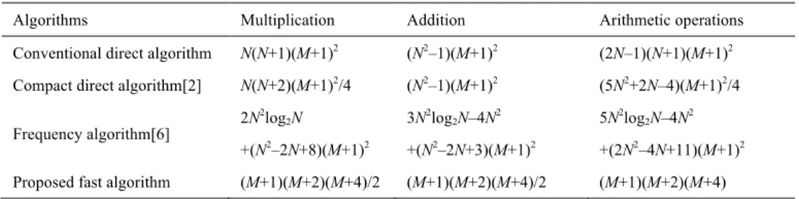
The computational complexities of the four algorithms are depicted in Table 1. It can be observed from this table that: (i) The proposed algorithm is independent of the window length N while this is not the case for the other three algorithms; (ii) the proposed algorithm requires fewer arithmetic operations than the other three algorithms when M is not greater than (3N/2–5). Note that the order M must be smaller than the window length N according to the definition of Tchebichef moments in (2). Now, if we consider the worst case where M = N–1, it appears that (i) the proposed algorithm is superior to the other three algorithms when N > 8 and (ii) the proposed algorithm has the same number of arithmetic operations to the compact direct algorithm when

N = 8.

Table 1 Computational complexity for 1-D SDTMs order up to order M

Algorithms Multiplication Addition Arithmetic operations

Conventional direct

algorithm N(M+1) (N–1)(M+1) (2N–1)(M+1)

Compact direct algorithm[2] N(M+1)/2 (N–1)(M+1) (3N/2–1)(M+1)

Frequency algorithm[6] Nlog2N+(N/2+2)(M+1) 3Nlog2N/2–2N+N(M+1)/2 5Nlog2N/2–2N+(N+2)(M+1)

Proposed fast algorithm (M+1)(M+4)/2 (M+1)(M+4)/2 (M+1)(M+4)

(2) Computation of 2-D SDTMs

In this section, we turn to the analysis of 2-D SDTMs and we provide the computational complexity of moments up to order (M, M) for a sliding block of size N " N.

For the conventional direct algorithm, (10) can be rewritten as

1 1 1, , 0 0

( )

(

1 ,

) ( )

N N p q n m n m x y

T

+ !

t x

!

f p

x q y t y

= =

=

"

+ +

+

, 0 ! n, m ! M. (28) Then, the computational complexity is N(N+1)(M+1)2_{multiplications and (N}2_–1)(M+1)2_{additions, while it is decreased to}

N(N+2)(M+1)2_{/4 multiplications and (N}2_–1)(M+1)2_{additions for the compact direct algorithm given by}

/2 1 /2 1 1, , 0 0

(

1 ,

) ( 1) (

1 ,

1 )

( )

( 1) (

,

) ( 1)

(

,

1 )

m N N p q n m n m _n _{m n} x y

f p

x q y

f p

x q N

y

T

t x

t y

f p N x q y

f p N x q N

y

! ! + + = =

"

+ +

+ + !

+ +

+ ! !

#

=

_$

_%

+ !

+ + !

+ !

+ ! !

$

%

&

'

(

, 0 ! n, m ! M. (29)

(8)

(i) the computation of the matrix between the bracket requires (M+1)2_{multiplications and (M+1)}2_{additions; (ii) the}

multiplication of the upper anti-triangular matrix gotten in the bracket by the lower triangular matrix A_M!1 needs M(M+1)2_/2

multiplications and M(M+1)2_{/2 additions; (iii) the remaining operations in (20) or (24) still require (M+1)}2_{multiplications and}

(M+1)2_{additions; (iv) the computation of 1-D horizontal SDTMs in (20) or 1-D vertical SDTMs in (24) using the proposed fast}

algorithm for 1-D SDTMs needs (M+1)(M+4)/2 multiplications and (M+1)(M+4)/2 additions. Thus, the total computational complexity is (M+1)(M+2)(M+4)/2 multiplications and (M+1)(M+2)(M+4)/2 additions.

Table 2 summarizes the computational complexities of the four algorithms. We can draw similar conclusions as 1-D SDTMs from Table 2. Moreover, when compared to 1-D SDTMs, the proposed algorithm for 2-D SDTMs is more efficient than the other three algorithms, even for the worst case where M = N–1 as far as N " 3. In fact, there are few cases in real applications with N < 4. Since the proposed algorithm is independent of the block size, it is very suitable for applications which need to traverse the whole image using a block-based method, such as image forensics, pattern matching and texture analysis and so on.

Table 2 Computational complexity for 2-D SDTMs up to order (M, M)

Algorithms Multiplication Addition Arithmetic operations

Conventional direct algorithm N(N+1)(M+1)2 _(N2_–1)(M+1)2 _{(2N–1)(N+1)(M+1)}2

Compact direct algorithm[2] N(N+2)(M+1)2_/4 _(N2_–1)(M+1)2 _(5N2_{+2N–4)(M+1)}2_/4

Frequency algorithm[6] 2N 2_log 2N +(N2_{–2N+8)(M+1)}2 3N2_log 2N–4N2 +(N2_{–2N+3)(M+1)}2 5N2_log 2N–4N2 +(2N2_{–4N+11)(M+1)}2

Proposed fast algorithm (M+1)(M+2)(M+4)/2 (M+1)(M+2)(M+4)/2 (M+1)(M+2)(M+4)

IV. PERFORMANCE TEST AND APPLICATION

In this section, we first evaluate the performance of the proposed fast algorithm for SDTMs through a comparison of their computational time and we then consider its application in tampering detection. These tests were implemented in VS2010 on a ThinkPad notebook E420 with 2.40 GHz CPU and 4GB RAM.

A. Test of the fast SDTMs in terms of computational time

(1) 1-D SDTMs

In order to evaluate the performance of the proposed fast algorithm for 1-D SDTMs, ten signals (each with 100000 samples) were randomly generated. The values of these ten signals were normalized to the range [–1, 1].

In the first experiment, the 1-D SDTMs of the ten signals were respectively computed using the aforementioned three algorithms. Considering our next targeted applications of 1-D SDTMs in audio signal, the window length N and the maximum order M were respectively set to 16 and 5. Table 3 presents their respective computational time. It can be observed from this table that: (i) our proposed algorithm is faster than the three others; (ii) the computation time remains stable whatever the signal used.

Table 3 Computational time (millisecond) of different algorithms for the ten randomly generated signals (No.1-No. 10)

Algorithms 1 2 3 4 5 6 7 8 9 10

Conventional direct algorithm 32 32 31 32 32 31 32 32 32 33

Compact direct algorithm[2] 26 26 25 25 26 26 26 27 26 27

Frequency algorithm[6] 35 37 35 36 35 35 36 37 37 36

Proposed fast algorithm 15 16 14 15 15 15 15 16 16 15

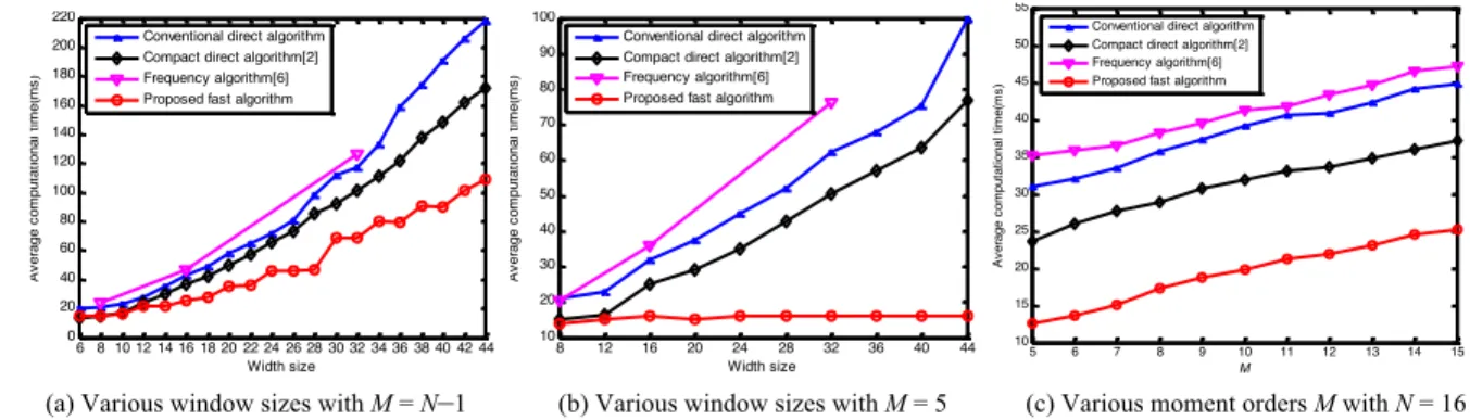
The objective of the second experiment is to evaluate the influence of the window size and of the moment order for the four algorithms. We used the same ten signals. In order to test the influence of the window size, two cases were considered: a) the window size N was varied from 6 to 44 with an increment of 2 and the corresponding order was set to M = N–1, which is the worst case of the proposed algorithm; b) the window size N was varied from 8 to 44 with an increment of 4 using a fixed order set to M = 5, which is the order used in the two applications that will be described later. In order to test the influence of moment

(9)

order, the maximum order M was varied from 5 to 15 and the window size N is 16. Fig. 1 shows the average computational time for the ten signals. Note that Fig.1 (a) and (b) only shows the results of the frequency algorithm for the window sizes equalling to the power of 2 due to the radix-2 FFT algorithm. For other window sizes, zero padding can be applied but at the cost of an increased complexity: let N be the length of the original signal. If 2k_{< N < 2}k+1_{, where k is a positive integer, the complexity for}

the signal after zero padding will be equal to that for the signal with the length 2k+1_{. It can be observed from Fig. 1 that: (i)}

regarding to the window size, the proposed algorithm, although considered in the worst case (M = N–1), leads to a better performance; (ii) when a fixed order M = 5 is considered, the computational time of the proposed algorithm is independent of the window size. However, it is not the case for the other three algorithms, whose computational load increases at a fast rate. It is in agreement with the computational complexity shown in Table 1; (iii) although the computational time of the proposed algorithm increases with the moment orders, the advantage of the proposed algorithm over the direct algorithms and frequency algorithm is evident. This is also consistent with the computational complexity analysis.

6 8 10 12 14 16 18 20 22 24 26 28 30 32 34 36 38 40 42 44 0 20 40 60 80 100 120 140 160 180 200 220 Width size Av er age c om put at ional ti m e( m s)

Conventional direct algorithm Compact direct algorithm[2] Frequency algorithm[6] Proposed fast algorithm

8 12 16 20 24 28 32 36 40 44 10 20 30 40 50 60 70 80 90 100 Width size Av er age c om put at ional ti m e( m s)

5 6 7 8 9 10 11 12 13 14 15 10 15 20 25 30 35 40 45 50 55 M Av er age c om put at ional ti m e( m s)

(a) Various window sizes with M = N–1 (b) Various window sizes with M = 5 (c) Various moment orders M with N = 16 Fig. 1 Average computational time (millisecond) for the different algorithms with various window sizes N and maximum moment orders M

(2) 2-D SDTMs

In order to test the efficiency of the proposed fast algorithm for 2-D SDTMs, considering the following application of 2-D SDTMs in image tampering detection, a set of six tampered images shown in Fig. 2 (a), (c), (e), (g), (i) and (k) has been chosen from the public image manipulation dataset [12]. The sizes of the six images are 504"760.

Fig. 2 Eight tampered images (first and third columns) and their corresponding source images (second and fourth columns) from the public image manipulation dataset. (a) and (k) are plain copy-move forgery. (c), (e), (g), (i), (m) and (o) are the forgery combined with adding Gaussian noise (standard deviation is 0.1), JPEG compression (quality factor is 50), rotation (angle is 10 degree), scaling (factor is 109%), rotation (angle is 6 degree), and scaling (factor

is 91%), respectively.

(10)

packages, especially in Matlab, and they proposed a matrix-based implementation method to compute the Tchebichef moments. So, in this subsection, the proposed fast algorithm is compared with the two direct algorithms presented in Section III.C implemented in VS2010 as well as their matrix-based implementation in MATLAB R2006b. Note that the matrix-based implementation does not change the computational complexity.

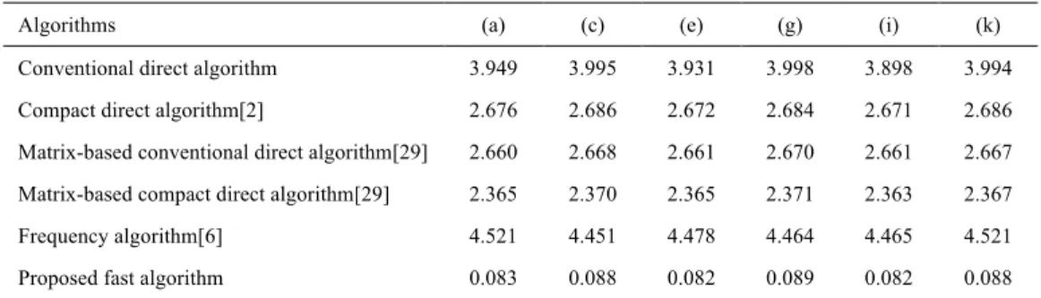
In the first example, the SDTMs of the above six images were respectively calculated by using these different implementations. The block size was set to 16"16 and the maximum order of moments to 5, which is the same one used in [12] for Zernike moments. The resulting computational time is shown in Table 4. Although the matrix-based scheme leads to a significant benefit, it is far from the performance of our proposed algorithm.

Table 4 Computational time (second) of different algorithms for images shown in Fig.2

Algorithms (a) (c) (e) (g) (i) (k)

Conventional direct algorithm 3.949 3.995 3.931 3.998 3.898 3.994

Compact direct algorithm[2] 2.676 2.686 2.672 2.684 2.671 2.686

Matrix-based conventional direct algorithm[29] 2.660 2.668 2.661 2.670 2.661 2.667 Matrix-based compact direct algorithm[29] 2.365 2.370 2.365 2.371 2.363 2.367

Frequency algorithm[6] 4.521 4.451 4.478 4.464 4.465 4.521

Proposed fast algorithm 0.083 0.088 0.082 0.089 0.082 0.088

In the second experiment, we evaluated the influence of block size, moment order, and image size. The six images used in the previous experiment were considered again. For the first test (i.e. influence of block size), two case were examined: (i) the block size N#N was varied from 6#6 to 44#44 with an increment of 2 and the maximum order (M, M) was set to (N–1, N–1) in all cases; (ii) the block size was varied from 8#8 to 80#80 with an increment of 8 and the order was set to (5, 5). For the second test, the block size was set to 16"16 and the maximum order of moments (M, M) was varied from (5, 5) to (15, 15). For the third test, the block size was still fixed at 16"16, the order of moments was chosen equal to (5, 5), and then the six images were rescaled with a factor ranging from 0.5 to 2.1 with step 0.2. The results of the average computational times of these tests are respectively given in Fig. 3. Note that, the same as 1-D SDTMs, Fig. 3 (a) and (b) only shows the results of the frequency algorithm for the block size equalling to the power of 2 owing to the radix-2 FFT algorithm used. It can be seen from these figures that: (i) conclusions similar to those obtained through the previous experiment of 1-D SDTMs can be drawn; (ii) moreover, when compared to 1-D SDTMs, a greater advantage of the proposed fast algorithm over the other algorithms for 2-D SDTMs can be noticed. 6 8 10 12 14 16 18 20 22 24 26 28 30 32 34 36 38 40 42 44 0 50 100 150 200 250 300 350 400 450 500 550 600 650 Width of block Av er age c om put at ional ti m e( s)

Conventional direct algorithm Compact direct algorithm[2]

Matrix-based conventional direct algorithm[29] Matrix-based compact direct algorithm[29] Frequency algorithm[6]

Proposed fast algorithm

08 16 24 32 40 48 56 64 72 80 5 10 15 20 25 30 35 40 45 50 55 60 65 70 75 80 Width of block Av er age c om put at ional ti m e( s)

(11)

5 6 7 8 9 10 11 12 13 14 15 0 3 6 9 12 15 18 21 24 27 M Av er age c om put at ional ti m e( s)

0.5 0.7 0.9 1.1 1.3 1.5 1.7 1.9 2.1 0 5 10 15 20 25 Scaling factor Av er age c om put at ional ti m e( s)

(c) Various moment orders (M, M) with N = 16 (d) Various image sizes with N = 16 and M = 5 Fig. 3 Average computational time (second) for the different algorithms with various block sizes N!N and maximum moment orders (M, M)

Although the proposed algorithm is computationally efficient, it suffers from the problem of accumulated errors, which also exists for the fast computation of other sliding transforms, for example the sliding DFT [23]. For the SDTMs, the accumulated errors are introduced by the iterative updated equations (18), (20) and (24) on each sliding window and two matrices AM and BM

in these equations. These two matrices must be calculated recursively, involving matrix multiplication and truncation and so leading to several sources of numerical approximation. In fact, if AM and BM are calculated in double precision, the accumulated

errors remain small as it will be shown below. If one wants to further reduce the accumulated errors, the application of the proposed fast algorithm can be slightly modified by reinitializing the process at some regular interval K (the procedure is restarted from the step 3) depicted in Section III.B). The following experiment was carried out to better quantify these accumulated errors.

For the six tampered images of size 504"760 considered in the previous subsection, we computed the SDTMs on 364305 (=(504–15)"(760–15)) blocks of size 16"16 for each image by using different values of the interval K. The definition of the relative errors between SDTMs can be found in [30]. The experimental results are provided in Table 5. They show that: (i) the modified algorithm allows reducing the accumulated errors from e-7 to e-14; (ii) however, the initial proposed algorithm with no interval leads also to small errors (lower than 2.56e-7).

Table 5 Maximum relative error over 364305 blocks for different images using various K

K Fig.2(a) Fig.2(c) Fig.2(e) Fig.2(g) Fig.2(i) Fig.2(k)

50 5.43e-14 1.04e-13 1.49e-13 4.03e-14 9.96e-14 1.36e-13

100 1.83e-13 1.07e-13 3.07e-13 6.87e-14 1.14e-13 1.83e-13

150 3.25e-13 1.87e-13 4.03e-13 1.19e-13 3.20e-13 4.50e-13

200 1.93e-12 6.41e-13 8.28e-13 8.93e-13 2.65e-12 1.31e-12

250 1.80e-11 4.85e-12 3.60e-11 7.89e-12 2.03e-11 8.47e-12

300 5.32e-11 2.52e-11 3.69e-10 5.05e-11 5.23e-11 6.12e-11

350 3.32e-10 1.50e-10 1.36e-9 3.59e-10 3.72e-10 4.60e-10

400 5.23e-10 6.43e-10 2.41e-9 1.00e-9 3.05e-9 2.35e-9

450 1.51e-9 2.95e-9 2.39e-9 1.68e-9 7.73e-9 1.32e-8

500 4.37e-9 6.63e-9 3.55e-9 7.40e-9 2.34e-8 3.61e-8

No interval 1.13e-7 7.11e-8 2.45e-7 6.10e-8 3.79e-8 2.56e-7

B. Application of SDTMs to duplicated signal segments and image regions detection

As a kind of sliding orthogonal transform, SDTMs can be used to the same applications in signal processing as other sliding transforms, such as signal filtering, spectrum analysis, matching, and tampering detection. Here, tampering detection, more precisely the detection of duplicated signal segments in an audio wave or regions in an image, is considered. The general pipeline for copy-move forgery detection (CMFD) provided in [12] will be closely followed in our application examples.

(12)

With the rapid development of low cost and sophisticated image processing software tools, digital images can be tampered easily with no obvious visual traces. Copy-move manipulations, a common form of local processing, copy parts of an image and paste them somewhere else in the same image [31]. Therefore, automatic detection of duplicated regions is becoming one of the most important and popular digital forensic techniques currently [32]. In [12], Christlein et al. provided a general pipeline for blind passive CMFD without using source images shown in Fig. 4.

Pre-processing ExtractionFeature Matching Filtering processing

Post-Keypoint Detection Block Tiling

Fig. 4 General processing pipeline for the region duplication forgery detection using the keypoint-based features or the block-based ones [12].

The detailed steps for block-based methods are as follows: 1) Convert the color image to gray image;

2) Subdivide the test image into overlapping blocks of size N"N; 3) Compute a feature vector for every block;

4) Match each feature vector by searching its nearest one with the minimum Euclidean distance in the feature domain using kd-tree matching;

5) Remove the matched block pairs that are spatially close to each other, i.e. ₁

2

ij v <

!

!!"

, where v!!"_ij is the translation difference (“shift vector”) between the matched blocks i and j, and !₂ is the Euclidean norm;

6) Cluster the remaining pairs that adhere to a joint pattern. Let P(A) be the number of pairs satisfying the same affine transformation T. Remove all pairs that belong to a small number P(A), i.e. P(A) <

"

2;

7) Preserve the connected regions with the number of pixels more than

"

3 and highlight them with bright color as tampered

regions.

Christlein et al. [12] have used two objective criteria Recall (or true positive rate) and Precision to evaluate the efficiency of the algorithms for duplicated region detection. Recall represents the probability that a forgery is detected, while Precision shows the probability that a detected forgery is truly forged. These two objective criteria are also used in the following experiments.

(1) Audio signal duplicated segments detection using 1-D SDTMs

Audio forgery techniques could be used to falsify court evidence, conduct piracy over the Internet, or modify security device recordings or recordings of events taking place in different parts of the world. There are many ways to tamper digital audio. The duplicated audio inserting is a common one. For example, suppose that we have several audio wave files corresponding to some sentences. One can identify a segment of audio wave including the word “not” and insert this segment into any sentences to change their meaning [33].

So, in the present experiment, 1-D Tchebichef moments were considered as the feature set for detecting the duplicated segments in the signal. The procedure is similar to the one used in image and described by the steps 1 to 7 above. The differences are as follows: 1) the first step is replaced by a normalization of the signal values between 0 and 1 to deal with the different ranges of audio signal values; 2) the second step consists to subdivide the signal into overlapping N-length segments; 3) our fast method based on 1-D Tchebichef moments is applied in the third step. Note that the detection is also a blind passive one (i.e. the source signal is not used). The parameters N, "1, "2 and "3 have been respectively set as: N = 16,

"

1 = 50,

"

3 =

"

2 = 300. The

maximum order M of 1-D SDTMs has been set to 5.

In order to evaluate the detection performance of the proposed algorithm based on 1-D SDTMs, 100 tampered audio signals were considered with 80 signals randomly selected from the public TIMIT dataset [34] and 20 signals created by us. One or two segments of each source file were copied and pasted somewhere else in the same signal to get the tampered signal. Furthermore,

(13)

to these 100 tampered signals, Gaussian white noise with different standard deviations (STDs) were added and converted into MP3 files with different compression ratios to test the robustness of the proposed algorithm.

We also compared the proposed algorithm with the recent work reported by Xiao et al [33]. In [33], Xiao et al. first defined the similarity between two segments and then used a fast convolution algorithm to calculate the similarity. The same two objective criteria (recall and precision) used in image tampering detection experiments were considered for comparison. The results are provided in Table 6 and Table 7. Two examples of detection are given in Fig. 5 and Fig. 6 for illustration. These two examples correspond to two worst cases of noise attack and MP3 compression attack. The detected duplicated segments are highlighted in black. It can be observed from these tables and figures that: 1) the two algorithms well detect duplicated segments in the attack-free scenario; 2) the proposed algorithm has a better performance than Xiao’s algorithm [33] in case of the attack.

Table 6 Recall and precision for additive Gaussian white noise with different STDs

STD of Gaussian 0 0.001 0.002 0.003 0.004 0.005 0.006 0.007 0.008 0.009 0.01 Recall Xiao’s algorithm[33] 100% 100% 100% 95% 90% 86% 81% 74% 68% 63% 58% Proposed algorithm using 1-D SDTMs 100% 100% 100% 100% 100% 96% 92% 87% 83% 80% 76% Precision Xiao’s algorithm[33] 100% 100% 99% 93% 87% 82% 77% 70% 63% 56% 51% Proposed algorithm using 1-D SDTMs 100% 100% 100% 100% 98% 93% 89% 85% 82% 77% 71%

Table 7 Recall and precision for MP3 compression

Compression ratio (Kbps) 16 24 32 40 48 Recall Xiao’s algorithm[33] 74% 83% 87% 93% 100% Proposed algorithm using 1-D SDTMs 84% 91% 100% 100% 100% Precision Xiao’s algorithm[33] 69% 79% 85% 90% 100% Proposed algorithm using 1-D SDTMs 81% 90% 98% 100% 100% 0 10000 20000 30000 40000 50000 60000 70000 80000 90000 100000 105000 -1 -0.5 0 0.5 1

(a) Original waveform “He is the murder. I am not the murder.”

0 10000 20000 30000 40000 50000 60000 70000 80000 90000 100000 105000 -1 -0.5 0 0.5 1

(b) Tempered waveform “He is not the murder. I am not the murder.”

0 10000 20000 30000 40000 50000 60000 70000 80000 90000 100000 105000 -1 -0.5 0 0.5 1

(c) Tempered waveform without attack and detected results

0 10000 20000 30000 40000 50000 60000 70000 80000 90000 100000 105000 -1 -0.5 0 0.5 1

(d) Tempered waveform under Gaussian noise attack (STD=0.01) and detected results

0 10000 20000 30000 40000 50000 60000 70000 80000 90000 100000 105000 -1 -0.5 0 0.5 1

(14)

Fig. 5 Example of detection in audio signal with duplicated segments. Original waveform: “He is the murder. I am not the murder”. Tampered waveform: “He is not the murder. I am not the murder”.

Fig. 6 Example of detection for an audio signal with duplicated segments. Original waveform: “One two three four five six seven eight nine ten”. Tampered waveform: “One two three four five two seven eight five ten”.

(2) Image duplicated regions detection using 2-D SDTMs

In [12], Christlein et al. compared the performance of 15 most prominent feature sets including the keypoint-based features SIFT and SURF, as well as the block-based ones using discrete cosine transform (DCT), discrete wavelet transform (DWT), principal component analysis (PCA), kernel-PCA (KPCA), Hu’s moment invariants, blur invariant moments and Zernike moments. Experimental results in [12] demonstrate that Zernike moments have on the overall the best performance. So, in this paper, we compared the feature sets based on Tchebichef and Zernike moments under the same CMFD pipeline as [12] given at the beginning of this section IV.B to evaluate the performance of the fast algorithm for 2-D SDTMs.

a) Experimental dataset

To do so, the public image manipulation dataset used in [12] was considered. This dataset contains 48 source images and many snippets manually extracted from these source images. The tampered images are obtained by copying and pasting these snippets into the source images. They cover different levels of sophistication with duplicated regions of varying numbers and sizes. In order to test the robustness, these snippets are also scaled, rotated, noised, or JPEG compressed before being copied and pasted. Some representative tampered images and their corresponding source images are shown in Fig. 2. The tampered regions are marked with red line. Note that the detection of duplicated regions discussed in this section is a blind one (no use of the source image). Here, the source images are only displayed for illustration.

The sizes of the images in this dataset vary from 800"533 to 2613"3900. In our experiments, the images larger than 1440"1440 were down-sampled with a scaling factor equal to 0.25 and the rest with a scale factor of 0.5. The reasons of this pre-processing are the following: (i) we want to accelerate the process of duplicated regions detection according to our PC configuration since a large image leads to a great number of feature vectors to be matched; (ii) the down-sampling does not affect the comparison of the three algorithms here used as shown in the experiments conducted on images of various sizes; (iii) experimental results reported in [12] have shown that the down-sampling leads to a decrease of the overall detection performance. So, here, we have tested attacks combined with down-sampling. These attacks are more complex than those carried out in [12].

0 20000 40000 60000 80000 100000 115000 -1 -0.5 0 0.5 1

(a) Original waveform “One two three four five six seven eight nine ten.”

0 20000 40000 60000 80000 100000 115000 -1 -0.5 0 0.5 1

(b) Tempered waveform “One two three four five two seven eight five ten.”

0 20000 40000 60000 80000 100000 115000 -1 -0.5 0 0.5 1

(c) Tempered waveform without attack and detected results

0 20000 40000 60000 80000 100000 115000 -1 -0.5 0 0.5 1

(d) Tempered waveform under Gaussian noise attack (STD=0.01) and detected results

0 20000 40000 60000 80000 100000 115000 -1 -0.5 0 0.5 1

(15)

Note that due to the down-sampling, the parameters

"

3 and

"

2 were set to 300 instead of 800 for the Zernike moments in [12]. The

other parameters N, "1, and M remained identical as in [12]: N = 16,

"

1 = 50 and M = 5.

b) Experimental results

We compared the proposed algorithm using 2-D SDTMs with two other algorithms. The first one, which is named “Algorithm 1” hereafter, is the algorithm reported in [12], combining the Zernike moment features with a kd-tree matching. The second one, called “Algorithm 2”, also based on Tchebichef moments, was proposed by Li et al. [35] where the moments of every block are computed using the direct algorithm coupled with a lexicographic sorting for matching similar feature vectors.

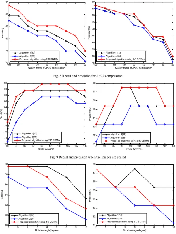
The results are shown in Table 8 and Fig. 7-Fig. 10. They show that:

1) The proposed algorithm, which combines the Tchebichef moments with kd-tree matching, is superior to the other two algorithms in terms of both Recall and Precision, no matter the manipulations done, except for the rotation operations for Algorithm 1 [12]. This is mainly due to the following facts: (i) Tchebichef moment features are superior to Zernike moment features [1-5]; (ii) the kd-tree matching can achieve better results than the lexicographic sorting [12]; (iii) the features used in Algorithm 1 are the magnitudes of the Zernike moments, invariant to rotations;

2) Both criteria decrease when increasing the level of attacks (higher noise, larger compression, etc.) except for few cases; 3) Due to the image down-sampling, the overall performances of all compared algorithms are slightly inferior to the results obtained in [12] when the original full size images are used: both of the Recall and Precision for the plain region duplication forgery is lower than 100%. This behavior has also been observed and pointed out by Christlein et al. in [12](Algorithm 1).

Table 8 Results for plain region duplication forgery (Algorithm 1 is based on Zernike moments and kd-tree matching; Algorithm 2 combines Tchebichef moments and lexicographic sorting; the proposed algorithm uses the fast computation of Tchebichef moments and kd-tree matching)

Algorithms Recall Precision

Algorithm 1[12] 89.6 87.5 Algorithm 2[35] 87.5 85.4 Proposed algorithm using 2-D SDTMs 93.8 87.5 0.02 0.03 0.04 0.05 0.06 0.07 0.08 0.09 0.1 72 74 76 78 80 82 84 86 88 90

Standard deviation of Gaussian noise

Rec al l(% ) Algorithm 1[12] Algorithm 2[35]

Proposed algorithm using 2-D SDTMs

0.02 0.03 0.04 0.05 0.06 0.07 0.08 0.09 0.1 81 82 83 84 85 86 87 88

Standard deviation of Gaussian noise

Pr ec is ion( % ) Algorithm 1[12] Algorithm 2[35]

Fig. 7 Recall and precision for additive Gaussian white noise

(16)

20 30 40 50 60 70 80 90 100 70 75 80 85 90 95

Quality factor of JPEG compression

Rec al l(% ) Algorithm 1[12] Algorithm 2[35]

20 30 40 50 60 70 80 90 100 45 50 55 60 65 70 75 80 85 90

Quality factor of JPEG compression

Pr ec is ion( % ) Algorithm 1[12] Algorithm 2[35]

Fig. 8 Recall and precision for JPEG compression

91 93 95 97 99 101 103 105 107 109 72 74 76 78 80 82 84 86 88 90 92 Scale factor(%) Rec al l(% ) Algorithm 1[12] Algorithm 2[35]

91 93 95 97 99 101 103 105 107 109 81 82 83 84 85 86 87 88 Scale factor(%) Pr ec is ion( % ) Algorithm 1[12] Algorithm 2[35]

Fig. 9 Recall and precision when the images are scaled

2 3 4 5 6 7 8 9 10 78 80 82 84 86 88 90 Rotation angle(degree) Rec al l(% ) Algorithm 1[12] Algorithm 2[35]

2 3 4 5 6 7 8 9 10 81 82 83 84 85 86 87 88 Rotation angle(degree) Pr ec is ion( % ) Algorithm 1[12] Algorithm 2[35]

Fig. 10 Recall and precision for rotation

In order to better apprehend these results, visual examples are provided in Fig. 11. These examples correspond to some of those shown in Fig. 2 in the case of a plain copy-move forgery and four different types of additional manipulations. Detected regions are highlighted by colored areas. It can be seen from this figure that the proposed algorithm can correctly detect duplicated regions though the snippets are processed by some manipulations before being pasted. However, this is not the case for the other algorithms. Indeed, sometimes Algorithm1 and Algorithm 2 fail to detect or localize properly duplicated regions with many false positives detection (see for instance, the sky regions of Fig. 11(g) and (h)).

(17)

Fig. 11 Examples of detected duplicated regions (tampered images shown in Fig. 2). Columns are successively the detected results using Algorithm 1[12], Algorithm 2[35] as well as our algorithm.

V. CONCLUSIONS

In this paper, by establishing the link between the Tchebichef moments of two overlapping windows based on some properties of the Tchebichef polynomials, we have presented a fast computation algorithm for 1-D and 2-D sliding discrete Tchebichef moments. The computational complexity analysis and the experimental results demonstrate that our algorithm is more efficient than the conventional direct ones. A notable difference with the direct algorithm is that the proposed algorithm is independent of the block size and is particularly suitable for applications which need to slide a window over the whole signal or image.

Two pplication examples aimed at the detection of duplicated signal segments and image regions has been developed in order to show the efficiency of our approach. On one hand, we have shown that our 1-D SDTMs algorithm leads to a better performance in audio signal than the algorithm reported by Xiao et al [33]. On the other hand, for image duplicated regions detection, our solution based on 2-D SDTMs is superior to the algorithm based on Zernike moment features and kd-tree technique reported in [12] and the algorithm proposed by Li et al. [35] where the Tchebichef moments of every block are used in combination with a lexicographic technique.

ACKNOWLEDGEMENTS

The authors thank V. Christlein and C. Riess [12] for sharing their code and dataset as well as their helpful suggestions. REFERENCES

[1] R. Mukundan, S.H. Ong, and P.A. Lee, “Image analysis by Tchebichef moments,” IEEE Trans. Image Process., vol. 10, no. 9, pp. 1357-1364, 2001. [2] G.B. Wang and S.G. Wang, “Recursive computation of Tchebichef moment and its inverse transform,” Pattern Recogn., vol. 39, no. 1, pp. 47-56, 2006. [3] H.Z. Shu, H. Zhang, B.J. Chen, et al., “Fast computation of Tchebichef moments for binary and grayscale images,” IEEE Trans. Image Process., vol. 19,

no. 12, pp. 3171-3180, 2010.

[4] B.H.S. Asli, R. Paramesran, and C.L. Lim, “The fast recursive computation of Tchebichef moment and its inverse transform based on Z-transform,”

Digital Signal Process., vol. 23, no. 5, pp. 1738-1746, 2013.

[5] H. Zhang H, X.B. Dai, P. Sun, et al., “Symmetric image recognition by Tchebichef moment invariants,” in: Proc. 2010 17th IEEE Int. Conf. Image

(18)

[6] J.V. Marcos and G. Cristóbal, “Texture classification using discrete Tchebichef moments,” J. Opt. Soc. Am. A, vol. 30, no. 8, pp. 1580-1591, 2013. [7] X.B. Dai, H.Z. Shu, L.M. Luo, et al., “Reconstruction of tomographic images from limited range projections using discrete Radon transform and

Tchebichef moments,” Pattern Recogn., vol. 43, no. 3, pp. 1152-1164, 2010.

[8] H. Huang, G. Coatrieux, H.Z. Shu, et al., “Blind integrity verification of medical images,” IEEE Trans. Inf. Technol. Biomed., vol. 16, no. 6, pp. 1122-1126, 2012.

[9] S.M. Elshoura and D.B. Megherbi, “Analysis of noise sensitivity of Tchebichef and Zernike moments with application to image watermarking,” J. Vis.

Commu. Image R., vol. 24, no. 5, pp. 567-578, 2013.

[10] J. Cao, D.H. Mao, Q. Cai, et al., “A review of object representation based on local features,” J. Zhejiang Univ. SCI. C, vol. 14, no. 7, pp. 495-504, 2013. [11] Z. Chen and S.K. Sun, “A Zernike moment phase-based descriptor for local image representation and matching,” IEEE Trans. Image Process., vol. 19, no.

1, pp. 205-219, 2010.

[12] V. Christlein, C. Riess, J. Jordan, et al., “An evaluation of popular copy-move forgery detection approaches,” IEEE Trans. Inf. Foren. Sec., vol. 7, no. 6, pp. 1841-1854, 2012.

[13] S.J. Ryu, M. Kirchner, M.J. Lee, et al., “Rotation invariant localization of duplicated image regions based on Zernike moments,” IEEE Trans. Inf. Foren.

Sec., vol. 8, no. 8, pp. 1355-1370, 2013.

[14] J.A.R. Macias and A.G. Exposito, “Recursive formulation of short-time discrete trigonometric transforms,” IEEE Trans. Circuits Syst. II: Analog. Digital

Signal Process., vol. 45, no. 4, pp. 525-527, 1998.

[15] V. Kober, “Fast algorithms for the computation of sliding discrete sinusoidal transforms,” IEEE Trans. Signal Process., vol. 52, no. 6, pp. 1704-1710, 2004.

[16] V. Kober, “Fast algorithms for the computation of sliding discrete Hartley transforms,” IEEE Trans. Signal Process., vol. 55, no. 6, pp. 2937-2944, 2007. [17] B. Farhang-Boroujeny and S. Gazor, “Generalized sliding FFT and its application to implementation of block LMS adaptive filters,” IEEE Trans. Signal

Process., vol. 42, no. 3, pp. 532-538, 1994.

[18] C. Park and S. Ko, “The hopping discrete Fourier transform,” IEEE Signal Process. Mag., vol. 31, no. 2, pp. 135-139, 2014.

[19] W.L. Ouyang and W.K. Cham, “Fast algorithm for Walsh Hadamard transform on sliding windows,” IEEE Trans. Pattern. Anal. Mach. Intell., vol. 32, no. 1, pp. 165-171, 2010.

[20] J.A.R. Macias, and A.G. Exposito, “Efficient computation of the running discrete Haar transform,” IEEE Trans. Power Delivery, vol. 21, no. 1, pp. 504-505, 2006.

[21] J.S. Wu, L. Wang, G.Y. Yang, et al., “Sliding conjugate symmetric sequency-ordered complex Hadamard transform: fast algorithm and applications,”

IEEE Trans. Circuits Syst.-I: Regular Papers, vol. 59, no. 6, pp. 1321-1334, 2012.

[22] E. Jacobsen and R. Lyons, “The sliding DFT,” IEEE Signal Process. Mag., vol. 20, no. 2, pp. 74-80, 2003.

[23] K. Duda, “Accurate, guaranteed stable, sliding discrete Fourier transform,” IEEE Signal Process. Mag., vol. 27, no. 6, pp. 124-127, 2010.

[24] R. Tao, Y.L. Li, and Y. Wang, “Short-time fractional Fourier transform and its applications,” IEEE Trans. Signal Process., vol. 58, no. 5, pp. 2568-2580, 2010.

[25] B. Mozafari and M.H. Savoji, “An efficient recursive algorithm and an explicit formula for calculating update vectors of running Walsh-Hadamard transform,” in: Proc. IEEE Int. Conf. Information Sciences, Signal Processing and their Applications, 2007, pp. 1-4.

[26] W.L. Ouyang, R. Zhang, and W.K. Cham, “Fast pattern matching using orthogonal Haar transform,” in: Proc. IEEE CVPR, San Francisco, CA, 2010. pp. 3050-3057.

[27] C.M. Orallo, I. Carugati, and S. Maestri, et al., “Harmonics measurement with a modulated sliding discrete Fourier transform algorithm,” IEEE Trans.

Instrum. Meas., vol. 64, no. 4, pp. 781-793, 2014.

[28] J. Martinez and F. Thomas, “Efficient computation of local geometric moments,” IEEE Trans. Image Process., vol. 11, no. 9, pp. 1102-1111, 2002. [29] P.T. Yap and P. Raveendran, “Image focus measure based on Chebyshev moments,” IEE Proc.-Vision, Image and Signal Process., vol. 151, no. 2, pp.

128-136, 2004.

[30] B.J. Chen, H.Z. Shu, H. Zhang, et al., “Combined invariants to similarity transformation and to blur using orthogonal Zernike moments,” IEEE Trans.

Image Process., vol. 20, no. 2, pp. 345-360, 2011.

(19)

USA, 2003.

[32] J. Li, X.L. Li, B. Yang, et al., “Segmentation-based image copy-move forgery detection scheme,” IEEE Trans. Inf. Foren. Sec., vol. 10, no. 3, pp. 507-518, 2015.

[33] J.N. Xiao, Y.Z. Jia, E.D. Fu, et al., “Audio authenticity: Duplicated audio segment detection in waveform audio file,” J. Shanghai Jiaotong Univ.

(Sci.), vol. 19, no. 4, pp. 392-397, 2014.

[34] J.S. Garofalo, L.F. Lamel, W.M. Fisher, et al., The DARPA TIMIT Acoustic-Phonetic Continuous Speech Corpus CDROM, Linguistic Data Consortium, 1993.

[35] M. Li, Z. Gu, and J. Kan, “Passive digital image authentication algorithm based on Tchebichef moment invariants,” in: Proc. Fourth Int. Seminar Modern

Cutting and Measuring Engineering, 2010, pp. 79972T-79972T-7.

Beijing Chen received the Ph.D. degree in Computer Science in 2011 from Southeast University, Nanjing,

China. Now he is an associate professor in the School of Computer & Software, Nanjing University of Information Science & Technology, Nanjing, China. His research interests include color image processing, information security and pattern recognition.

Gouenou Coatrieux received the Ph. D. degree in signal processing and telecommunication from the

University of Rennes I, Rennes, France, in collaboration with the Ecole Nationale Supérieure des Télécommunications, Paris, France, in 2002. He is currently a professor in the Information and Image Processing Department, Institut Mines-Telecom, Telecom Bretagne, Brest, France, and his research is conducted in the LaTIM Laboratory, INSERM U1101, Brest. His primary research interests concern medical information system security, watermarking, electronic patient records, and healthcare knowledge management.

Jiasong Wu obtained a joint Ph. D. degree of the Southeast University, Nanjing, China, and the University of

Rennes 1, Rennes, France, in 2012. He is now an assistant professor of Southeast University. His research interest is focused on fast algorithms of digital signal processing, compressed sensing and convolutional network.

Zhifang Dong received the Ph.D. degree in Biological Science in 2011 form Southeast University, Nanjing,

China. Now she is an associate professor in the School of Electronic Science and Engineering, Southeast University, Nanjing, China. Her research interest includes signal and image processing.

Jean Louis Coatrieux received the Ph.D. and State Doctorate in Sciences in 1973 and 1983, respectively,

from the University of Rennes 1, Rennes, France. Since 1986, he has been Director of Research at the National Institute for Health and Medical Research (INSERM), France, and since 1993 has been Professor at the New Jersey Institute of Technology, USA. He has been the Head of the Laboratoire Traitement du Signal et de l'Image, INSERM, up to 2003. His experience is related to 3D images, signal processing, computational modeling and complex systems with applications in integrative biomedicine. He published more than 300 papers in journals and conferences and edited many books in these areas. He has served as the Editor-in-Chief of the IEEE Transactions on Biomedical Engineering (1996-2000) and is in the Boards of several journals.

(20)

Huazhong Shu received the B.S. Degree in Applied Mathematics from Wuhan University, China, in 1987,

and a Ph.D. Degree in Numerical Analysis from the University of Rennes (France) in 1992. He is now a professor of the Department of Computer Science and Engineering of Southeast University, China. His recent work concentrates on the image analysis, pattern recognition, and fast algorithms of digital signal processing.