HAL Id: hal-01060114
https://hal.archives-ouvertes.fr/hal-01060114
Submitted on 2 Sep 2014
HAL is a multi-disciplinary open access
archive for the deposit and dissemination of
sci-entific research documents, whether they are
pub-lished or not. The documents may come from
teaching and research institutions in France or
abroad, or from public or private research centers.
L’archive ouverte pluridisciplinaire HAL, est
destinée au dépôt et à la diffusion de documents
scientifiques de niveau recherche, publiés ou non,
émanant des établissements d’enseignement et de
recherche français ou étrangers, des laboratoires
publics ou privés.
New IPv6 Identification Paradigm: Spreading of
Addresses Over Time
Florent Fourcot, Laurent Toutain, Frédéric Cuppens, Nora
Cuppens-Bouhlahia, Stefan Köpsell
To cite this version:
Florent Fourcot, Laurent Toutain, Frédéric Cuppens, Nora Cuppens-Bouhlahia, Stefan Köpsell. New
IPv6 Identification Paradigm: Spreading of Addresses Over Time. ICNS 2014 : the tenth International
Conference on Networking and Services, Apr 2014, Chamonix, France. pp.74 - 83. �hal-01060114�
New IPv6 Identification Paradigm:
Spreading of Addresses Over Time
Florent Fourcot, Laurent Toutain
Fr´ed´eric Cuppens and Nora Cuppens-Boulahia
Institut Mines-T´el´ecom; T´el´ecom Bretagne Universit´e europ´eenne de Bretagne
Email:{first}.{last}@telecom-bretagne.eu
Stefan K¨opsell
TU Dresden; Faculty of Computer Science Email: [email protected]
Abstract—The identification of packet flows is a very important feature to provide security on the Internet. This flow identification is traditionally done by the well-know five tuple source IP address, destination IP address, transport layer protocol number and the two source/destination identifiers of transport layer protocols (named ports on UDP and TCP). Unfortunately, the IP source address is not reliable at all. However, we can use new security paradigms based on new IPv6 properties. In particular, IPv6 introduces a large address space. Our solution takes the benefit of this space with a high frequency rotation of IP addresses, that we call spreading. This spreading improves the security since only the sender and the receiver are able to generate and follow this temporal sequence. An attacker will not be able to successfully insert malicious packets into a flow or to initialize a flow. It protects against session initialization flooding and against attacks on established connections. In this paper, we describe the architecture of our solution and the protocol to initiate a connection and also performance evaluation of our spreading.
Keywords–IPv6; security; flow identification; spoofing.
I. INTRODUCTION A. Flow identification in the current Internet
Flow identification is the base of some Internet mecha-nisms, like security (filtering of packets) and priority policies for Quality of Service. But since the Internet is a datagram network and IP is not a connection oriented protocol, the notion of flow is not explicit at the network layer. Each packet is independent, and two similar packets can follow two different routes. It is why a flow is defined in the RFC 2722 [1] as “an artificial logical equivalent to a call or connection”. It is “artificial”, and there are no easy ways to discriminate a flow in an IP network.
At the transport layer, the concept of flow is more natural. This is a mandatory function to sort packets, reassemble seg-ments and detect errors, like the popular protocol Transmission Control Protocol (TCP) [2] does. To have this notion of flow, one can use Transport Layer addresses, named ports in case of TCP.
This is why we need a tuple of five elements in order to extract the notion of flow on the network. The first two are the source’s and destination’s IP addresses, directly available in the IP headers. The next one is the transport layer number, avail-able in the field next header for a Internet Protocol version 6 (IPv6) packet without extensions. With the knowledge of the transport protocol, it is possible to parse the transport header
and also to read the port numbers. They complete the tuple, already filled with the three identifiers of IP header.
This well known five tuple is the basic identification of a flow. The identification can be more complex. For example, a stateful firewall will follow the TCP states of each connection, and it will discard packets if they do not follow the TCP standard.
B. Address spreading benefits
These five members of the identification tuple
(IPsrc, IPdst, N extHeader, P ortsrc, P ortdst) are not
authentic by nature. The source IP address and the source port especially can be manipulated easily by an attacker. If an attacker is able to send packets with a spoofed source IP address, he will be in good position to try TCP reset attacks, to inject packets on the destination network, to try a targeted attack to the destination, etc.
With IPv6, the large IP address space allows new secu-rity opportunities, like Cryptographically Generated Address (CGA) [3]. If all IPv4 solutions had to minimize the number of IP addresses in use, it is now possible to use a lot of addresses. Our solution provides security thanks to the spreading of addresses. In our solution, source and destination IP addresses of a flow are renewed frequently, according to a temporal sequence. If this sequence is known only by the sender and the receiver, it adds a new identification feature.
Since we only modify IP addresses, our solution is pretty simple. It does not need some complex encapsulation (like IPsec tunnel does), and can be followed by a firewall with the knowledge of a shared secret.
C. Attacker model
Our attacker can inject some traffic with a spoofed source IP address. He can be on the transmission path and also able to read the legitimate traffic.
We do not try to protect against a rebuilding of a flow. This means that the attacker can use upper layers information like TCP ports and sequence numbers to rebuild the real flow. Our protection is against the spoofing: our spreader will recognize packets from the attacker. However, we provide a protection against correlation of flows, since we obfuscate addresses. An attacker can not guess the real source and destination addresses of a flow, and can not group several flows to one source or destination just with the help of the information available at the network layer.
routing interface
prefix indentifier
+---+---+
| n bits | 128-n bits |
+---+---+
Figure 1: The two parts of IPv6 addresses
D. The two IPv6 address parts
An IPv6 address is divided in two parts, depicted in Figure 1. The routing part (usually called “prefix”) is not rewritable without connectivity issues, since such modification on the destination address will prevent upstream routers to send packets to the destination. In the same way, the source address has to be compliant with the anti-spoofing rules of the RFC 2827 [4] and could not be arbitrary rewritten.
There is no recommended size of prefix for a end network [5], but the length can not be more than 64 bits for compatibil-ity with the IPv6 autoconfiguration. Indeed, the IPv6 Stateless Address Autoconfiguration (SLAAC) derives the second part of the address (named interface identifier) from the hardware MAC address to an identifier of 64 bits. A prefix larger than 64 bits breaks this autoconfiguration.
We choose to rewrite only the last 64 bits of each address, giving a total of 128 bits. Since 64 bits is the maximum size for a prefix compatible with autoconfiguration, this value will be compatible with almost all networks.
E. Related work
There is some previous work on dynamical IPv6 addresses. The nearest of our work is the “Moving target IPv6 Defense” publication [6]. This solution uses an User Datagram Protocol (UDP) tunnel to often rotate addresses and to encapsulate the real IP packet. An encryption is optional to protect the payload of the packet. The main drawback of this paper is the choice to make an encapsulation. It means that the solution has to fragment big packets to prevents Maximum Transmission Unit (MTU) problems and to reassemble it at the end of the tunnel. On the other hand, additional headers can have a bandwidth performance impact. This proposition does not use a temporal window for old address to prevent false positive.
An other idea is the publication “An Architecture for Network Layer Privacy” [7]. It uses an Site Multihoming by IPv6 Intermediation (SHIM6) extension to spread addresses over time. Since SHIM6 is an end-to-end solution, the end device has to allocate all possible addresses before using the connection. It is probably not desirable that a computer allocates 1000 addresses on one network interface, because it will send a lot of Neighbor Discovery packet.
An other paper [8] uses SHIM6 for a protection against deny of services. The idea is to switch from an address (under attack) to another one (not under attacks) for all connections already established.
F. Organization of this paper
In this paper, we first presents some problems of address spreading and our solution of architecture to overcome them
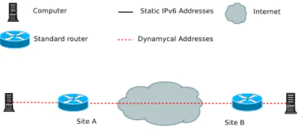
Figure 2: Spreading of addresses without extra device
in Section II. Second, we introduce principles of the spreading and some notations in Section III. We describe step by step the initialization of a connection in Section IV, that we com-plete with a description of packet processing on spreaders in Section V. We introduce the theoretical source of performance issues in Section VI. We close the paper with the description of performance evaluation in Section VII.
II. LOCALIZATION OF THE SPREADER A. Difficulties to spread addresses on the end devices
The first idea of spreading is to generate and follow the address sequence on the end devices (see Figure 2). This strategy allows a end-to-end security, and the computer does not need to delegate the security to someone.
However, this solution implies an upgrade of the local router. The main issue arises if the end device does not get a delegated prefix, but share the local prefix with several end devices. The use of a lot of addresses will:
• flood the network with Neighbor Discovery packets.
The router is not aware of the spreading, and can not know the link between the temporal sequence of IP addresses and the static MAC address;
• saturate the Neighbor table of the router. With
fre-quently switching of addresses, the router will not be able to store all mappings between IP addresses and MAC addresses;
• introduce a latency at each IP address switching, due
to the Neighbor Discovery.
To solve these issues, a solution is to patch the router to follow the sequence of IP destination addresses in the Neighbor table. Thus, the router does not need to know the sequence of source addresses received from the Internet, and is not able to insert a packet in a flow.
B. The prefix delegation solution
With IPv6, we could have enough addresses to delegate one address prefix to each end device. It solves the problem of the mapping between MAC addresses and IP addresses, since the intermediate only send all IP packets matching a prefix to a MAC address.
In this case, the end device is in charge of Interface Identifiers management and can actually be seen as a “router”, and it is the same architecture at the network layer shown in Figure 3. The delegation of address prefixes is the best
Figure 3: Architecture of the solution: spreader on the border of the local network
Figure 4: Architecture of the solution: spreader at the border of the trusted zone
architecture for the simplicity of the solution and from a security point of view. However, we need to provide a solution for a standard network without delegation of prefixes.
C. Simplification with a spreader on the path
For a first approach, we propose to simplify the problem by adding some new “spreaders”, devices on the path of the communication. These devices are able to rewrite a flow of packets with stable addresses to a flow of packet with dynamical addresses. The spreader can be directly on the border of the network (see Figure 3) or at the border of the trusted zone (see Figure 4).
The first positive argument for this architecture is the simplicity to deploy the solution. An administrator does not need to upgrade and configure each end device, but can simply insert the spreader in the network. It has the same benefit than a modified router following the relation between IP and MAC address, and less drawback.
The second point is the ability of bad packets filtering. Since malicious packets consume resources, and can be send to simply saturate the bandwidth of the network, we have to discriminate malicious packets as soon as possible. With an introduction of the spreader at the border of the trust zone, we achieve efficiently this goal.
We choose this architecture for this paper to simplify concepts and experimentations.
III. GENERAL PRINCIPLES A. Prerequisite of the solution
To enable the spreading, we need at least to configure two networks, for the mapping between the dynamical addresses
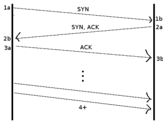
Figure 5: Digital timing diagram of a connection initialization
and stable identifiers.
This configuration is done by adding one spreader at the border of each network. The two spreaders have to share a secret, that an attacker can not guess. The communication of this secret is out-of-scope of this paper.
B. Initialization of the spreader
The initialization of the spreader has to create a config-uration for each compatible peer with a shared secret. This configuration contains the prefix list of the destination (to catch packets to be rewritten) and a function to derive cryptographic keys from the shared secret.
C. Exchange of session data
One of our goals is to spread each flow of data with a unique sequence of addresses, make it more difficult for an attacker to group all flows of one end device. To provide it, both spreaders have to exchange session data at each flow initialization. There are several ways to accomplish it. The first one is to add several extras packets to initiate a context for each flow. It increases latency of connection initialization, and costs some bandwidth.
The second one is to add extra information on a real packet, like by adding one extra IPv6 extension header. Since this extension will be added by the spreader and not by the end devices, it could result in some maximal transport unit problem. Indeed, we can not add this header on a big packet, and have two choices. The first one is to fragment the packet on the spreader, IPv6 RFCs do not allow this solution. The second one is to send a “too big” error to the end devices, which reduce the performance of all packets for the session.
These solutions are not satisfying. We choose another one, our spreaders encode all information in IPv6 source and destination addresses, and do not add any extra data to packets payload. It limits the amount of exchangeable data, but does not have any cost of bandwidth or latency due to extra packets.
D. Notations
The description of the protocol follows the same steps than a TCP connection initialization, depicted in Figure 5.
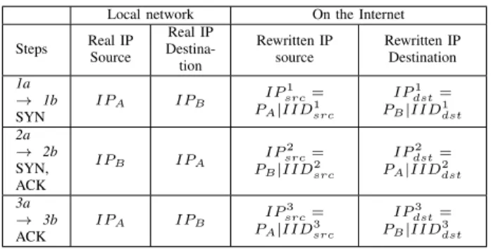
We introduce the following notation for the packet
rewrit-ing (summarized in Table I): PA and PB are the prefixes
of networks for hosts A and B. IPA and IPB are the real
IP addresses of host A and B, concatenation of prefixes and
interface identifiers IIDA and IIDB. IPsrcn is the rewritten
source IP address of the packet in step n, and IPn
dst the
destination IP address in the same step. Since we can not
rewrite the prefixes, IPn
src and IPdstn are concatenation of one
stable prefix (PA or PB) and one rewritten value.
TABLE I: IP ADDRESSES NOTATION
Local network On the Internet Steps Real IP Source Real IP Destina-tion Rewritten IP source Rewritten IP Destination 1a → 1b SYN IPA IPB IP 1 src= PA|IID1src IP1 dst= PB|IIDdst1 2a → 2b SYN, ACK IPB IPA IP 2 src= PB|IID 2 src IP2 dst= PA|IID 2 dst 3a → 3b ACK IPA IPB IP 3 src= PA|IID3src IP3 dst= PB|IIDdst3
IV. STEP BY STEP INITIALIZATION A. Initialization of a connection - first packet
1) Symmetrical rewrite on spreaders: The rewriting begins with step 1a, when the spreader receives a packet with an destination IP address matching one of the prefix in the spreader configuration.
At the first packet of a connection, the local spreader computes new source and destination IP addresses with the help of a cryptographic function. We choose the Advanced Encryption Standard (AES) encryption, but it could be another one allowing encryption of blocks length of 128 bits.
The AES function takes as input a block of both interface identifiers of hosts A and B, and the actual key K(t) derived from the shared secret for the encryption. This AES function has an output of 128 bits, that the spreader divides in two
blocks of 64 bits to replace last 64 bits of IPA and IPB.
IIDsrc1 = AES(IIDA|IIDB, K(t))[0 − 63] (1)
IID1dst= AES(IIDA|IIDB, K(t))[64 − 127] (2)
After the rewriting of addresses, the packet follows the stan-dard routing and filtering process. This ends step 1a.
On the destination spreader, stable addresses are recom-puted in the same way (AES is a symmetric function) in the step 1b. After the computing, the destination spreader checks the validity of the transport layer checksum (this checksum is mandatory for UDP and TCP with IPv6). If the checksum is valid, the packet follows the standard policy of routing and filtering.
If the checksum value is not valid, it can of course be a sign of transmission problem. One other possible cause of this invalid checksum is a try of an attacker to inject one packet in the network, with a spoofing of the source address. Indeed, IPv6 addresses are part of the checksum computation and if addresses after the second spreader are not the same than
addresses sent by the source device, it invalids the checksum. Since the attacker does not know the shared secret, he can not compute the AES encryption and the generated packet will be detected by the spreader.
In more details, the Table II depicts the status of the checksum around the Internet. It looks invalid between the two spreaders, but this is not a problem since nobody needs to have a look on the checksum in the path of the communication. On the contrary, we see in Table III that the checksum of a spoofed packet looks valid on the Internet, but invalid after the rewriting of the second spreader.
TABLE II: CHECKSUM VALIDITY FOR A REAL PACKET
Position Checksum
validity Remarks Local Network Valid Computed by the end device Internet Invalid Addresses have been rewritten, it
invalids the checksum Remote
Network Valid
Addresses have been rewritten by the second spreader
TABLE III: CHECKSUM VALIDITY - SPOOFED PACKET
Position Checksum
validity Remarks Attacker’s
Network Valid Computed by the attacker Internet Valid No rewriting if the attacker is not
aware of protection Remote
Network Invalid
Addresses have been rewritten by the second spreader
2) Security analyze of the rewriting: If the attacker is aware of this spoofing protection, he can try to guess the checksum modification added by the AES encryption of spreaders. The length of the checksum field is 16 bits, which it gives one chance on 65 536 to find the good one. This value is only valid for a short time and for a given address couple, the next
value of K(t) at t+1 will give another checksum modification
implied by the AES encryption.
This security mechanism is not good enough to filter all packets of an attacker, and some packets can bypass this protection. But it is important to notice that if the checksum is valid, the attacker can not guess the rewritten addresses and can not know what is the rewritten destination address. The chance to successfully contact a real computer with a valid address is very low. Indeed, if we assume that the rewriting is fully random, an attacker has first to bypass the checksum (one chance on 65 536). If the checksum is valid, a targeted attack on a computer with an address on the remote network
has one chance on 264 to reach the targeted computer, since
an attacker can not guess the rewritten value after the AES decryption.
B. Initialization of the connection - reply of the remote
The goal of the addresses rewriting on the first packet is to protect an initialization of a connection by an attacker. For the
TABLE IV: REWRITING IN INITIALIZATION STEPS
Steps Rewritten IID Source Rewritten IID Destination
1a → 1b SYN IID1 src= AES(IIDA|IIDB, K(t))[0 − 63] IID1 dst= AES(IIDA|IIDB, K(t))[64 − 127] 2a → 2b SYN, ACK IID2 src= random() IID2 dst= g(t, secret, IID1 src) 3a → 3b ACK IID3 src= g(t, secret, IID1 src) IID3 dst= g(t, secret, IID2 src)
next packets, we create a pseudo-random sequence for each flow of data, generated by a function g. This function g is a generator of a random temporal sequence, one example is a hash function like SHA1.
This creation begins in step 2a. To accomplish it, the second spreader rewrites the first reply packet of a client with a random value as IP source, and a value computed from the source IP address value in the first packet for the destination.
IIDsrc2 = random() (3)
IIDdst2 = g(t, secret, IIDsrc1 ) (4)
g takes as input the current time, the shared secret between networks and another value with the same size than an IP address. This rewriting introduces a random value for the sequence, but the flow is still easy to identify for both spreaders with the IP address destination sets to a value that the first spreader can recognize.
In step 2b, the first spreader recognizes the IP destination
address IPdst2 with the help of a context previously stored.
This packet is an acknowledgment of the initialization, the spreading can now really begin. The spreader saves the value of the IP source (randomized in step 2a) and rewrites the source and destination IP addresses to the real stable value stored in the context.
It ends the second step. The first spreader is now sure of the initialization of the connection, and can use the random value to bootstrap a new random sequence.
C. Initialization of the connection - Acknowledgment of the second spreader
The step 3a begins at the next packet sent by the device from the first network. Both source address and destination address are now spread with:
IID3src= g(t, secret, IID1src) (5)
IID3dst= g(t, secret, IID2src) (6)
In step 3b, the second spreader recognizes the couple with the help of the stored context. This packet is an acknowledgment of the random value send in step 2a, and the second spreader is now aware of the success of the initialization. Steps of initialization are summarized in Table IV.
D. Rewriting during the life of the connection
After the step 3b, both spreaders follow the same
sequence of rewriting with g(t, secret, IID1
src) and
g(t, secret, IID2
src). The rewriting is symmetrical and
both end devices receive stable addresses. An attacker can not inject some traffic since he does not have the knowledge of the next addresses in use.
E. Definition of a flow, division of connections in several temporal sequences
Our goal is to create one sequence of address for each flow of data. By flow, we mean a sequence of packets where informations of upper layers are enough for an attacker to correlate and to rebuild the sequence.
The first trivial idea is to make one flow for each couple
of IPsrc, IPdst. It does not take a lot of resources, but do not
prevent correlation if more than one flow are send between devices. Nevertheless, it can be desirable to obfuscate this information.
IPv6 introduces a new header field to give information about a flow of packets: the flow label field [9]. It is a 20 bits header, that can be used for Quality of Service or other usages (the RFC 6294 [10] tries to give of survey of usages). This flow label can be rewritten on the path of the communication, and is not part of the checksum. Other usages than Quality of Service are allowed, which means that we respect standard specifications [9] with our proposition.
This is why we define a flow by a tuple of
(IPsrc, IPdst, f lowlabel). If the end device set a different
value for two flows, it will be spread into two different sequences. The flow label is set by the end device itself, which has enough information to know if a sequence of packets should not be grouped with another connection.
V. DETAILED PROCESSING ON SPREADERS
Our description of the protocol in Section IV is the ideal situation. We do not have any loss of packets, and the end devices use the TCP protocol. It helps to understand how our protocol works, since it follows the same handshake mechanism than TCP.
But we have to be robust against loss of packets and retransmission of data. In the same way, we have to be com-patible with transport protocols, like UDP, where a connection does not follow a rigorous initialization procedure, or ICMP with short session like a simple Echo request. We detail in this section the processing of packets in spreaders, which actually support loss of packets and is transport layer protocol independent.
A. Detailed steps of packets processing (outgoing packets)
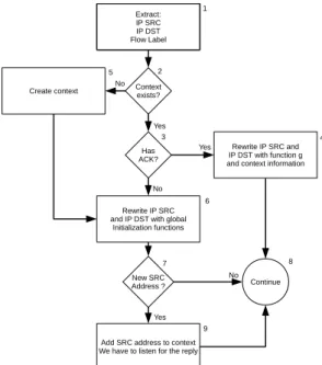
The processing of packets from the local network to the Internet is depicted in Figure 6. For each outgoing packet, the
spreader extracts the tuple (IPsrc, IPdst, f lowlabel) (step 1).
It checks if one context already exists (step 2) and if we already received an acknowledgment (step 3). If both conditions are true, we are in the case of an established connection and we
Figure 6: Processing of outgoing packet (to the Internet).
and information stored in the context. After that, the packet continues the standard processing.
If the context does not exist, we have to create one. It contains the real IP source address and real IP destination address, as well as the flow label value (step 5). We move to step 6, the case of the context exists but we do not have yet any acknowledgment. We have to use AES encryption with K(t) to rewrite IP addresses.
Since the rewritten IPsrc is used as parameter for a reply
from the remote network, we have to store it (step 7 and step 9). We can store more than one address if we send severals packets before we receive any acknowledgment. The packet follows afterwards the standard packet processing.
B. Detailed steps of packets processing (incoming packets)
The Figure 7 depicts the packet processing for all packets from the Internet. The processing of incoming packets begins
with the extraction of the couple (IPsrc, IPdst). We do not
extract the flow label, this value can not be trusted outside of the local network. This flow label will be rewritten to an internal value to make the future flow identification of local packets going to the Internet. The goal is to know if a context already exists for this connection (step 2 and 3). If this is the first packet for this context, it is an acknowledgment of the initialization and we have to change the status of the context (step 8). We end the processing with the rewriting of dynamical addresses to stable addresses and we return the packet for standard processing (step 6).
If we do not have a context, we have to try a decryption of
IP addresses with the AES function and K(t) in step 7. This
decryption is followed by the computation and the verification of the transport layer protocol checksum in step 9. A bad checksum implies to drop the packet, since it is probably a try of an attacker to send a packet with a spoofed address. If
Figure 7: Processing of incoming packet (from the Internet).
it is valid, we initiate a context (step 10) and we return the rewritten packet for standard processing.
VI. THEORETICAL LOSS OF PACKETS
Our spreading solution drops packets if they are not following the sequence of addresses. This spreading protects against an attacker, but valid packets sent by the real device can be dropped. Indeed, the latency in the network is the main problem: if a packet is too long in transmission across the network, it will be drop by the receiver, since he had already switched to the next addresses.
The second source of problems is the time desynchroniza-tion between two spreaders: if the clocks are not synchronized, a valid packet will be detected as spoofed even if the sender is not an attacker.
In this section, we describe the theory of this packet loss. We first estimate the loss of packets in case of latency in the network with perfectly synchronized spreaders. Second, we add the problem of time desynchronization between spreaders. Next, we explore the consequences for a simple ICMP echo request/echo reply communication. We conclude with solutions to mitigate both problems.
A. Latency effect
The latency is the time needed for a packet to go from the source to the destination. The latency can be less than one millisecond on a local network (LAN), and several seconds between both points on the Internet. If we assume that the latency is stable for all packets and is the same in both
directions, it is easy to estimate the proportion of the packet loss. All packets sent at the end of the lifetime of one address will be drop by the receiver spreader. The duration of this black hole in the communication is exactly the value of the latency. If we consider that packets are uniformly send over time, we have them a packet proportion loss of:
loss= latency
lif etime (7)
For example, with a configuration of 1 second for the lifetime of addresses, with 100 ms of latency on the network, 10% of packets will be dropped in both direction of the transmission between the spreader A and the spreader B.
B. Desynchronization effect
It is not easy to perfectly synchronize two computers on the Internet. Even with the Network Time Protocol, clocks of computers are not perfect and there are always a little desynchronization. In one way of the transmission, this desyn-chronization is good, since it reduces the observed latency between both computers. In the other direction, the latency is added to the latency and it implies a longer duration of black hole for the communication.
If we assume that the spreader A is desynchronized in the future with spreader B, the loss in the direction A to B is:
lossAB =
latency+ desync
lif etime (8)
In the other direction from B to A, the loss has been reduce to:
lossBA=
|latency − desync|
lif etime (9)
The perfect case for this direction is when the latency is equal to the desynchronization, there are no more packet loss in this direction. If the desynchronization is bigger than the latency, some packets come too early to the spreader A (A did not yet switch to the “new” address) and packets are dropped.
With the same configuration of 1 second for the lifetime of addresses, with 100 ms of latency on the network, and a desynchronization of 50 ms, 15% of packets are dropped between A and B (150ms of black hole) and 5% between B and A.
C. ICMP echo request/echo reply communication
The evaluation of packet loss in both directions is not enough to evaluate the impact on a communication. On the Internet, a unidirectional payload transmission is very unusual. The most popular protocol TCP sends a lot of acknowledgment packets even for a unidirectional transmission, and a simple ICMP echo request is replied with an echo reply packet.
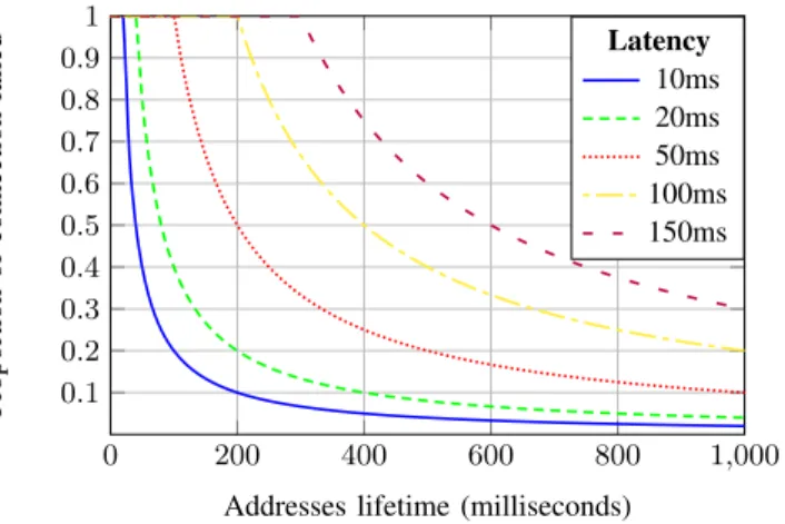
Our loss of packets is not distribute like a standard network error, each packet does not have a probability of failure, but the connection seems to be broken for a short duration, in one or two ways. 0 200 400 600 800 1 ,000 0 .1 0 .2 0.3 0.4 0 .5 0 .6 0 .7 0.8 0.9 1
Addresses lifetime (milliseconds)
Proportion of connection failed Latency 10ms 20ms 50ms 100ms 150ms
Figure 8: ICMP echo failure rate in function of latency
For example, in case of ICMP echo transmission between spreaders A and B, the total duration of one of packet echo reply/request will dropped is
latency∗ 2 + desync (10)
We plot in Figure 8 the theoretical ICMP echo request/reply transmission failure for a given latency in function of address lifetime, without any desynchronization of spreaders.
D. Temporal windows one old and next addresses
To reduce the loss of packets, it is possible to accept the old address of time t−1 in a temporal windows where both current
address t and t− 1 addresses are accepted. With a temporal
windows larger than the latency, no packets are dropped by synchronized spreaders.
In case of desynchronization smaller than the latency, we have to add this desynchronization duration to the temporal windows to accept all packets send in the communication. A spreader can not know if a packet is delayed due to the latency or due to a desynchronization problem.
If the desynchronization is larger than the latency, a spreader will receive packets to early. To solve it, we can add in the same way a temporal windows where both addresses of
t and t+ 1 are valid. If a spreader receives a lot of packets
on the t+ 1 address, it is a sign of desynchronization and it
could help to resynchronize both spreaders. We present our experimental results on temporal windows to accept old and future addresses in Section VII-D.
VII. PERFORMANCE TESTS A. Test beds
1) Implementation: Our implementation is based on a Netfilter module for Linux. It follows steps explained in Section V. The implementation supports configuration of the validity lifetime of one address as well than temporal windows for packets out of the current time sequence.
1 .8 2 2.2 2.4 2.6 2.8 3 0 .1 0 .2 0 .3 0.4 0 .5 0 .6 0 .7 0.8 0.9 1 RTT Time (milliseconds) Proportion of successful connections
Figure 9: RTT of UDP echo requests on the LAN
40 42 44 46 48 50 0 .1 0 .2 0.3 0.4 0 .5 0 .6 0 .7 0.8 0 .9 1 RTT Time (milliseconds) Proportion of successful connections
Figure 10: RTT of UDP echo requests on the 6to4 network
2) Networks tests: We have done several experimentations on several test beds, and this paper presents results from two of them. Our first test bed is the ideal one, in a LAN. The typical round-trip delay time (RTT) is around 2 milliseconds (ms), there are no loss or desequencing of packets. The Figure 9 depicts the cumulative distribution function of the RTT.
The second one is between a server in Germany using a 6to4 tunnel and a server with native IPv6 connectivity in France. The network has a poor quality: there are some natural packet loss (around 1%) and desequencing (around 0.5% on high network load). In our preliminary tests, the 6to4 tunnel uses to be less congested in the night, and we ran our tests in the night to avoid some random congestion issue. The Figure 10 depicts the cumulative distribution function of the RTT.
All devices of our networks are time synchronized on the same Network Time Protocol server. It does not provide a perfect synchronization.
B. Spreading consequences
1) Tests description: To evaluate the consequences of our spreading, we ran for each network three tests. The first one
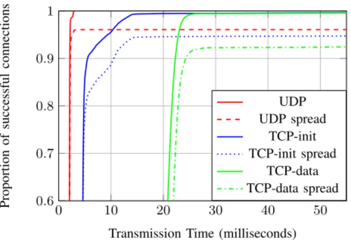
0 10 20 30 40 50 0.6 0 .7 0 .8 0 .9 1
Transmission Time (milliseconds)
Proportion of successful connections UDP UDP spread TCP-init TCP-init spread TCP-data TCP-data spread
Figure 11: Consequences of a simple spreading on the LAN
send a standard UDP echo packet, it provides a good evaluation of the network quality for the loss of packets and the latency. The second one is a simple TCP handshake initialization, without data transfer. The last one is a TCP connection with data transfer (65535 bytes). Since TCP is the most popular protocol on the Internet and that the test involves transfer of data, it is the best test to evaluate the user experience on a network with spreading. We set a timeout of 4 seconds on both TCP tests, and we consider it loss after this time.
2) Simple spreading: Since computers are not perfectly synchronized and due to the network latency, our spreading implies some loss of packets and it has consequences on the network quality. We set first a lifetime of one second for each address, without any temporal windows for old and future addresses. The Figure 11 depicts the results on the LAN and Figure 12 on the 6to4 network.
On the LAN, there are no loss of UDP packet without spreading. With spreading enabled, the percentage of failure is around 4%. UDP does not provide retransmission of data and the proportion of success does not increase with the time. The TCP handshake needs three packets to be completed, and the opening time of the majority of TCP connection is consistent with the UDP test. Some openings are delayed, and will be successfully completed with retransmission. They are not displayed on Figure 11, but we observe the same kind of results that are shown in the 6to4 network.
On the 6to4 network, loss of packets has big effect on TCP performance. For the opening of the connection, we see some steps corresponding to standard time of Linux retransmission strategy for TCP.
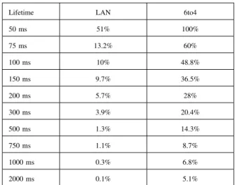
3) High frequency addresses switching, consequences on loss of packets: Of course, the lifetime of addresses has a big impact on the quality of the connection. We tried lifetime values between 50 ms and 2 seconds, and we summarize the percentage of packet loss in Table V.
We compare it to the theoretical result of Section VI-C in Figure 13. For the 6to4 network, the typical latency is around 21 ms, and we measure a desynchronization of 8 ms at the end of the experiment, it gives us around 50 ms of black hole
0 1 ,000 2,000 3,000 4,000 0.6 0 .7 0 .8 0 .9 1
Transmission Time (milliseconds)
Proportion of successful connections UDP UDP spread TCP-init TCP-init spread TCP-data TCP-data spread
Figure 12: Consequences of a simple spreading on 6to4
TABLE V: PROPORTION OF PACKET LOSS
Lifetime LAN 6to4
50 ms 51% 100% 75 ms 13.2% 60% 100 ms 10% 48.8% 150 ms 9.7% 36.5% 200 ms 5.7% 28% 300 ms 3.9% 20.4% 500 ms 1.3% 14.3% 750 ms 1.1% 8.7% 1000 ms 0.3% 6.8% 2000 ms 0.1% 5.1%
for the transmission. Our experimental result is very close to this theoretical result. But since the 6to4 network has some natural packet loss, there are more failure than excepted when the spreading effect decrease.
On the LAN, the latency is small, and the desynchro-nization is the main issue. We measure a desynchrodesynchro-nization between 0 and 30 ms, it is not stable in time of experiences. We took the middle value to plot the theoretical value with a black hole of 17 ms at each address switching.
C. Delayed packets: temporal window for the last old address
To prevent loss of delayed packets, we add a temporal window for the old address. In this temporal windows, the old and the current addresses of a sequence are accepted by the spreader. It is very efficient to decrease the loss of packets on the 6to4 network, like we can see in Figure 14.
With a temporal windows larger than the sum of the latency and the desynchronization of the network, we get the same performance than without spreading.
As depicted in Figure 15, it is not enough to prevent loss of packets on the LAN. The desynchronization is bigger than the
0 200 400 600 800 1 ,000 0 .1 0 .2 0.3 0.4 0 .5 0 .6 0 .7 0.8 0.9 1
Addresses lifetime (milliseconds)
Proportion of connection failed Real 6to4 Theory 6to4 l=50ms Real LAN Theory LAN l=17ms
Figure 13: Proportion of failed ICMP echo transmission
0 1 2 3 4 5 0.6 0.7 0.8 0.9 1
Transmission Time (seconds)
Proportion
of
successful
connections
Old address validity No spreading 0 ms 4 ms 8 ms 20 ms 40 ms
Figure 14: TCP test with transmission of data on the 6to4 network in function of temporal windows for the old address
latency and some packets come to early for a spreader. In this case, we need to accept the previous address on the spreader desynchronized in the future as well than the next address on the other spreader.
D. Desynchronization: temporal window for next address
To solve the desynchronization issue on the LAN, we add a temporal windows for the next address. During this temporal windows, both actual address and next address of the sequence are accepted by the spreader.
We plotted the results of UDP test in Figure 16, with a lifetime of 200 ms and a temporal windows for the old address of 60 ms.
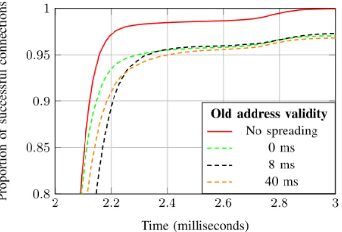
Adding a temporal windows for the next address is not enough to avoid any loose of packet. We need to accept the old address on the spreader with a clock ahead of the real time. We wrote in Table VI the loss of packets with respect of both temporal windows for the old and the future address on the LAN. Since the desynchronization is not stable in the time of the experience, some values can be confusing. The loss can decrease if we increase the temporal windows. However, if
2 2 .2 2.4 2.6 2.8 3 0.8 0 .85 0 .9 0 .95 1 Time (milliseconds) Proportion of successful connections
Old address validity No spreading
0 ms 8 ms 40 ms
Figure 15: UDP test in function of temporal windows for the old address on the LAN
2 .2 2.4 2.6 2.8 3 3.2 0.9 0 .92 0.94 0 .96 0 .98 1 RTT Time (milliseconds) Proportion of successful connections
Next address advance No spreading
0 ms 4 ms 12 ms 40 ms
Figure 16: Next address temporal windows on the LAN
both temporal windows are larger than the desynchronization, there are no more loss of packets. A value of 64 milliseconds is enough here.
VIII. CONCLUSION
The spreading of addresses is an innovative and new solution to identify a connection. This is a new mechanism to protect against spoofing attack. Our spreading protects against
TABLE VI: INFLUENCE OF NEXT AND OLD ADDRESSES ON PACKET LOSS
% loss
Next address temporal windows (ms)
0 4 8 12 20 40 64 80 Old addr ess v alidity 0 3.5 5 3.9 3.3 3.3 4.8 3 4.9 4 6 3.3 0.8 0.9 0.5 1.3 1.1 1.5 8 2.7 2.3 0.6 0.7 0.7 0.1 0 0 12 6.4 3 2 0 0 0 0 0 20 3 2.3 0.5 0 0 0 0 0
initialization of a connection from an attacker, as well than injection of packet inside a established connection.
We described a complete protocol to securely initiate connection between spreaders, with one initialization of tem-poral sequences of addresses per flow. We did a step by step description of the spreader internal functionality, and we explain the theoretical loss of packets without any temporal windows.
With the use of temporal windows for the old address, we can protect against false positive detection of packets due to the network latency. With the use of a temporal window for the next address, we protect our solution against desynchronization of devices. We can use this information to resynchronize spreaders without external source of time.
Thanks to these temporal windows, we can achieve a very high frequency of address switching. An address is valid only for several duration of the latency in the network.
In the future works, we will evaluate algorithms to generate sequence of addresses. To simplify the work of the network administrator, the auto-configuration and the exchange of the secret between the spreaders have to be considered.
REFERENCES
[1] N. Brownlee, C. Mills, and G. Ruth, “Traffic Flow Measurement: Architecture,” RFC 2722 (Informational), Internet Engineering Task Force, Oct. 1999. [Online]. Available: http://www.ietf.org/rfc/rfc2722. txt
[2] J. Postel, “Transmission Control Protocol,” RFC 793 (INTERNET STANDARD), Internet Engineering Task Force, Sep. 1981, updated by RFCs 1122, 3168, 6093, 6528. [Online]. Available: http: //www.ietf.org/rfc/rfc793.txt
[3] T. Aura, “Cryptographically Generated Addresses (CGA),” RFC 3972 (Proposed Standard), Internet Engineering Task Force, Mar. 2005, updated by RFCs 4581, 4982. [Online]. Available: http: //www.ietf.org/rfc/rfc3972.txt
[4] P. Ferguson and D. Senie, “Network Ingress Filtering: Defeating Denial of Service Attacks which employ IP Source Address Spoofing,” RFC 2827 (Best Current Practice), Internet Engineering Task Force, May 2000, updated by RFC 3704. [Online]. Available: http://www.ietf.org/rfc/rfc2827.txt
[5] T. Narten, G. Huston, and L. Roberts, “IPv6 Address Assignment to End Sites,” RFC 6177 (Best Current Practice), Internet Engineering Task Force, Mar. 2011. [Online]. Available: http://www.ietf.org/rfc/ rfc6177.txt
[6] M. Dunlop, S. Groat, W. Urbanski, R. Marchany, and J. Tront, “Mt6d: A moving target ipv6 defense,” in MILITARY COMMUNICATIONS CONFERENCE, 2011 - MILCOM 2011, Nov 2011, pp. 1321–1326. [7] M. Bagnulo, A. Garcia-Martinez, and A. Azcorra, “An architecture
for network layer privacy,” in Communications, 2007. ICC ’07. IEEE International Conference on, June 2007, pp. 1509–1514.
[8] X. Cheng, J. Bi, and X. Li, “Swing - a novel mechanism inspired by shim6 address-switch conception to limit the effectiveness of dos attacks,” in Networking, 2008. ICN 2008. Seventh International Con-ference on, April 2008, pp. 267–272.
[9] S. Amante, B. Carpenter, S. Jiang, and J. Rajahalme, “IPv6 Flow Label Specification,” RFC 6437 (Proposed Standard), Internet Engineering Task Force, Nov. 2011. [Online]. Available: http: //www.ietf.org/rfc/rfc6437.txt
[10] Q. Hu and B. Carpenter, “Survey of Proposed Use Cases for the IPv6 Flow Label,” RFC 6294 (Informational), Internet Engineering Task Force, Jun. 2011. [Online]. Available: http: //www.ietf.org/rfc/rfc6294.txt