HAL Id: hal-02484330
https://hal.archives-ouvertes.fr/hal-02484330v2
Submitted on 2 Apr 2020
HAL is a multi-disciplinary open access
archive for the deposit and dissemination of
sci-entific research documents, whether they are
pub-lished or not. The documents may come from
teaching and research institutions in France or
abroad, or from public or private research centers.
L’archive ouverte pluridisciplinaire HAL, est
destinée au dépôt et à la diffusion de documents
scientifiques de niveau recherche, publiés ou non,
émanant des établissements d’enseignement et de
recherche français ou étrangers, des laboratoires
publics ou privés.
Space-time pattern extraction in alarm logs for network
diagnosis
Achille Salaün, Anne Bouillard, Marc-Olivier Buob
To cite this version:
Achille Salaün, Anne Bouillard, Marc-Olivier Buob. Space-time pattern extraction in alarm logs for
network diagnosis. MLN 2019: 2nd IFIP International Conference on Machine Learning for
Network-ing, Dec 2019, Paris, France. pp.134-153, �10.1007/978-3-030-45778-5_10�. �hal-02484330v2�
network diagnosis
Achille Sala¨un1,2, Anne Bouillard1, and Marc-Olivier Buob1 1
Nokia Bell Labs
{achille.salaun, anne.bouillard, marc-olivier.buob}@nokia.com
2
CNRS, Samovar, T´el´ecom SudParis, Institut Polytechnique de Paris
Abstract. Increasing size and complexity of telecommunication net-works make troubleshooting and network management more and more critical. As analyzing a log is cumbersome and time consuming, experts need tools helping them to quickly pinpoint the root cause when a prob-lem arises. A structure called DIG-DAG able to store chain of alarms in a compact manner according to an input log has recently been proposed. Unfortunately, for large logs, this structure may be huge, and thus hardly readable for experts. To circumvent this problem, this paper proposes a framework allowing to query a DIG-DAG in order to extract patterns of interest, and a full methodology for end-to-end analysis of a log. Keywords: Fault diagnosis· pattern matching · online algorithm.
1
Introduction
Telecommunication networks management becomes a more and more challenging problem for operators. Indeed, on one hand, their infrastructures involve more and more devices, new technologies and possibly new manufacturers. On the other hand, network providers aim at offering a quality of service according to the Service-Level Agreements (SLAs) established with their clients. Thus, there is a strong need for fault management in order to save money, time, and human resources.
That is why network infrastructures are in general monitored. Monitoring solutions evaluate network performances through measurements. They can also collect alarms raised by the equipment involved in the infrastructure. The re-sulting file storing those messages is called a log.
Alarm logs are the raw material used by the expert to understand the cause of outages. Unfortunately, logs are in practice often very verbose and may be noisy. The large number of observed machines and alarm types in the log leads to an important volume of alarms, which complicates the extraction of relevant information, especially when multiple log files are involved. Log analysis is thus a difficult, cumbersome and time-consuming task. Network operators need tools helping them to pinpoint root causes of major incidents and understand the erroneous processes leading to major failures.
State of the art on root-cause analysis. Root cause analysis (RCA) in telecommunication networks has been extensively studied as observed in [13].
Many solutions use neural networks (NN). For instance, [14] investigates the performance of several types of NNs for fault diagnosis of a simulation heat exchanger. In particular, the authors trained a multi-layer perceptron to map symptoms onto causes. Regarding the application, it may be impossible to ob-tain enough training with ground truth. In this case, supervised learning is not possible. Therefore, the authors also trained self-organizing maps to cluster the observed symptoms. The observation space is mapped onto a 2D grid and clusters are derived a posteriori. However, the interpretation of those clusters remains dif-ficult. [17] considers several time-series and build the correlation matrix of these signals at each instant. The idea is then to train a convolutional and attention-based auto-encoder to predict sequences of correlation matrices. Correlation can be drawn between faulty signals and other ones. Unsupervised, the model takes into account temporal dependencies but is hardly interpretable.
Bayesian networks (BN) are also common in RCA. Thus, in [2], the authors split latent causes and observed symptoms into a bipartite BN. Symptoms are either described by some features or by checking some rules. If the probabilistic framework favors interpretability of the results, BNs generally face scalability issues. Indeed, increasing the complexity of the system dramatically increases the amount of memory to store conditional probabilities. [16] proposes to build BNs for root-cause analysis in an oriented-object fashion. This helps to design proper BNs with regard to prior knowledge about the system structure (thanks to the definition of BN functions), but automation of the model construction is unclear especially when prior knowledge is unavailable.
In order to explain faulty requests in the eBay Internet Service System, [6] trains a decision tree classifying faults and successes. Once trained, the path of a given faulty request is then used as a description of its root cause. The simplicity of decision trees makes them easy to interpret. Nevertheless, increasing the com-plexity of the system induces instability in the training phase [3]. Interpretability may be unclear in such a situation.
Some other solutions comes from pattern matching. [7] introduces a variation of the Smith-Wasserman algorithm [12] which evaluates the similarity between two sequences of events. Indeed, root cause may belong to alarm floods that are similar to a faulty one. [10] splits events streams into chunks that are then compared to a reference database. [15] uses Finite State Machines storing prior faulty patterns. It is possible to update the stored patterns a posteriori.
An other approach, [4], proposes an RCA tool inspired from pattern match-ing techniques. It builds online an automaton stormatch-ing space-time causalities be-tween symbols observed in a log. Its construction is unsupervised without losing in interpretability. Moreover, prior knowledge is optional though adding such knowledge makes the resulting structure lighter by discarding irrelevant causal-ities. Nonetheless, the size of the structure is usually too large for a direct use. For now, we still lack a tool to exploit such a structure and this paper is a first attempt to overcome that lack.
Contributions. Most of works described above try to find the root cause of a failure or to find correlation between alarms.
In this paper, we rather try to find chains of cascading alarms explaining why a given incident has occurred. In our approach, we process an input log with some optional prior knowledge (e.g., the network topology). This information is used to train a data structure, called DIG-DAG [4], which is designed to store every chain of alarm present in the input log.
Such a structure is usually too large to be directly interpretable by an expert. That is why we require a convenient way to extract relevant faulty patterns.
The contributions of this paper are twofold:
1. First, we propose a new query system, allowing to extract small faulty pat-terns stored in a DIG-DAG and matching the query issued by an expert. Outputs not only contain the possible root causes of a failure, but also the entire chain of alarms leading to the failure.
2. Second, we propose an end-to-end methodology for log analysis. It involves the DIG-DAG and our new query system, but also additional techniques us-ing graph reductions and clusterus-ing techniques. We demonstrate the tractabil-ity of our framework through the analysis of logs issued by real systems.
Outline of the paper. The remaining of the paper is organized as follows. Section 2 recalls the DIG-DAG construction from an input log of alarms (and eventual prior knowledge). Section 3 presents the query system built on top of DIG-DAG, which is the core of our contribution. In Section 4 details an end-to-end methodology for log analysis and hints to cope with large logs of alarms. Section 5 illustrates our proposal on real datasets. Finally, Section 6 concludes the paper.
2
From log to space-time pattern storage
In this section, we recall the necessary background related to DIG-DAG, a data structure introduced in [4] able to store space-time patterns. To fix notations, Section 2.1 formally defines our representation of an alarm log. Section 2.2 in-troduces directed interval graph (DIG), a graphical representation of the log. Finally, Section 2.3 presents the DIG-DAG.
2.1 Alarm logs
Nowadays, network operators rely on monitoring solutions to manage their in-frastructures. Such solutions centralize alarms raised by the equipment into ded-icated files called logs.
More formally, an alarm log is a finite sequence of timestamped events. More precisely, we consider that an event is a pair (σ, [s, t]), where σ is a symbol and [s, t] is a non-empty interval of R+ representing the time interval during which
e.g., the name of the corresponding alarm, its severity, the impacted machine, etc. This constitutes the space aspect of the event. We denote by Σ the set of all possible symbols and assume this set finite. For an event ` = (σ, [s, t]), we denote its symbol by λ(`).
A log is then denoted by L = ((σi, [si, ti])i∈{1,...,n}). We assume, without loss
of generality that:
– the values (si) and (ti) are all distinct. Indeed, tie-breaking rules can be used
if it is not the case;
– if σi= σjfor some distinct i and j, then [si, ti]∩[sj, tj] = ∅: the corresponding
events do not temporally overlap. If this is not the case, these two events can be replaced by (σi, [si, ti] ∪ [sj, tj]).
A log can be processed online. An event is said to be active at a time if it corresponds to a pending alarm at this time. More formally, given log L and time τ , an event (σ, [s, t]) of L is active at time τ if τ ∈ [s, t]. We note Aτ the
set of active events of log L at time τ . The observed log at time τ is defined as Lτ
def
= ((σ, [s, t]) ∈ L|s < τ ).
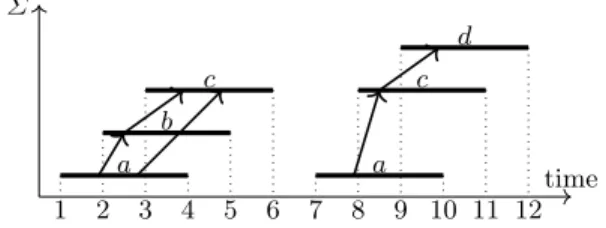
Example 1. Consider alphabet Σ = {a, b, c, d} and log L = ((a, [1, 4]), (b, [2, 5]), (c, [3, 6]), (a, [7, 10]), (c, [8, 11]), (d, [9, 12])). At time τ = 5.5, we have A5.5 =
{(c, [3, 6])} and
L5.5= ((a, [1, 4]), (b, [2, 5]), (c, [3, 6])).
2.2 DIG: a graph-based representation of an alarm log
In this paragraph, our goal is to represent the log of alarms in a more structured way. Indeed, fault management is based on finding correlation between alarms, hence exhibiting some structure in the log. To do so, we first define the notion of potential causality which enables to translate the log into a graph.
Two events share a potential causality if they are space-related and if they share a potential time causality. Two events are space-related if their symbol lies in C ∈ Σ2, which gathers all the relevant pairs of symbols. For example, C
can be tuned to consider the topology of the network (see Sec. 4). Two events share a potential time causality if one of the events occurs before the other, and if their activity period overlap. More formally, we say that event ` = (σ, [s, t]) is a potential cause of `0= (σ0, [s0, t0]) if
– σσ0∈ C: ` and `0 are space-related ;
– s0∈ [s, t]: ` and `0 are co-occurrent and ` is active before `0.
This potential causality is denoted by ` → `0.
The directed interval graph (DIG) of L with space relation C is a labeled directed graph (L, →, λ) where:
– L is the set of vertices; – → is the set of arcs;
– λ : L → Σ is the labeling function inherited form the event: each ver-tex/event is labeled with its symbol.
This directed graph is acyclic because of the time causality contained in →. As shown in Figure 1, a DIG can be disconnected.
Example 2. If C = {ab, ac, bc, cd}, then (a, [1, 4]) → (b, [2, 5]) holds, but (b, [2, 5]) 9 (a, [1, 4]) and (a, [1, 4]) 9 (c, [8, 11]) as they break the time causality, and (a, [7, 10]) 9 (d, [9, 12])) because ad /∈ C.
The DIG corresponding to the log L of Example 1 is represented on Figure 1.
a b c a c d 1 2 3 4 5 6 7 8 9 10 11 12 time Σ
Fig. 1: DIG of L defined in Example 1.
We call space-time pattern or pattern of the log any word of Σ∗any label of a path of its DIG. The denomination space-time comes after potential causalities that can be issued either from topological or from temporal reasons.
2.3 DIG-DAG: a data structure for storing space-time patterns DIG-DAG is a deterministic automaton-like structure able to store and count every space-time pattern of a log. It is the base of our root-case analysis approach. We use the formal language notations. In particular, the empty word is denoted by ε.
Definition 1 (DIG-DAG). Let L be an alarm log on alphabet Σ, with spatial relation C and A ⊆ L a set of active events.
A DIG-DAG (V, E, λ, A) of (L, →, λ) is a quadruple satisfying:
– (V, E) is a directed acyclic graph with a unique vertex q0 with in-degree 0,
called the root;
– λ is a labeling function λ : V → Σ ∪ {ε} with λ(q0) = ε and ∀u ∈
V \{q0}, λ(u) ∈ Σ;
– for each vertex u ∈ V and for each σ ∈ Σ, vertex u has at most one successor v ∈ V such that λ(v) = σ;
– each path `1, ..., `k of the DIG corresponds to a path q0, u1, ..., uk ∈ Vk+1
such that λ(`i) = λ(ui) for all i ∈ {1, . . . , k} and conversely;
– A ⊆ V is a subset such that u ∈ A if and only if for all paths from the root to u there exists a path in (L, →, λ) ending in an active vertex with the same label. In other words, for each path q0, u1, ..., u there exists a path `1, ..., `u
in (L, →, λ) such that λ(`i) = λ(ui) and `u is active.
One can notice that, given a log L and a spatial relation C, the DIG is unique but not the DIG-DAG. For example, the DIG-DAG can be minimized or not. We assume in the rest of the paper that the DIG-DAG is built according to the deterministic algorithm presented in [4]. This algorithm can be performed online by processing events in their chronological order.
One of its advantages is its capability to count and store the number of occurrences of each space-time pattern occurring in (L, →, λ). More precisely, w : E → N is a weight function counting the number of occurrences of any pattern ending with that arc: w((u, v)) = n if for any path q0, . . . , u, v, the
pattern λ(q0) · · · λ(u)λ(v) corresponds to n paths of (L, →, λ).
Finally, as already mentioned above, the DIG-DAG can be interpreted as a special case of a deterministic automaton, where q0 is the initial state and the
labels are deported to the targets of the transitions.
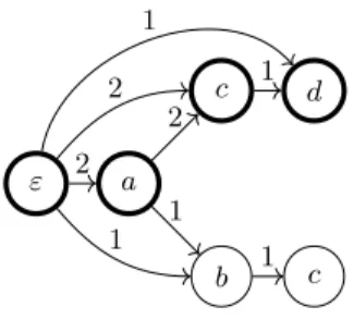
Example 3. Figure 2 shows the DIG-DAG built from DIG (L, →, λ) (cf. Exam-ple 1) at time 9.5: the last three events of the log are active. The weights are depicted above the arcs. For example, a and ac occur twice, while abc occurs only once. Active vertices are represented in bold.
ε a b c c d 2 1 2 1 1 2 1 1
Fig. 2: DIG-DAG built from log L of Example 1; bold vertices are the active states at time τ = 9.5.
To sum up, a DIG-DAG is a graph structure able to store and count any space-time pattern occurring is an alarm log. The size of this structure can grow exponentially with the size of the log. For example, root’s out-degree is exactly the size of the alphabet Σ and the depth of the structure is the size of a longest path in the corresponding DIG. The rest of the paper is devoted to the extraction of patterns of interest.
3
Pattern extraction
In this section, we present a generic solution to extract patterns of interest by queries.
This section presents a new framework able to isolate patterns matching input queries. These patterns are represented as sub-DIG-DAGs:
Definition 2 (sub-DIG-DAG). Let D = (V, E, λ, A) be a DIG-DAG. For every subgraph (V0, E0) of (V, E), the 4-tuple D0 = (V0, E0, λ|V0, A ∩ V0) is a
sub-DIG-DAG of D.
Remark that a sub-DIG-DAG is not necessarily a DIG-DAG: it may have several roots and be disconnected.
Sub-DIG-DAGs are stable with graph operations like intersection, union, difference.
Definition 3 (query and its resulting sub-DIG-DAG). A query is a 5-tuple Q = (D, S, T, Vi, Ei), where D = (V, E, λ, A) is a DIG-DAG, S, T, V0 ⊆ V
and E0⊆ E. The result of the query is the largest sub-DIG-DAG (E0, V0, λ0, A0)
of D such that: – V0⊆ Vi, E0 ⊆ Ei;
– the vertices with in-degree 0 are in S; – the vertices with out-degree 0 are in T . The result of the query is denoted by D(Q).
Intuitively, the sub-DIG-DAG of D resulting from a query Q = (D, S, T, Vi, Ei)
is the subgraph of D whose maximal paths all start in S and end in T . These paths only traverse vertices of Vi and arcs of Ei.
3.1 Regular queries
The definition of queries is very broad, and in this paragraph we restrict to queries parametrized by a finite automaton, and local properties on the vertices and arcs. Intuitively, the role of the finite automaton is to extract patterns satisfying some relations between vertices, while local properties select vertices and arcs. These properties do not only depend on the symbols of the nodes (which could otherwise have been done with an automaton), but rely on information that can be attached to the nodes. For example, this can be useful to extract nodes that have been recently active or arcs satisfying some weight-based properties.
Definition 4 (Regular query). Let M be a finite automaton, and Pv and Pe
be two properties. The regular query R(S, T, M, Pv, Pe) = (S, T, Vi, Ei), where:
– for all v ∈ Vi, v satisfies Pv;
Algorithm 1: Input query based sub-DIG-DAG extraction
Input: D, M = (Q, Σ, δ, I, F ), S, T, Pv, Pe
Output: a sub-DIG-DAG D0 // Phase 1: Forward exploration foreach u ∈ V do Q1(u) ← ∅;
foreach u ∈ V (in the topological order) do if u ∈ S ∩ Pv then Q1(u) ← Q1(u) ∪ I;
foreach v ∈ V ∩ Pv such that (u, v) ∈ E ∩ Pedo
Q1(v) ← Q1(v) ∪ {q0∈ Q | ∃q ∈ Q1(u), δ(q, q0) = λ(v)}
// Phase 2: Backward exploration and decision V0← ∅; E0← ∅;
foreach u ∈ V do Q2(u) ← ∅;
foreach u ∈ V (in the reverse of the topological order) do if u ∈ T ∩ Pvthen Q2(u) ← Q2(u) ∪ (Q1(u) ∩ F );
if Q2(u) 6= ∅ then
V0← V0∪ {u}
foreach v such that (v, u) ∈ E ∩ Pe do
if {q ∈ Q1(v) | ∃q0∈ Q2(u), δ(q, q0) = λ(v)}} 6= ∅ then
E0← E0∪ {(v, u)};
Q2(v) ← Q2(v) ∪ {q ∈ Q1(v) | ∃q0∈ Q2(u), δ(q, q0) = λ(v)}
return D0= (V0, E0, λ|E0, A ∩ V0)
– D(R(S, T, M, Pv, Pe)) contains all the paths of D(Q) labeled by a word
rec-ognized by M. Consequently, Vi and Ei are respectively defined by the set of
vertices and arcs belonging to one of those paths;
– D(R(S, T, M, Pv, Pe)) is the minimal sub-DIG-DAG satisfying those
prop-erties.
Algorithm 1 computes the sub-DIG-DAG corresponding to a regular query. We assume that we know a topological order of the vertices. For this one can either use a classical algorithm (see [8] for example), or the topological order can be computed on-the-fly at the DIG-DAG construction.
Algorithm 1 has two phases: the first one identifies, by a forward traversal of the DIG-DAG all the possible paths starting from S, having vertices and arcs satisfying Pv and Pe and whose label are prefixes of words recognized of the
automaton. For this, a set Q1(u) is attached to each node, containing all the
states of the automaton that can be reached from a vertex in S.
The second phase performs a backward traversal and identifies the vertices and arcs in the sub-DIG-DAG. For each vertex u, Q2(u) is the subset of states
in Q1(u) such that there is a path from u to T labeled similarly to a path from a
state of Q2(u) to a final state in the automaton. The vertices and arcs involved
in these paths constitute the sub-DIG-DAG.
More formally, let M = (Q, Σ, δ, I, F ) be a finite automaton where Σ denotes its alphabet, Q the its set of states, I its initial states, F its final states and δ its transition map. We use the automaton interpretation of a DIG-DAG: the label of a transition is the label of the extremity of the arc. Thus, the label of a path
in the DIG-DAG does not take into account the label of the first node of the path.
We show next that the result of Algorithm 1 is the sub-DIG-DAG corre-sponding to the regular query as defined in Definition 4.
Let us first state some properties of Q2(u).
Lemma 1. With the above notations,
– ∀u ∈ V0, p ∈ Q2(u), ∃v ∈ V0, q ∈ Q2(v) such that (u, v) ∈ E0 and λ(v) ∈
δ(p, q);
– ∀v ∈ V0, q ∈ Q2(u), ∃u ∈ V0, p ∈ Q2(v) such that (u, v) ∈ E0 and λ(v) ∈
δ(p, q);
– for all v ∈ V0, for all q ∈ Q2(v), there exists a path from a vertex s ∈ S to
v corresponding to a path from i ∈ I to q in M; – for all v ∈ V0, for all q ∈ Q
2(v), there exists a path from v to a vertex t ∈ T
corresponding to a path from q to f ∈ F in M.
Proof. The first two statements are deduced from lines 5 and 12 of the algorithm, that is the construction of Q1 and Q2. The last two statements are obtained by
induction from the two firsts.
We prove that the resulting sub-DIG-DAG is indeed the smallest one containing the intersection of D and M.
Theorem 1. Consider the regular query R(S, T, M, Pv, Pe), and let D0 be the
sub-DIG-DAG returned by Algorithm 1. We have D0= D(R(S, T, M, Pv, Pe)).
Proof. We have to check the four properties of Definition 4. The two firsts are straightforward, as all vertices and arcs added to V0 and E0 respectively check Pv and Pv (lines 9-13).
We now check the third property: let p = u1, . . . , ufbe a path in D labeled by
a word accepted by M, with u1∈ S and uf ∈ T . Let q1, . . . , qf be a sequence of
states visited by M for accepting this word. For all i, by construction, qi∈ Q1(ui)
(line 5). As qf ∈ F and uf ∈ T , qf ∈ Q2(uf) (line 9), and then, qi∈ Q2(ui) for
all i (line 14): all the arcs of the path are kept.
Finally, we have to check the minimality of the structure, that is that all the arcs of the graph returned by the algorithm belong to a path labeled by a word recognized by M. This is a consequence of Lemma 1: consider an arc (u, v). One can build a path s ∈ S u → v t ∈ T corresponding to qi ∈ I ∩ Q2(s) p ∈ Q2(u) → q ∈ Q2(v) qf ∈ F ∩ Q2(t) by applying items
3, 1, 4 of the Lemma 1.
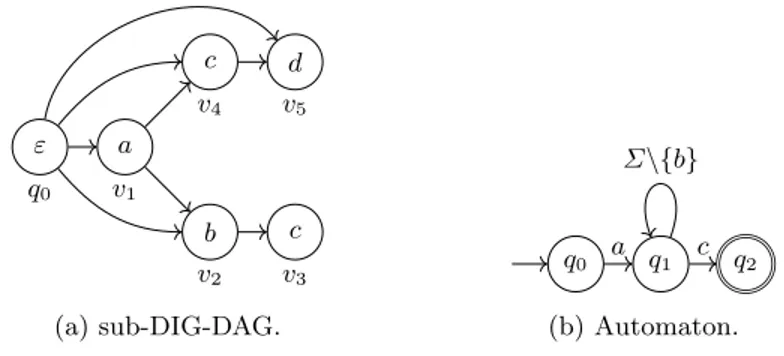
Example 4. Let us extract the patterns satisfying the regular expression a(Σ \ {b})∗c from the DIG-DAG represented in Figure 3a, that is all the paths starting
by a, ending c and not containing any b. We choose S = {q0}, T = V . Nodes of
the DIG-DAG are numbered according a topological order. The regular expres-sion is represented by the automaton shown in Figure 3b. The sub-DIG-DAG extraction steps of Algorithm 1 are depicted on Figure 4. Phase 1 is displayed
from 4a to 4e and phase 2 from 4f to 4j. Sets Q1(.) are reported below each
vertex for phase 1, and Q2(.) are for phase 2. Arcs and vertices that are added
to E0 and V0 are represented in bold, and those non selected are dashed.
ε q0 a v1 b v2 c v3 c v4 d v5 (a) sub-DIG-DAG. q0 a q1 c q2 Σ\{b} (b) Automaton.
Fig. 3: DIG-DAG and automaton used for Algorithm 1 in Example 4.
3.2 Sub-DIG-DAG simplification
Queries and in particular regular queries allow to select patterns of interest. Ideally, the extracted sub-DIG-DAG should be easily readable. As we will see in Section 5, the number of vertices is often limited, but it happens that the average degree of the sub-DIG-DAG is too high to get a readable graphical representation. In this paragraph, we present three methods to improve and simplify the graph. Note that this simplification cannot be considered as sub-DIG-DAG extraction, as they might change the structure, by merging nodes, erase paths and are not compatible with weights. This is not a big issue since these operations are just for graphical representations.
Transitive reduction. The aim of the transitive reduction is to decrease the number of arcs. Introduced in [1], this operation removes every arc e = (u, v) whenever there exists another path between nodes u and v. The resulting graph is the minimal subgraph (for the arc-inclusion order) that does not break the connectivity of each connected component of the graph. The transitive reduction removes some paths from the sub-DIG-DAG, but keeps the longest ones.
Minimization. As said above, a DIG-DAG can be seen as a deterministic automaton. Moreover, it is acyclic. As a sub-DIG-DAG is a subgraph of the DIG-DAG, it can also be seen as a deterministic automaton if it has a single source node. Still, we can use Revuz algorithm [11] to minimize it. Dedicated to
ε {q0} a ∅ b ∅ c ∅ c ∅ d ∅
(a) Phase 1; Initialization ε {q0} a {q1} b ∅ c ∅ c ∅ d ∅ (b) Ph. 1; vertex q0 ε {q0} a {q1} b ∅ c ∅ c {q1, q2} d ∅ (c) Ph. 1; vertex v1 ε {q0} a {q1} b ∅ c ∅ c {q1, q2} d ∅ (d) Ph. 1; vertex v2 ε {q0} a {q1} b ∅ c ∅ c {q1, q2} d {q1} (e) Ph. 1; vertex v4 ε ∅ a ∅ b ∅ c ∅ c ∅ d ∅ (f) Phase 2; Initialization ε ∅ a ∅ b ∅ c ∅ c ∅ d ∅ (g) Ph. 2; vertex v5 ε ∅ a {q1} b ∅ c ∅ c {q2} d ∅ (h) Ph. 2; vertex v4 ε ∅ a {q1} b ∅ c ∅ c {q2} d ∅
(i) Ph. 2; vertices v3and v2
ε {q0} a {q1} b ∅ c ∅ c {q2} d ∅ (j) Ph. 2; vertex v1 and D0
acyclic deterministic automaton, this algorithm merges equivalent states from the leaves to the root. The resulting sub-DIG-DAG is minimal and recognizes exactly the same patterns. However, some states (resp. arcs) having different weights may be merged in the process.
Source simplification As said at the end of Section 2, the size of the DIG-DAG grows exponentially with the size of the log. This means that there can be numerous vertices with the same label, especially corresponding to the same occurrence of an event. When querying a DIG-DAG, the set S might be described by some property (a given symbol, and set of symbols), and many sources might have the same label. We observe that many of them can have the same sets of successors. Source simplification parses the source nodes and merges those with the same set of successors. Here again, this operation might not be compliant with the arc weights.
4
End-to-end analysis of an alarm log
In this section, we explain how to apply the approach described in Sections 2 and 3 for the end-to-end analysis of an alarm log in a root-cause analysis context. We assume that the log is given and there is no constraint for performing it online (even if some steps can be performed online). In Section 4.1, we explain the general approach, and in Section 4.2, we give some solutions when the log is too large for the analysis to be scalable.
4.1 General approach of the analysis
Log parsing. The first step is to transform the raw log into a sequence of events. This includes fixing the alphabet, fixing the activity period of each event, and the time τ when the construction of the log stops.
Alphabet of the log: The choice of the alphabet is decided based on the features one wants to take into account during the analysis. The most relevant features are:
– the name of the alarm: this is generally a short text or a number;
– the emitting machine, represented by its identifier. This can be a machine, the port of a switch, a cell in a wireless network, etc.;
– the severity of the alarm, represented by a number or a color, that grows or becomes darker with the severity.
Activity period of an event: Depending on whether the log has already been pre-processed or not, whether an alarm has a cancel time or not, the activity period of an event must be carefully defined.
The simple case is when an alarm has a emission time and a cancel time, as they respectively define the star time and the end time of the activity period.
When only the emission time is available, this defines only the start time of the activity period. Its end has to be defined.
In some alarm logs, emission times occur at precise dates. This is the case for example for KPIs, when their emission is set a few times per hour. In this case and in order to ensure time causality, a good choice would be to set an activity period a little longer than the periodicity of the measurements.
If there is no such periodicity, then the time interval can be set up by studying the average rate of the events. More details on the choice of the activity period can be found in [4].
Fixing time τ : Even if a log is given as a file and the analysis can be performed for the whole log, it might be a better idea, sometimes, to stop the construction before. For example, a peak of alarms detected at time τ indicates that a major failure is arising in the network at that time. The origin of the problem occurs before that peak. Moreover, queries of the DIG-DAG can make advantage the active alarms at time τ .
DIG-DAG construction. Once the log has been well defined, the potential space causality C is required to build the DIG-DAG. We give below some exam-ples:
– if no information is available, then C is simply Σ2;
– it the geographic location of the network equipment is known (antennas and cells in a wireless network for example), then σσ0 ∈ C if and only if the symbols σ and σ0 represent machines are distant of no more than a few kilometers.
– if some logical behavior is known, such as a certain type of element or ap-plication only communication with some other types of machines, one can build C based on these possible communications.
The DIG-DAG can then be built. Note that additional information can be added to the structure, such as the weight of the arcs, defined in Section 2.3, or the last date of activation of each vertex, mentioned in Section 3.
Query of the DIG-DAG. Once the DIG-DAG is built, it stores every space-time pattern of the log and one can query it. For a regular query, parameters are S, T, M, Pv, Pe(see Section 3.1). Let us give some examples.
Filtering the arcs: this is done by defining property Pe. Assume that one wants
to extract parts of the DIG-DAG such that there are strong correlations between the nodes. This is done by using the weights of the arcs, and more precisely, the ratio r defined in [4], such that for each arc (u, v) of the DIG-DAG, r((u, v)) = w((u, v))/|L|v, where |L|v is the number of occurrences of v in log L. This is
the ratio between the number of time patterns ending by arc (u, v) has been observed in the log and the total number of occurrences of v in the log. If this ratio approaches 1, this means that v is strongly and positively correlated to
these patterns. Property Pewill then select the arcs having a ratio above a given
threshold ρ.
Filtering the nodes: this is done by defining property Pv. Assume that one might
want to discard alarms having the lowest severity to focus on the more important messages. This is then equivalent to select a subset of Σ. Assume that one wants to focus on recent alarms only. Then Pv can be set to select nodes that have
been recently active.
Sources: We now define S, the possible sources of the paths. By default, one can choose S = {q0} to keep every patterns. On the contrary, one could decide to
focus on some types of alarms.
Targets: For the definition of T , one may want to focus on critical events. A good choice, especially if τ has been chosen in a peak of alarm, is to focus on active alarms active at τ that have a high severity level.
More specific queries: for more specific queries, the automaton M can be defined. This can for example be used to follow and check the propagation of faults. For example, to check the propagation of a faulty behavior from a machine m1 to
another machine m2, one may define an automaton accepting words of the form
Σ1∗Σ2∗, where Σi is the set of alarms emitted from machine mi.
Once the query has been defined, the DIG-DAG is queried according to Algorithm 1. The readability of resulting sub-DIG-DAGs can be improved by using the techniques described in Section 3.2.
4.2 Dealing with huge logs
It happens that logs are too huge so that the DIG-DAG can be built in a reason-able time (or online). In this paragraph, we propose several solutions to overcome this difficulty. The first one is based on selecting relevant parts of the log, and the other ones rather modify the alphabet Σ to simplify the log.
Truncation of the log. A first solution consists in selecting only the most interesting parts of the log. Intuitively, a problem can be detected when the behavior of the alarms emission process deviates from its normal behavior. For this, we are interested in the rate on arrival of the alarms, or of a subset of alarms. Detecting the deviation as soon as possible can help targeting the root cause.
Several techniques have been proposed to detect automatically deviating be-haviors. They are all based on tracking the average arrival rate of messages: one can cite the Moving-average model [9] or [5]. In the solution proposed in the next section, we consider the latter solution, as it has been demonstrated to track de-viations more precisely. The arrival rate of messages can be computed online. Detecting sudden deviations can then be done using Tchebychev inequality.
Simplification of the alphabet. The size of the alphabet has a strong impact on the size of the DIG-DAG. Indeed, the out-degree of each vertex is bounded by the size of the alphabet.
Spamming alarms. The easiest way to simplify a log is to remove some entries. Spamming alarms are frequent alarms that do not provide information: they appear in every log, regularly, whatever the state of the machine. Removing them would not impact the retrieval of cascades of events for root-cause analysis. They can also improve the analysis by discarding irrelevant causalities. Those alarms can be learned through the observation of previous logs, or by pre-processing the log under analysis.
Clustering occurrent alarms. Another way to simplify the log is to cluster co-occurrent symbols and merge the corresponding events of the log. More precisely, we define a distance between two symbols σ and σ0 as the Jaccard distance of their emission intervals: let Iσ = ∪{`∈L | λ(`)=σ}[s`, t`] be the union of all the
intervals of time where symbol σ is emitted. The Jaccard distance of σ and σ0 is
d(σ, σ0) = 1 −|Iσ∩ Iσ0| |Iσ∪ Iσ0|
,
where | · | is the L1 norm.
This distance can be generalized to the distance between clusters the follow-ing way: let C and C0 be two sets of symbols. Let IC = ∪{`∈L | λ(`)∈σ}[s`, t`].
The Jaccard distance between C and C0 is
d(C, C0) = 1 − |IC∩ IC0| |IC∪ IC0|
.
From this distance one can build a clustering of alarms in a bottom-up ap-proach:
– fix a threshold α to merge clusters that have distance less than α;
– while the smallest distance between two any clusters is less than α, merge the two nearest clusters.
When clusters have been computed, the log needs to be simplified. The new set of symbols is the set of clusters obtained, and we replace each event (σ, [s, t]) by (C, [s, t]) is σ ∈ C, and merge all the co-occurring events having the same cluster.
As in the previous paragraph, this can be done by pre-processing the log under analysis, but could also be learned from previous logs, and the merging of events be done on-the-fly.
Projection the alphabet and two-step analysis. A third solution to limit the size of the alphabet, is to project the alphabet. For example, if the alphabet were initially based on both the emitting machine and the name of the alarm, one can build a DIG-DAG by projecting the alphabet on the machines only or the alarm
names only. By doing this, events will have to be merged as in the paragraph above. Such a simplification of the log implies some loss of information, but projecting on the machines can help locating the problem, and projecting on the alarm name can help detecting the type of problem that occurred.
This partial information can be used for selecting a sub-set of events of the original log, and perform a second construction of a DIG-DAG: let us assume for example that we used only the information of the machines to build the first DIG-DAG, and performed a query that isolated some parts of the log, hence some machines of interest. Now, consider the original log and keep only the events emitted by the machine of interest. The size of this sub-log and of the alphabet is reduced, so the analysis can be performed by building the DIG-DAG of the sub-log and querying it.
5
Experimental results
In this section, we apply our methodology (see Section 4) to three real datasets using a computer with an Intel i7 microprocessor and 8GB RAM.
5.1 Datasets
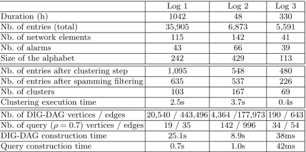
Log 1 Log 2 Log 3 Duration (h) 1042 48 330 Nb. of entries (total) 35,905 6,873 5,591 Nb. of network elements 115 142 41
Nb. of alarms 43 66 39
Size of the alphabet 242 429 113 Nb. of entries after clustering step 1,095 548 480 Nb. of entries after spamming filtering 635 537 226 Nb. of clusters 103 167 69 Clustering execution time 2.5s 3.7s 0.4s Nb. of DIG-DAG vertices / edges 20,540 / 443,496 4,364 /177,973 190 / 643 Nb. of query (ρ = 0.7) vertices / edges 19 / 35 142 / 996 34 / 54 DIG-DAG construction time 25.1s 8.9s 38ms Query construction time 0.7s 1.0s 42ms
Table 1: Experiments summary. First block describes the dimensions of the raw datasets. Second block shows the dimensions of the logs after alphabet simpli-fication. Third block highlights the gains obtained by our query system. When relevant, computation times are mentioned.
We use three private logs issued by three different GSM network elements. Each line describes a specific event which contains the alarm identifier, the ma-chine name, the emission time of the alarm, and its severity. Note that each row
describes a punctual event, i.e. the activity of the event is only characterized by its emission time. Severity is a score indicating the importance of the alarm, equal to 0 for informative messages, 1 for warnings, 2 for mid severe alarms and 3 for major failures. Each triple (machine, alarm-id, severity) corresponds to a symbol as introduced in Section 2.1.
First block of Table 1 gives for each log its size and its corresponding alpha-bet. Networks topologies are unknown.
5.2 Simplification of the alphabet and DIG-DAG construction
First of all, a potential causality relationship is defined with regard to punctual events. As logs may last several days, we consider that an event could cause another event if it occurred at most one hour earlier. This is enough to catch relevant causalities.
To limit the size of the DIG-DAG, we cluster co-occurring alarms as described in Section 4 with α = 0.3. Furthermore, we discard spamming clusters, that is clusters whose total activity period is more than 24 hours.
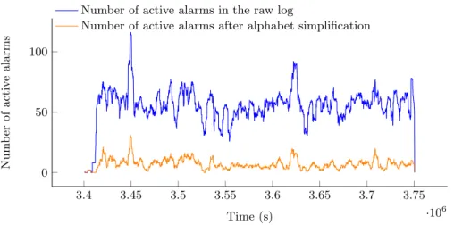
The activity in Log 1, before and after alphabet simplification, is represented in Figure 5. One can check that such simplifications did not alter the behavior observed in the original log.
3.4 3.45 3.5 3.55 3.6 3.65 3.7 3.75 ·106 0 50 100 Time (s) Num b er of activ e alarms
Number of active alarms in the raw log
Number of active alarms after alphabet simplification
Fig. 5: Number of active alarms over time (raw and simplified logs) in Log 1.
Log sizes after simplifications are shown in the second block of Table 1. Note that skipping the alphabet simplification in the RCA process leads to larger structures. For instance, Log 1 is too big to be built quick.
5.3 DIG-DAG queries
Despite their quick computation, the DIG-DAGs are hardly human-readable (see third block of Table 1). We now extract patterns leading to critical failures.
For each dataset, we query the DIG-DAG with the following parameters: – S is restricted to relevant vertices that correspond to clusters containing at
least one event of severity greater or equal to 1;
– T is restricted to critical vertices that correspond to clusters containing at least one event of severity 2 or 3;
– Pv is defined to only consider relevant vertices;
– Pe is defined to only consider arcs of ratio greater than ρ ∈ [0, 1];
– M accepts any pattern.
As we have neither prior knowledge nor expertise about the logs we studied, the described patterns are very generic. We will see however in the two next sections that these naive queries still dramatically improve DIG-DAG readability and contain relevant information about failures.
5.4 Results
Evaluating filtering of queries. This section presents results for different values of ρ. The greater this parameter, the stricter the filtering.
0 0.2 0.4 0.6 0.8 1 0 50 100 Threshold (ρ) Num b er of v ertice s (| Vρ |) 0 2 4 6 ·10−3 F raction of v ertices |Vρ |/ |V | 0 0.2 0.4 0.6 0.8 1 0 200 400 600 Threshold (ρ) Num b er of edges (| Eρ |) 0 0.5 1 ·10−3 F raction of e dges |E ρ |/ |E |
Fig. 6: Number of vertices |Vρ| (resp. edges |Eρ|) of queries in Log 1 regarding
threshold ρ (left axis). This number is divided by the number of vertices |V | (resp. edges |E|) in the whole DIG-DAG (right axis).
In Figure 6, for any ρ, queries select a small fraction of the DIG-DAG built from Log 1. This highlights the efficiency of the queries to extract patterns from the DIG-DAG. For ρ ≥ 0.7, the corresponding sub-DIG-DAG has less than 19 vertices and 35 arcs, and hence becomes small enough to be human-readable. The choice of ρ is a compromise between readability and quantity of information.
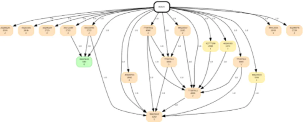
Accuracy of the queries. For each dataset, the root cause has been provided by experts. These root causes have been highlighted by experts independently of our work. When ρ = 0.7, the resulting sub-DIG-DAGs contains all the provided root causes. Moreover, the sub-DIG-DAG provides richer information than just a root cause. For example, Figure 7 depicts the sub-DIG-DAG obtained for Log 1 and contains the root cause (77397912,4004,2) provided by experts. Unfortunately, we did not get further expert feedback regarding the quality of the sub-DIG-DAGs.
Fig. 7: Sub-DIG-DAG issued by the query of Log 1 (ρ = 0.7). Labels (machine, alarm-id, severity) are indicated for each vertex. Colors depend on the sever-ity of the cluster representative. Ratios are indicated on edges.
6
Conclusion
In this article, we proposed a system of queries to extract meaningful and syn-thetic explanations from causal graph structures. The tool provided is flexible enough to allow experts to search for specific behaviors within the log. We also demonstrated how to use this tool for an end-to-end analysis.
However, human expertise is still a necessary component in the RCA process, and our goal is oriented towards self-diagnosing and self-repairing networks.
Therefore, our future works aim at automatizing the exploitation of the DIG-DAG structure. Additionally, being able to combine knowledge learnt from sim-ilar networks would help us to design a fully automatic RCA solution.
References
1. Aho, A.V., Garey, M.R., Ullman, J.D.: The transitive reduction of a directed graph. SIAM Journal on Computing 1(2), 131–137 (1972)
2. Alaeddini, A., Dogan, I.: Using bayesian networks for root cause analysis in statis-tical process control. Expert Systems with Applications 38(9), 11230–11243 (2011) 3. Aluja-Banet, T., Nafria, E.: Stability and scalability in decision trees.
Computa-tional Statistics 18(3), 505–520 (2003)
4. Bouillard, A., Buob, M.O., Raynal, M., Sala¨un, A.: Log analysis via space-time pattern matching. In: 2018 14th International Conference on Network and Service Management (CNSM). pp. 303–307. IEEE (2018)
5. Bouillard, A., Junier, A., Ronot, B.: Hidden anomaly detection in telecommunica-tion networks. In: 2012 8th internatelecommunica-tional conference on network and service man-agement (cnsm) and 2012 workshop on systems virtualiztion manman-agement (svm). pp. 82–90. IEEE (2012)
6. Chen, M., Zheng, A.X., Lloyd, J., Jordan, M.I., Brinewer, E.: Failure diagnosis using decision trees. In: International Conference on Autonomic Computing, 2004. Proceedings. pp. 36–43. IEEE (2004)
7. Cheng, Y., Izadi, I., Chen, T.: Pattern matching of alarm flood sequences by a mod-ified smith–waterman algorithm. chemical engineering research and design 91(6), 1085–1094 (2013)
8. Cormen, T.H., Leiserson, C.E., Rivest, R.L., Stein, C.: Introduction to Algorithms, 3rd Edition. MIT Press (2009)
9. Enders, W.: Stationary Time-Series Models. New York: Wiley (2004)
10. Johannesmeyer, M.C., Singhal, A., Seborg, D.E.: Pattern matching in historical data. AIChE journal 48(9), 2022–2038 (2002)
11. Revuz, D.: Minimisation of acyclic deterministic automata in linear time. Theo-retical Computer Science 92(1), 181–189 (1992)
12. Smith, T.F., Waterman, M.S., et al.: Identification of common molecular subse-quences. Journal of molecular biology 147(1), 195–197 (1981)
13. Sol´e, M., Munt´es-Mulero, V., Rana, A.I., Estrada, G.: Survey on models and tech-niques for root-cause analysis. arXiv preprint arXiv:1701.08546 (2017)
14. Sorsa, T., Koivo, H.N.: Application of artificial neural networks in process fault diagnosis. Automatica 29(4), 843–849 (1993)
15. Van Lunteren, J.: High-performance pattern-matching for intrusion detection. In: Proceedings IEEE INFOCOM 2006. 25TH IEEE International Conference on Com-puter Communications. pp. 1–13. Citeseer (2006)
16. Weidl, G., Madsen, A.L., Israelson, S.: Applications of object-oriented bayesian networks for condition monitoring, root cause analysis and decision support on operation of complex continuous processes. Computers & chemical engineering 29(9), 1996–2009 (2005)
17. Zhang, C., Song, D., Chen, Y., Feng, X., Lumezanu, C., Cheng, W., Ni, J., Zong, B., Chen, H., Chawla, N.V.: A deep neural network for unsupervised anomaly detection and diagnosis in multivariate time series data. In: Proceedings of the AAAI Conference on Artificial Intelligence. vol. 33, pp. 1409–1416 (2019)