Dynamics of rigid bodies systems with unilateral or frictional constraints

HAL Id: hal-00112294

https://hal.archives-ouvertes.fr/hal-00112294

Submitted on 31 Oct 2018

HAL is a multi-disciplinary open access archive for the deposit and dissemination of sci-entific research documents, whether they are pub-lished or not. The documents may come from teaching and research institutions in France or abroad, or from public or private research centers.

L’archive ouverte pluridisciplinaire HAL, est destinée au dépôt et à la diffusion de documents scientifiques de niveau recherche, publiés ou non, émanant des établissements d’enseignement et de recherche français ou étrangers, des laboratoires publics ou privés.

Dynamics of rigid bodies systems with unilateral or

frictional constraints

Patrick Ballard

To cite this version:

Patrick Ballard. Dynamics of rigid bodies systems with unilateral or frictional constraints: Formula-tion And Well-Posedness. David Gao; Ray Ogden. Advances in Mechanics and Mathematics, Springer, pp.3-87, 2002, �10.1007/978-1-4757-4435-4_1�. �hal-00112294�

DYNAMICS OF RIGID BODIES SYSTEMS WITH UNILATERAL OR FRICTIONAL CONSTRAINTS Formulation And Well-Posedness

Patrick Ballard

Laboratoire de Mecanique des Solides, Ecole Polytechnique, 91128 Palaiseau Cedex, France

ballard@ lms.polytechnique.fr

Abstract The classical theory of rigid bodies systems dynamics is extended into two di­ rections. First, systematic formulation of the dynamics of systems undergoing perfect unilateral constraints is derived. The general admissible form of the im­ pact constitutive equation is obtained. Well-posedness of the evolution problem is proved under the assumption that the data are analytic. Second, systematic formulation of systems undergoing frictional bilateral constraints is discussed. Well-posedness of the associated evolution problem is also demonstrated.

Keywords: Analytical Dynamics, Non-smooth Mechanics, Impact, Friction

Introduction

The point of departure of any mechanical theory is a geometric description of the system under study and all its possible (or, more exactly, admissible) evolutions. This is always a schematization. Linear forms on the space of admissible (virtual) velocities define on turn the most general representation of internal and external forces which is consistent with the geometric description. Naturally, obtaining their precise expression for a given system remains a part of the modelling process. The mass distribution leads to the definition of the kinetic energy of the system which is a positive definite quadratic form on the space of velocities. Taking a time derivative, we obtain the expression of the virtual power of inertia forces (or acceleration) in any virtual velocity. The Fundamental Principle of Classical Mechanics asserts that the virtual power of inertia forces should equal the virtual power of external and internal forces

in any admissible virtual velocity. As a consequence, we derive the equation of motion. For some class of geometric descriptions, the equation of motion, associated with some initial conditions, determines completely the subsequent motion of the system. We shall say that the evolution problem associated with the dynamics is well-posed. On the opposite, there are many examples of mechanical theories in which initial conditions and equation of motion are not enough to determine the subsequent motion of the system. This is generally attributed to the excess of schematization of the geometric description. The missing physical information is added through a constitutive law. Actually, well-posedness of the resulting evolution problem serves generally implicitly as a guideline to identify the general form of the constitutive law, although some thermodynamical considerations can also play an important part.

In this paper, we are concerned with the dynamics of rigid bodies systems. Speaking of rigid bodies systems is, actually, the geometric description of the system. It could be said that this is the most simple geometric description of solids. Working in the framework of rigid bodies system means that we are not interested in the prediction of the deformation of the bodies. It does not mean that we do not consider physical situations in which bodies deformability play a role. Let us illustrate this by examining the impact of two billiard balls. Billiard balls are always deformable. But, generally we are not interested in the deformations of the balls but only on their 'global' motion. Thus, we shall use a geometric description based on the rigidity assumption. However, we know that impacts are governed by deformation wave propagation in each of the balls. So, we can not expect the simple theory based on the geometric assumption of rigidity to be able to predict the outcome of an impact experiment. We must expect that some indetermination will remain. To get well-posedness of the theory (this is necessary to make predictions which is the final aim of any me­ chanical theory), we are led to add to the theory an impact constitutive equation. This is nothing but injecting back in the theory the outcome of the impact, since the physical phenomena which governs the impact have been eliminated. Of course, in practical situations, we have to identify the impact constitutive equa­ tion. The choices are, either to make experiments or to use a refined theory (the elasticity theory which is based on a refined geometric assumption) in order to g_et the outcome of each situation of impacts. In some situations, identifying the impact constitutive equation can represent a huge amount of work. In such a case, depending on the desired precision of the predictions of the theory, one may be led to question the relevance of the simple geometric assumption that has been adopted. The use of one geometric description or another to model a given real situation is always a compromise between the desired precision of the predictions, the amount of computation which is possible and the physical informations on the system which are available.

Since in this case, no constitutive law has to be identified, the main field of application of rigid bodies dynamics has been for a long time, celestial mechan­ ics where remarkable precision of the predictions was reached. Recently, some new fields of application of rigid bodies dynamics have emerged: robotics, granular dynamics, virtual reality, . . . All these fields have in common that de­ termining the deformation in the bodies is of no interest. Nevertheless, in these applications, impacts are possible events that have to be incorporated in the theory. Very often, precision of the predictions is not so important and one may accept very approximate impact constitutive equations. Hence, the need has emerged to enrich the well-established theory of rigid bodies dynamics with the modelling of more complicated phenomena like impacts or friction, some of them relying physically on the deformation of the bodies. This new field is often called, after Jean Jacques Moreau, Non-smooth mechanics.

Actually, those more complicated phenomena are taken into account through constraints. A constraint is a kinematical specification of the motion with which some forces are associated: the reaction forces. In general, the kinematical specification in itself is not enough to determine the reaction force: a constitutive law of the constraint has to be added. It conveys some physical assumption on the way the constraint acts.

At the time being, it seems that only the rigid bodies dynamics with perfect holonomic bilateral constraints has firm mathematical foundations in the sense that the theory ensures the well-posedness of the evolution problem describing the dynamics. In this paper, we are concerned by the systematic formulation and well-posedness of the evolution problem describing the dynamics of sys­ tems involving more general constraints such as unilateral or frictional ones. As seen above, this program will necessarily involve the discussion of some constitutive law. Our aim will not be to try to identify any realistic one but just to characterize the general forms of constitutive laws that are compatible with the well-posedness of the theory. My opinion is that well-posedness should be considered as a requirement of any theory in classical dynamics. With this idea in mind, the discussion of well-posedness is intimately connected with the discussion of constitutive laws. Actually, we shall consider well-posedness as the final aim of the theory. After having written the Fundamental Principle of Classical Dynamics, we shall look for the supplementary hypotheses that are necessary to get well-posedness. Each time an hypothesis will be made, we shall try to motivate it by a counter-example. These hypotheses will be classified into two categories. Those which convey physical assumption will be called 'constitutive' hypotheses and the other one whose aim is to prevent from mathematical pathologies will be called 'regularity' hypotheses. Since one aim is to obtain general forms of constitutive laws, one has to make sure that the constitutive laws do not depend on any particular parametrization of the system. For this reason, we are going to try to obtain intrinsic formulations of

dynamics, that is, formulations which do not rely on a particular choice for the parametrization of the system. This necessarily requires the use of the language of differential geometry. But, only the most elementary level of differential ge­ ometry is required.

The major enhancement of mathematical consistency which seems to be de­ sired at the time being concerns the modelling of impacts and that of friction. These two subjects are the major concerns in this paper and I believe that a mathematically satisfactory theory is obtained on both points-of-view of gen­ eral formulation as well as well-posedness. However, the task is far from being achieved. In this paper, we examine the cases of impacts and friction sepa­ rately. There remains to mix the two theories to discuss, for example, frictional unilateral constraints, which is not done here. The result would be a general theory of the evolution of mechanisms consisting of rigid bodies.

Section 1 recalls briefly the basics of intrinsic formulation and well-posedness of the dynamics of rigid bodies systems. The aim of this section is to provide precise description of the framework and notations. Section 2 contains also only well-known material. It shows that superimposing perfect holonomic bi­ lateral constraints does not modify the structure of the theory. In Section 3, perfect unilateral constraints are discussed. The general form for the impact constitutive equation is provided and the general formulation for the evolution problem is derived. Well-posedness is fully discussed. In Section 4, the case of general perfect non-holonomic bilateral constraints is examined. Actually, this type of constraint is a particular case of non-firm constraints which are the concern of Section 5. A complete theory of non-firm constraints is derived, including systematic formulation and well-posedness. In Section 6, the formal­ ism of non-firm constraints is applied to the description of frictional bilateral constraints. The underlying idea is that friction should be considered as a dis­ sipation mechanism obeying the Principle of Maximal Dissipation. In some cases (for example, systems of punctual particles), we recover standard dry friction laws such as Coulomb friction and, in some cases, we do not. Section 7 provides a brief description of the situations that are not contained in the above theories and the extensions of the content of the paper that could be done later on.

1. The dynamics of rigid bodies systems

1.1 The geometric assumption: rigidity

Classical mechanics postulates the existence of a three-dimensional oriented affine Euclidean space£, sometimes called the (Galilean) real world, and an absolute chronology represented (after the choice of an origin) by a real number, generally denoted by

t.

The vector space associated with £ will be denoted by E.

A solid is represented by its real world reference configuration which is nothing but a possible geometric locus of all the material points of the solid in £. The geometric assumption of rigidity can be stated as follows: the only real world configuration of that solid which can be observed are obtained from the real world reference configuration by direct isometries. Therefore, once the real world reference configuration has been fixed, any real world conguration of the solid is represented by a direct isometry q. Considering a material point of the solid identified by its location M E £ in the real world reference configuration, the current location of that material point in the configuration defined by q is:

m( M, q)

=

q(M) . ( 1.1)

Since any direct isometry on £ can be split into a translation and a rotation, the set of all direct isometries can be identified toE x §00 (where §03 denotes the set of all direct orthogonal endomorphisms on E, endowed with its standard manifold structure). It is said that E x §00 is the (abstract) configuration manifold of the rigid solid. Since its dimension is 6, we say that the rigid solid has 6 degrees of freedom (dot). Any (local) chart on the configuration manifold is called a (local) parametrization. The configuration manifold is generally denoted by Q and a configuration (an element of the configuration manifold), by q. A local chart (parametrization) will be denoted generally by '1/J. Thus, for a rigid solid, the symbol '1/J(q) denotes an element of JR6.

Other idealizations of rigid solids can appear: the infinitely thin rigid bar

whose configuration manifold is Ex §2 (§2 denotes the two-dimensional sphere equipped with its standard manifold structure) and the punctual particle whose configuration manifold is simply E.

A motion of a rigid solid is a curve on its configuration manifold (a mapping from a time interval

I

into Q). The derivative of the motion at instant

t

is denoted by q(t). It is called the (abstract or sometimes, generalized) velocity. It is an element of the tangent bundle TQ of the configuration manifold. One often encounters the name 'state space' for TQ, in which case q(t) is also called a state of the system. Since the mapping m defined by formula ( 1 . 1 ) is obviously smooth, the material velocities are expressed in terms of the (abstract) velocity by:

m = oqm(M, q) · q, (1 .2)

where oqm(M,

q)

is a linear operator from the tangent space TqQ into Tm£

=

E.

The mass distribution in the rigid solid is specified on the real world reference configuration. It is a bounded positive measure on £. _{It is denoted by p,.}

Considering an arbitrary motion

(I, q(

t))

of the rigid solid, the kinetic energy

K

at instant

t

is by definition:

Combining formulae ( 1 . 2) and (1 .3), we obtain easily the expression of the kinetic energy in terms of the (abstract) velocity. Then, it is easily noticed that the kinetic energy defines a nonnegative quadratic form on each tangent space

TqQ of the configuration manifold. The mass distribution is said to be consistent with the geometric description if this quadratic form is positive definite. The following are easily proved:

• A mass distribution 11-in the three-dimensional solid Ex §(())3 is consistent if and only if its support Supp 11-contains at least three non-aligned points. • A mass distribution 11-in the infinitely thin barE x §2 is consistent if and

only if Supp 11-contains at least two distinct points.

• A mass distribution 11-in the punctual particle E is consistent if and only if Supp 11-is non-void.

>From now on, we shall assume that the mass distribution is always consistent with the geometric description. As a result, the kinetic energy defines a scalar product on each tangent space of Q, endowing the configuration manifold with a Riemannian structure. This Riemannian metric is naturally called the kinetic metric. From now on, whenever we speak of a configuration manifold, it will always be supposed to be equipped with its Riemannian structure.

A rigid bodies system is a finite collection of rigid bodies. The configuration manifold of a rigid bodies system is the cross-product Q1 x Q2 x · · · x _Qn of the individual configuration manifold _Qi of each rigid body of the system.

The fundamental idea which is behind these definitions is that the config­ uration manifold conveys all the necessary information on the system and no more. For example, we should keep aware that the kinetic metric conveys all the relevant information about the mass distribution but, one can not, generally, recover the mass distribution from the kinetic metric.

Remark 1. The reader who is not familiar with elementary differential ge­ ometry could have the feeling that we have expressed very simple (and well known) things in a complicated way. Such a reader would probably prefer a presentation where the parametrization of the system is introduced at first and each definition (the abstract configuration, the kinetic metric, . . . ) is made in terms of real matrices. Such a presentation should then precise what are the effects on these matrices of a change of parametrization. This leads to heavy and boring formulae and is often left aside, but this is not the main reason why I have chosen the above presentation. The possibility of defining every concept without any reference to a given parametrization ensures that all what has been defined is intrinsic (that is, does not depend on the particular parametrization under consideration). This fact is particularly crucial when one deals with con­ stitutive equations and introducing constraints necessarily involves constitutive

equations. In the end, I believe that the intrinsic presentation, making appar­ ent the structure of the theory, provides deeper understanding. However, the reader who feels more comfortable with it, might consider that the configura­ tion manifold Q is an open subset of

JRd

equipped with a 'variable' symmetric positive definite matrix

(9ij ( q)),

which is nothing but considering a particular parametrization of the system. The following convention notations are made on that purpose.

Notations. For Q being a smooth Riemannian manifold of dimension d, we shall denote by:

• TQ and T* Q, the tangent and cotangent bundles,

•

Ilq

and

IIq,

the natural projection mappings of TQ and T* Q,

• (·,·) q• the local duality product between tangent space Tq Q and cotangent

space T

;

Q,

• (·, ·)q and ll·llq' the local scalar product and norm on Tq Q (a* will be added when referring to the scalar product and norm on T* Q),

• 11 (and U

=

t>-1,

its inverse), the isomorphism of vector bundles from TQ onto T* Q naturally associated with the Riemannian metric of Q. For

q(t)

being a curve on Q, we have decided above to denote the derivative at

t

by

q(t)

E TQ. In order to be consistent with the suggestion made in remark 1; we shall alternatively use the notation

(q(t), q(t))

as often as it will not be too heavy or confusing. This is clearly a redundant notation since the base-point

q

=

Ilq(q)

is contained in the derivative, but I believe that this notation may help the understanding. More generally, an element

v

of TQ will also be denoted by

(q, v)

with

q

being the base-point of

v.

For 1/J being a local chart on Q, '1/J(q) is an element of JRd that we denote by

(q1, q2,

• . .

, qd).

Still

to be consistent with the suggestion of remark 1 , we shall sometimes keep the notation

q

to refer to 1/J

( q).

Thus, for

q

being an abstract configuration, we might write

q

=

( q1, q2,

. • .

, qd).

More generally, each time it will not be confusing,

we will keep the same notation for an object and its representative in a chart. As usual, the natural basis of Tq Q (resp. T

;

Q) naturally associated with the chart 1/J is denoted by

( e!(q), e2 (q), ... , ed(q))

(resp.

( e1 ( q), e2 (q), ... , ed(q) )

). For

(q, v)

belonging to TQ, we denote by

vi

(i

=

1, 2,

.

.. d) its components in the natural basis and we shall write:

v

=

viei(q).

Einstein's summation convention will always apply unless explicitly stated. For

q(t)

being a curve, we shall write:

and

qi (t)

is the derivative at timet of the real-valued function

qi (t).

As usual,

Yij ( q)

will be the covariant components of the metric in the considered chart and

gij ( q)

its contravariant components;

q

_{k ( q)}

will be the associated Christoffel symbols:

ri. ( )

=

!

ih ( )

(

oghk ( )

+

8gjh ( )

_

8gjk ( )

)

J

k q

2

g q aqj q oqk q oqh q

·

For

q(t)

being a curve on

Q

and

v

a vector field on that curve, the covariant derivative of v along

q( t)

is denoted by:

�

v(t)

=

( :

t v

i (t)

+

r

]

k(q(t))vj (t)qk (t)

)

ei (q(t)).

1.2 Formulation of the dynamics

Consider a rigid bodies system of configuration manifold

Q

and a motion

q(t)

of that system. The power of inertial forces at instant

t

is, by definition, the time derivative at

t

of the kinetic energy:

d

.

dtK (q, q)

�

:

t (q(t), q(t))q (t) '

(�

q(t) , q( t )

)

_q(t)

'

=

I

_'pd

D q(t), q(t)

)

_.

\

t

q(t)

Hence, it is seen that the power of inertial forces at time

t

defines the cotangent vector

'rJDq(t)jdt

E

r;(t)Q.

An arbitrary element

TqQ

is often called a virtual velocity of the system in the configuration

_q.

Then, the linear form

'rJ

_{Dq(t)/d t}

is called virtual power of inertial forces.

The analysis of the dynamics has to take into account external and internal forces. They are usually given as a force distribution on the current real world configuration. This is an E-valued measure which may depend on the current state

(q, q)

and on timet. We shall denote it by

cp (q, q; t)

The power of the internal and external forces at timet in the motion

q(t)

is:

le

( rh,d cp (q, q; t) (m(M,q)))E

=

le

_{(oqm(M, q)}

·

q, dcp(q, q; t) (m(M, q)))E ,

which also defines a linear form

f (q, q; t)

on

Tq

Q

by:

for any virtual velocity

v

E

T

q

Q

. This linear form

j(q, q, t)

E

r;Q

is called virtual power of external and internal forces. The reason for such a modelling of forces by duality is that it ensures the consistency of the forces modelling with the geometrical description of the system. The virtual power mapping

f(q, q, t)

extracts from the force field <jJ only the information which is relevant to the dynamics analysis in the framework of the geometrical assumption of rigidity.

The fundamental principle of classical mechanics asserts that the virtual power of inertial forces should equal at every instant the virtual power of external and internal forces:

V t, P

�

q(t)

=

j(q(t) , q( t), t).

( 1 .4) Equation ( 1 .4) is referred to as the equation of motion. It is a second-order differential equation on the configuration manifold. To express it in a particular parametrization of the system, the following is useful.

Proposition 1 (Lagrange) Let 'lj; be a local chart and q

( t)

a

C2

motion on

Q.

One has:

P

�

q(t)

=

(:t(j�

_{i K(q(t) , q( t)) - 8}

�

_{i K( q(t) , q( t))}

)

ei (q(t)) .

Proof. It is straightforward since:

(

d

_{;j rj}

_{·k ·l}

)

_i

9ij dt

•r +

klq q e '

.

(

d

_·j + 1

_jh

(

89hl 8gh k 8gkl

)

_{·k ·l}

)

_i

9zj dt q ?,9 8qk

+

8ql - 8qh q q e '

(

d 8

(

l ·j ·k

)

8

(

_l·J·

_·k

))

_i

--. -q g·kq - -. -q g·kq e .

_{dt 8qZ}

₂ J

_8qZ

₂ J D

We are given an initial instant

to

and an initial state

(q0, vo)

E

TQ.

Then, the evolution problem associated with the dynamics of rigid bodies system is the Cauchy problem:

Problem I. Find

T

>to

and q E

C2([t0,

T[; Q)

such that:

•

(q(to), q(to))

=

(qo, vo) ,

1.3 Well-posedness of the dynamics

To study the well-posedness (existence and uniqueness of solution) of prob­ lem I, we have to specify regularity assumptions on

Q

and f.

Counter-example 1. Consider the evolution equation

d2

1

dt2q(t)

=

6lq(t)l3

(q

E �) with initial condition

(q{O), q{O))

=

{0, 0).

It is readily checked that the two motions defined on �+

q(t)

=

0

and

q(t)

=

t3

provide two distinct solutions.

To get well-posedness, we have to make further hypotheses. Throughout this paper, we shall distinguish two classes of hypotheses: the constitutive hypothe­ ses and the regularity hypotheses. A constitutive hypothesis is an hypothesis which conveys physical meaning. A regularity hypothesis conveys no physical meaning and is stated to eliminate mathematical pathologies. The following regularity hypothesis is slightly stronger than necessary.

Regularity hypothesis. The Riemannian configuration manifold is of class

C2

and the mapping f :

TQ

x � --+

T* Q

is of class

C1.

It should be pointed out that the first part of this hypothesis is actually no hy­ pothesis at all. The configuration manifold of the three-dimensional rigid solid, of the infinitely thin rigid bar or of the punctual particle, with arbitrary consis­ tent mass distribution are coo (or, even more, analytic) Riemannian manifolds. The configuration manifold of a rigid bodies system (with no constraint), being a cross-product of such manifolds, can be assumed to have arbitrarily regularity. This is a restriction neither on the geometry nor on the mass distribution of the system, but on the class of admissible parametrizations.

Under this regularity hypothesis, we have the following well-posedness re­ sult.

Theorem 2 (Cauchy) There exists a unique maximal solution for problem I.

More precisely, theorem 2 states that there exists

T

m >

t0 (T

m E �U

{ +oo})

and

qm

E

C2 {[to, Tm[, Q)

being a solution of problem I such that any other solution of problem l is a restriction of

qm .

Of course, we expect that T m

= +oo,

in which case the dynamics is said to be eternal. This situation can not be taken for granted, in general.

Counter-example 2. Consider the evolution equation

d2

13

(q E

JR) with initial condition

(q(O) , q(O))

=

_(0,

1 ) . It is readily checked that the maximal solution is defined on the interval

[0, 1[.

In the usual cases encountered in mechanics, eternal dynamics is ensured by the following general sufficient condition.

Theorem 3 The configuration manifold

Q

is assumed to be a complete Rie­ mannian manifold (this is no hypothesis in the case of rigid bodies system with no constraints). The mapping

f

is supposed to admit the following estimate:

V (q, v) E TQ,

for almost all t

E [to, +oo[,

llf (q,

v;

t) ll

�

:S

l(t)

(

1

+

d(q, qo)

+

llvllq

)

,

where

_d(·,

· ) is the Riemannian distance and

_l(t),

a (necessarily nonnegative) function of

Lfoc(I�.;

IR).

Then, the dynamics is eternal:

T m

=

+oo.

The proof of theorem 3 relies on the Gronwall-Bellman lemma which is now recalled.

Lemma 4 (Gronwall-Bellman) Let

m1

E

BV([t0, T] ;

IR) andm2

E L1 (t0, T;

IR) be two functions such that:

for almost all t

E]to, T[, m2(t) 2::0.

Let

<P E BV([to, T];

IR) be such that:

Then,

V t E [to, T], </;(t)

:S

m1 (t)

+

_lto

{t

m2(s)</;(s) ds.

V t E [to, T] , <j;(t)

:S

m1 (t)

+

{t

m1 (s) m2(s)ef:m2(a)da ds.

lto

LemmaS Let

m

be in

L1 (to, T; .!R)

such that

m (t) 2::

Ofor almost all t in

]to, T[

and

a

be a real nonnegative constant. Consider

<P E BV([t0, T];

IR) such that: then: 1 1

l.

t

V t E [to, T], 2</;2(t) :::; 2

a

2

+

m(s)<f;(s) ds,

to

V t

E

[to, T], 1</J(t) l

:Sa+

{t

m(s) ds.

lto

Elementary proofs of lemmas 4 and 5 can be found in BREZIS (1973), p. 156. Proof of theorem 3. Suppose Tm is finite. From the equation of motion ( 1 .4), we have, for all

t E [to

,

Tm [,

� lltim(t)JI�m<t)- � Jlvoll�o

�

_lto

{t

(J(qm(s),

tim(s); s), tim(s))qm(s) ds,

�

_lto

rt l(s)

(1

+ d(qm (s) , qo) +

lltim(s)Jiqm(s)) lltim(s)llqm(s)ds,

which gives, by lemma 5,

But, by definition of the Riemannian distance,

therefore,

V t E [to

,

Tm[, d(qm(t), qo) �

_lto

{t JJtim(s)JJqm(s) ds,

V t E [to, Tm[, d(qm (t), qo) +

JJqm(t)JJqm(t)

�

llvo llqo

+

rt l(s) ds

+

rt

( 1

₊

l(s))

(

_{d(qm (s ), qo) +}

lltim(s) llqm(s)) ds.

lto

lto

By lemma 4, one gets:

d(qm(t) , qo) +

JJtim(t)JJqm(t)

�

(llvollqo

+

1:

l(s)ds) eftto(l+l(s))ds,

which shows that the function

t

t--+

lltim(t)Jiq(t)

is bounded over

[to, Tm [·

By the completeness of

Q,

we deduce that

qr

= lim

_t-tT;;;,

_qm(t)

exists in

Q.

Then, it is an easy matter to deduce that

(qr,vr)

= lim

_{(qm (t) , qm (t))}

exists in

T Q,

t-tT;;;,

and that the function

qm,

extended by continuity at

T m

satisfies the equation of motion on

[to, Tm]·

Then, theorem 2 furnishes

T:n

>

Tm

and an extension of

qm,

belonging to

C2([to, T:n[; Q)

and being a solution of problem I. But, this

2 . Perfect holonomic bilateral constraints

A constraint describes a type of forces which are not taken into account by the forces mapping f. Indeed, it is possible to specify (partially) some forces by their kinematical effects. These kinematical effects leave in general the associated forces partially undetermined and we have to add phenomenological assumptions on the way the constraint acts, through a constitutive law of the constraint.

2.1 The geometric description

A holonomic bilateral constraint is a restriction on the admissible motions of the system which is expressed by means of a finite number n of smooth real-valued functions

t.pi

defined on the configuration manifold

Q:

ViE { 1 , 2, ··· , n

}

,

t.pi(q)

=0.

( 1 .5) The word constraint in the singular will be used indifferently to speak either of a constraint specifically associated with a single function

t.pi

or of the constraint associated with all the functions l.{)i· In this terminology, a finite collection of constraints is still a constraint. We denote by

S

the set of all admissible configurations:

S = {q E Q ;

ViE { 1 , 2, ··· , n

}

,

t.pi(q) = O}.

The following hypothesis is usual in this framework.

Regularity hypothesis I. The functions

l.{)i

are functionally independent, that is, for all

q

E

S,

the

dt.pi

( q) ( i E { 1 , 2, · · · , n

}

) are linearly independent in

T*Q.

A straightforward consequence of this hypothesis is that S is a submanifold of

Q

of dimension d - n. As a result,

S

inherits a Riemannian structure from

Q.

We shall say that

S

is the configuration manifold of the constrained system.

2.2 Formulation of the dynamics

The realization of the constraint ( 1 .5) necessarily involves a modification of the equation of motion (1 .4). This is done by adding to the virtual power of forces f(q, q; t) a corrective unknown term

R

called the virtual power of reaction forces:

V

t, �

�

q(t) = f(q(t) , q(t) , t)

+

R(t).

We might expect

R

to be determined by the geometric constraint (1 .5). It does not work in general. We have to add phenomenological assumptions on the

MATHEMATICS:

way the constraint acts. This is the constitutive law of the constraint. At this point, we restrict ourselves to the following.

Constitutive hypothesis 11. The holonomic bilateral constraint (1.5) is sup­ posed to be perfect (one also says synonymous! y ideal), that is, the virtual power of the reaction forces R vanishes in any virtual velocity compatible with the bilateral constraint:

\fv E

{

v E TqQ ; ViE { 1 , 2, . . · ,n }, (dcpi (q),v)q = 0

}

� TS,

(R,v)q = 0.

Hypotheses I and II imply that there exists n real-valued functions Ai , unique, such that:

n

R(t) =

L

Ai (t) dcpi(q) . i=l

Now, we formulate the evolution problem associated with the dynamics of rigid bodies systems with perfect bilateral constraints. The initial condition is assumed to be compatible with the realization of the constraint: ( qo, vo) E T S. Problemii.Find T > to,q E C2 ( [to,T[; Q) and n functions>.i E C0( [to,T[;�)

such that:

•

(q(to), q(to))

= (qo , vo), • \ft E [t0, T[, q(t) E S,

D n

• \ft E [to, T[, IJ

d

i

q(t)

= f(q(t) , q(t), t)

+

L

_{i =l}

A

i (

t

) dcpi(q(t)). Here, we used the notation DQ / dt for the covariant derivative to underline the fact the covariant derivative is understood with respect to the Riemannian structure of Q (and not to that of S).

Let q be a point of Q, v a vector in TqQ. and E a subspace of TqQ. The orthogonal projection of v on E for the scalar product of TqQ induced by the Riemannian structure of Q is denoted by Projq [v; E] . Similarly, Proj

�

[v*; E*] denotes the orthogonal projection of the cotangent vector v* on the subspace E* of T; Q. If q(t) is a curve on the Riemannian submanifold S of Q and v a vector field on that curve, then we have (CHAVEL ( 1 993), p. 54):

Therefore, any solution of problem II is seen to be a solution of Problem _IT'. Find

T

>

t0

and

q

E

C2([t0 , T[;

S) such that:

•

(q(to),tj(to))

=

(qo , vo),

•

V t

E

[to, T[,

�

�:

tj(t)

= Proj

�

_(t)

[

f(q(t) , tj(t); t);

r;(t)s] .

Reciprocally, any solution of problem II' is readily seen to generate a solution of problem II: the two evolution problems are equivalent.

The linear form (cotangent vector) Proj

�

[f (q,

q;

t);

r;

S]

equals the restric­ tion of the linear form

_{f ( q,}

q;

t)

on the space

Tq

S of virtual velocities compatible with the bilateral constraint. Therefore, it is the virtual power of external and internal forces in any virtual velocity compatible with the constraint.

2.3 Well-posedness of the dynamics

Problem II' has formally the same structure of problem I. Since problems II' and II are equivalent, the results of Section 1 ( 1 .3) give the well-posedness of the dynamics of rigid bodies systems with perfect bilateral constraints. Regularity hypothesis lll. The configuration manifold

Q

and the functions 'Pi

are of class

C2

and the mapping

_{f : TQ}

x JR. -+

T*Q

is of class

C1.

Proposition 6 Problems I/ and I/1 have a unique maximal solution

qm.

More­ over, if

Q

and the functions 'Pi are of class GP (p 2: 2), and

f

of class CP-l then

qm

is of class CP. If

Q, f

and the 'Pi are analytic functions then so is

qm.

The second part of proposition 6 follows from standard results on ordinary differential equations (see, for example, CoDDINGTON & LEVINSON (1955)).

The analysis of the eternity of the dynamics is provided by theorem 3. The regularity hypothesis I could seem very restrictive. However, dropping it would make us run into troubles.

Counter-example 3. Consider a rigid homogeneous bar of length

l.

The two extremities of the bar are constrained to remain on a fixed circle of diameter

l.

The two corresponding bilateral constraints are supposed to be perfect. This is a simple occurrence of bilateral constraint which does not satisfy hypothesis I. At initial instant, the bar is at rest. A constant force is applied at the middle point of the bar. This force is directed in the plane of the circle but not along the bar. The reader will convince himself that the corresponding evolution problem II admits no solution.

2.4 Illustrations and comments

The configuration manifold Q of the rigid body system with no constraint is often referred to as the primitive configuration manifold, whereas the subman­ ifold

S

is called the reduced configuration manifold. In practice, the reduced configuration manifold can be often constructed directly, without introducing first a primitive configuration manifold. In such a case, the forces mapping is directly introduced with respect to the reduced configuration manifold.

Example 4. Consider a plane system of two homogeneous rigid bars 1 and 2. The bar 1 , of length

l1

and mass m1 is connected to a fixed support by means of a perfect ball-and-socket joint equipped with a spiral spring of stiffness k1. The bar 2, of length

l2

and mass

m2

is connected to the free extremity of the bar 1 by means of another ball-and-socket joint also equipped with a spiral spring of stiffness

k2•

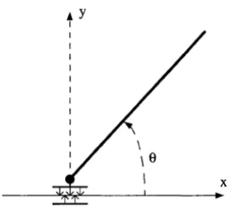
A force acts on the free extremity of the bar 2. This force remains parallel to the direction of the bar 2 and is of constant magnitude ). >

₀

(see Figure 1 . 1 ).

Figure 1.1. Geometry of the double pendulum.

• The configuration space is

JR2

equipped with its canonical structure of

coo manifold (it is not the 2-torus since the spiral springs impose to be able to count the 'number of turns'). This manifold may be represented by a single chart; in other terms, there exists a global parametrization of the system. In the sequel, we shall only use the chart

_{(q1, q2)}

defined by the angular measures associated with each of the joints.

• The kinetic energy is:

K =

This kinetic energy defines a Riemannian structure on the configuration space. The expression of the metric tensor in the considered chart is:

911 (q1' q2)

912 (q1' q2)

922 (q1' q2)

=

(�

1 +m2

)

l�,

-

�

_{m2hl2 cos (q1}

_-l)

=

921 (q1, q2),

1

₂

=

3m2l2.

• The forces mapping has for expression in the considered chart:

f(q, q; t)

=

[>.h sin {q1- q2) - (k1 + k2) q1 + k2q

2] e1(q)

+ [k2q1 - k2q2] e2(q).

The equations of motion in the chart under consideration is easily formed by use of proposition 1:

(�

+ m2) l�iP + �hl2 cos {q1- q2)

;p

+ �hl2 sin (q1- q2) (q2)2

=

Ah sin {q1- q2)- (k1 + k2) q1 + k2q2,

�hl2cos (q1- q2) i/ + !]2-l�iP- �hhsin(q1- q2) (q1)2

=

k2 (q1 - q2) .

By proposition 6, one can conclude that a unique maximal motion is associated with any initial condition. Moreover, this maximal motion is analytic and is defined for all time. Indeed, it is easily seen that there exists a positive real constant

C,

depending only on

_{(h, 12, m1, m2)}

such that:

where

1·1

denotes the canonical Euclidean norm on

JR2.

Therefore, the assump­ tions of theorem 3 are satisfied.

It should be underlined that the framework of perf ect bilateral constraints does not require that there should be no energy dissipation physically associated with a constraint. Indeed, such an energy dissipation can be described, in some cases, in terms of internal forces. For example, suppose that, in the system described above, some viscous damping with coefficients

'f/1

and

'f/2

is associated with each ball- and-socket joint. Then, it is incorporated in the forces mapping

f

which should be changed into

f(q,

q;

t)

= [-\h

sin

(q1 - q2) - (k1

+

k2) q1

+

k2q2

- ('f!l +

'f/2)

q

1

+

'f/2£i2] e1(q)

+

[k2q1 - k2q2

+

'f/2£i1 - 'f/2£i2] e2(q).

The above remark does not apply to the case of Coulomb type friction.

Remark 2. As problems II and II' are equivalent, we see that the dynamics of the constrained system depends only on the geometry of the submanifold S and not on the particular choice of the functions

'Pi

used to define it. In other words, consider a constraint, say constraint 1 , defi ne d by n functionally independent functions

'Pi

and another constraint, say constraint 2, defined by n functionally independent functions

'Pi·

Suppose, in addition, that:

S =

{q

E Q ;

Vi, 'Pi(q) = 0}= {q

E Q ;

Vi, 'Pi(q) = 0}.

Then, the dynamics of the system subjected to constraint 1 is identical to the dynamics of the system subjected to constraint 2. M oreover, the reaction forces in the motion are the same in both cases.

Since the modelling of rigid bodies system with no constraint or with per­ fect holonomic bilateral constraint leads to the constru ction of mathematical stru ctures of the same type, we state the following definition.

Definition 7 A simple discrete mechanical system is a pair

(

Q, f) where: • Q is a finite-dimensional smooth Riemannian manifold called the config­

uration manifold.

• f : TQ x lR --+ T* Q is a smooth mapping satisfying:

V(q,v)

E TQ,

V

t

E

JR,

called the forces mapping.

3. Perfect unilateral constraints

The consideration of elementary examples shows that the dynamics of rigid bodies systems can lead to some prediction of the motion where some bodies of the system overlap in the real world. Of course, this should not be allowed. Hence, very often, one has to add the statement of non-penetration conditions to a simple discrete mechanical system. This is a simple occurrence of uni­ lateral constraint. In this section, we shall discuss the consideration of perfect unilateral constraints in simple discrete mechanical systems.

3.1 The geometric description

Consider a simple discrete mechanical system with configuration manifold

Q.

A unilateral constraint is a restriction on the admissible motions of the system which is expressed by means of a finite number n of smooth real-valued functions

<pi

defined on the configuration manifold

Q:

Vi E

{1,2, . . . , n},

c.pi(q) � 0.

We denote by

A

the set of all admissible configurations:

A = _{

_q

E

Q ;

Vi E

{1,2, . . . , n},

c.pi(q)

�

0}.

( 1 .6)

The set of all active constraints in the admissible configuration

q

E

A

is defined by:

J(q)

=

{i

E {1,2,

.

.

.

, n

}

;

'Pi (q) =0}.

The following hypothesis should be brought aside regularity hypothesis I of Section 2.2.1.

Regularity hypothesis _I. The functions

<pi

are functionally independent in the sense that, for all

q

E

A, the

_dcpi(q)

(i E

_J(q))

are linearly independent in

T*Q.

Straightforward consequences of this hypothesis are: •

A

is a closed subset of

Q,

• o

A

_c

U�=1 cpi1 (

{

0

}

)

(oA is the boundary of A),

0 0

•

A= J-1 (

{0})

(A

is the interior of A).

Consider a motion

q(t)

in A and assume that a right velocity

q+ (t)

E

Tq(t)Q

exists at instant

t,

then we necessarily have:

or, equivalently,

Vi E

J(q(t)), (V<pi(q(t)), q+ (t)) q(t)

�

0,

where

V <pi ( q)

is the gradient of

<pi

at

q

defined by

V <pi ( q) =

�

( d<pi ( q)).

Thus, if the system has configuration

q

and if a right velocity

q+

exists, then

q+

necessarily belongs to the closed convex cone

V(q)

of

TqQ

defined by:

V(q)

=

_{v

E

TqQ ;

Vi E

J(q) , (d<pi(q), v)q

�

0}.

V(q)

is called the cone of admissible right velocities at the configuration

q.

In particular,

0

q

EA

(i.e.

J(q)

= 0) ==>

V(q) = TqQ.

Similarly, i f a left velocity

q-

E

TqQ

exists, then

q-

E

_{-V ( q)}

3.2 Formulation of the dynamics

The formulation of the dynamics follows the lines of MOREAU ₎ (1983, 1 988a).

3.2.1 Equation of motion. As for bilateral constraints, the realization of the constraints induces some reaction force

R.

The following hypotheses are made.

Constitutive hypothesis II. The unilateral constraints are of type contact with­ out adhesion:

V v

E

V(q), {R, v)q 2::0.

Constitutive hypothesis m. The unilateral constraints are perfect:

Vv E

{

v

E

TqQ ;

Vi E

J(q) , (d<pi(q), v)q = 0

}•

{R, v)q

=

0.

As an easy consequence of constitutive hypotheses II and m, we get:

Thus, the reaction force

R

E

T* Q

must be such that:

-R E N•(q)

�

{t,

.>.;

d<p;(q)

;

Vi E

J(q) ,

>.; � 0,

Vi�

J(q),

.>.; �

0

}·

( 1 .7)

N* (q) is a closed convex cone of T

;

Q and it is the polar cone of V(q) in the duality

(

TqQ, r

;

Q

)

. We will also have to consider the polar cone N(q) of

V (

q) for the Euclidean structure of TqQ:

N(q) �

{ t,

.1, '1 <p;(q)

; Vi

E _J(q),

A;

_;:>:

0, Vi <t

_J(q),

A;

_�

0

}

.

0

Now, consider a motion q

(t

) starting at q

o EA

at time

to

with velocity

vo.

0

Assumed to be continuous,

q(t)

remains in

A

on a right neighbourhood of

t0•

0

By formula (1.7), the reaction forceR vanishes as long as

q(t)

is in

A

and the motion is governed by the ordinary differential equation:

(q(to), q(to))

=

(qo, vo),

�

�i

=

f(q,

q; t).

Suppose that the solution of this Cauchy problem meets

8A

at some instant greater than

to.

Denote by T the smallest of these instants. The motion admits a left velocity vector

v:;.

at time T. Of course, there may happen:

v:;.

fl. V

(

q(T) ) . In this case, no differentiable prolongation of the motion can exist in

A

for

t

greater than T. The requirement of differentiability has to be dropped. An instant such T is called an instant of impact.

However, we are still going to require the existence of a right velocity vec­

tor

q+(t)

E V

(

q

(t))

at every instant

t.

The right velocity need not to be a

continuous function of time and the equation of motion

o·+

�

:

t

=

f(q,

q+; t)

+

R,

should be understood in sense of Schwartz's distribution. Actually, we require R to be a vector valued measure rather than a general distribution.

We denote by MMA{I; Q) (motions with measure acceleration) the set of all absolutely continuous motions

q(t)

from a real interval I to Q admitting a right velocity

q+ ( t)

at every instant

t

of I and such that the function

q+ (

t)

has locally bounded variation over I. Naturally, bounded variation is classically defined only for functions taking values in a normed vector space. However, for any absolutely continuous curve q(

t)

on a Riemannian manifold, parallel translation along

q(t)

classically provides intrinsic identification of the tangent spaces at different points of the curve and so, the definitions can easily be carried over to this case. The precise mathematical setting is postponed to Appendix A. The reader will notice from Appendix A that any motion q E MMA (I; Q) admits a left and right velocity,

q-

and

q+,

in the classical sense at any instant. Moreover, with any motion q E MMA(I; Q) is intrinsically associated the

covariant Stieltjes measure

Dq+

of its right velocity

q+.

The equation of motion ta es the form:

I1Dq+

=

j(q, q+; t)dt + R,

where

dt

denotes the Lebesgue measure. We have to give a precise meaning to condition ( 1 . 7) with

R

being a vector valued measure.

Convention. We shall write:

R E -N* (q(t))

to mean: there exist n nonpositive real measures

Ai

such that: n

R =

L

_{Ai d<pi(q(t)),}

i=l

V i E

{ 1 , 2, . . · , n}, Supp ).i c

{t ; <pi(q(t)) =

0}. (1 .8)

Using this convention, the final form of the equation of motion is:

R

= I1Dq+- j(q(t), q+( t) ; t) dt E -N* (q( t))

(1 .9) A straightforward consequence of the equation of motion is that an impact (that is, a discontinuity of the right velocity

_q+

by proposition 43) can only occur at an instant

t

such that

J(q(t)

::f 0. This fact is a justification for the following definition.

Definition 8 An impact occuring at time t is said simple if

_J(q(t)

contains exactly one element. If

_J(q(t))

contains at least two elements, the impact is said multiple.

3.2.2 The impact constitutive equation. We begin this section by an example. Consider the one degree-of-freedom mechanical system whose configuration space is lR equipped with its canonical Euclidean structure. The forces mapping f vanishes identically and the unilateral constraint is repre­ sented by the single function

<p1 ( q) = q

so that the admissible configuration set

A

is JR-. At initial time

to =

0, we consider an initial state

(q0, v0)

such that

qo

< 0 and

vo

> 0. It is readily seen from the equation of motion (1 .9) that an impact necessarily occurs at timet

= -qofv0•

At this time, the left velocity is

v0•

But, the right velocity can take any negative value and whatever it is, it is compatible with the equation of motion.

The reason for this indetermination lies in the phenomenological nature of the interaction of the system with the obstacle. This missing information has to be added.

Constitutive hypothesis _IV. The interaction of the system with the obstacle at timet is completely determined by the present configuration

q( t)

and the

present left velocity

q-

(

t).

In other terms, we postulate the existence of a mapping

:F

:

TQ -+ TQ describing the interaction of the system with the obstacle during an impact:

V t, q+ (t) =

:F (q(t),

q- (t)) .

( 1 . 10) To ensure compatibility with the equation of motion ( 1 .9), the mapping

:F

should satisfy:

:F (q, v-) E V(q),

:F(q,v-) - v- E -N(q).

( 1 . 1 1)

Moreover, we add the assumption that the kinetic energy of the system can not increase during an impact:

Vq E A, 'v'v- E -V(q),

( 1 . 1 2)

Let us comment on hypothesis N. When two solids hit, their bouncing is actually governed by the propagation of deformation waves in each the two solids. But, from the very beginning, we have adopted the simple framework in which each solid is supposed to be rigid, that is, for sake of simplicity, we have chosen to do not take under consideration any phenomena relying on the deformation of the solids. Thus, we cannot expect the theory to be able to predict the outcome of an impact experiment. The aim of constitutive hyposthesis N

is to introduce in the theory the missing information. Of course, in practical situations, we have to identify the unknown mapping :F. This can be done either by means of experiments or by use of a refined theory. For example, the theory of elastodynamics could be used to predict the outcome of an impact in every impact configuration. The result would be an identification of the mapping :F. In any case, there is a very big amount of work to get a precise identification of :F. This is the price we have to pay to describe sophisticated physical phenomena in a very simple framework. Actually, this issue is faced in any mechanical theory (one could think of the theory of elasticity). Naturally, in each mechanical theory, the question arises to know what amount of lacking constitutive information should be introduced. Most of the time, well-posedness of the resulting evolution problem serves as a guideline to state the constitutive hypotheses.

Definition 9 Equation ( 1.10 ), with mapping

:F

fulfilling both requirements ( 1. 11)

and (1. 12) is called the impact constitutive equation. An impact constitutive equation which ensures the conservation of kinetic energy during an impact:

There always exist many mappings F satisfying requirements (1.11) and (1.12).

Example 5. Let e : TQ -t [0, 1] be an arbitrary function. The mapping F

defined by:

(1.13)

is easily seen to satisfy requirements (1.11) and (1.12). The associated impact constitutive equation is often called the canonical impact constitutive equation. It is elastic if and only if e = 1. The function e is classically called the restitution

coefficient.

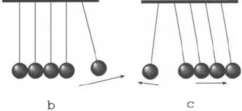
The reason why the canonical impact constitutive equation is distinguished is that in situations where only simple impact can occur (for example, if the unilateral constraint is represented by a single function cp1), then the impact constitutive equation must be the canonical one (it is a simple consequence of requirements (1.11) and (1.12)). However, in case of multiple impacts, the canonical impact constitutive equation has no specific physical relevance. A simple occurence of multiple impact is provided by Newton's cradle. The principle of the experiment is sketched on Figure 1.2.a. Its outcome is sketched on Figure l.2.b. It should be compared with the prediction of the canonical elastic impact constitutive equation which is sketched on Figure 1.2.c.

a b c

Figure 1.2. Newton's cradle.

The following proposition is a straightforward and useful consequence of requirements (1.11) and (1.12).

Proposition 10 Let F be a constitutive mapping satisfying requirements ( 1.11) and (1.12). Then, we have:

Proof. Define

v+

= F(q,

v-).

By requirement ( 1 . 1 1), we have

v- - v+

E

N(q).

Since v- E

V

(q

) n

(-V(q)),

we obtain:

(v- - v+, v-)q

=

0, that is,

(v+, v-)q

=

_{llv- 11� ·}

The use of Cauchy-Schwarz inequality and requirement ( 1 . 1 2) gives the desired

result. 0

We conclude this section by a comment on requirement ( 1 . 1 2). At first glance, it could seem to be unnecessary. The following counter-example proves that if it was omitted, then, uniqueness of solution for the resulting evolution problem would surely not hold.

Counter-example 6. Consider the one degree of freedom discrete mechanical system whose configuration space is lR equipped with its canonical structure of Riemannian manifold. The forces mapping is supposed to be constant: f

( q, q; t)

= 2. To this simple discrete mechanical system, we add the unilateral constraint described by the single function cp1

( q)

=

q.

Thus,

A

=

JR- .

The impact constitutive equation is given by formula ( 1 . 13) where the restitution coefficient is supposed to be the constant 1 /2: e(

q, q- )

= 1/2. This mechanical system is a formal description of the physical occurence of a single particle subjected to gravity and bouncing on the floor. Consider the initial instant

to =

0 and the initial state

(

q0 ,

v0

)

= (

- 1 , 0) . It is readily seen that the function

q

:

JR+

--+

JR-

defined by:

Vt

E (0, 1] ,

Vt

E (1, 2] ,

Vt

E

[3 - 2nl_l , 3 - 2�) ,

Vt

E

[3, +oo[,

q(t) = t2 -

1,

q(t) = t2 - 3t

+

2,

q(t) = t2 - (6 - 2� ) t + (3 - 2nl_r) {3 - 2� ),

q(t

₎

=

0,

(n

E N) belongs to

MMA(JR+; JR-)

and satisfies: • the initial condition,

• the equation of motion ( 1 .9) (with f

(q

,

q;

t)

= 2),

• the impact constitutive equation (1. 13) (with

e(q,

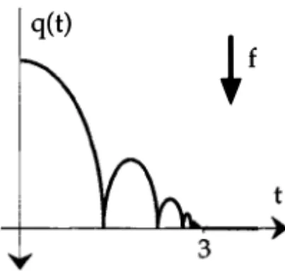
q) = 1/2).

This motion is pictured on Figure 1 .3 . Note, by the way, that it exhibits an infinite number of impacts on a compact time subinterval. It could easily be proved that no motion, defined on

[

0

,

oo

[,

with finite number of impact on every compact interval can exist.

q(t)

�f

Figure 1.3. Motion of a punctual particle subjected to gravity and bouncing on the floor.

Now, we are going to analyse what happens when the flow of time is reversed. Define q by:

1

{

[0,4]

-+

JR-q

_t

r+

q(4 - t)

Considering the initial state

(q0, v0) = (0, 0)

at

t0 = 0,

it is easily seen that

q'

satisfies:

• that initial condition,

• the equation of motion ( 1 .9) (with

f(q,q;t)

₌ 2), • the impact constitutive equation ( 1 . 13) (with

e(q, q)

= 2).

But,

q"

= 0 is also seen to satisfy the same initial condition, equation of motion and impact constitutive equation. This example demonstrates that we cannot expect uniqueness of solution when adopting the canonical impact constitutive equation ( 1 . 1 3) with restitution coefficient

e

= 2 (or any real number strictly greater than 1). But the canonical impact constitutive equation with restitution coefficient strictly greater than 1 violates requirement (1.12).

3.2.3 The evolution problem. Now, we formulate the evolution prob­ lem associated with the dynamics of rigid bodies systems with perfect bilateral and unilateral constraints. The initial condition is assumed to be compatible with the realization of the constraint:

v0 E V ( qo).

Problem m. Find

T

>

to

and

q

E

MMA([to, T[;

Q)

such that:

•

(q(to),q+(to)) = (qo,vo),

•

'Vt E [to,T[, q(t) E A,

•

R

�

bDq+ - f(q(t), q+(t); t) dt E -N*(q(t)),

The equation of motion is understood in sense of convention ( 1 .8) and the impact constitutive equation is supposed to fulfill requirements (1 . 1 1) and ( 1 . 1 2).

Yet, no regularity assumption has been made on the mapping

f.

This will be done in the next section where well-posedness of problem Ill is studied. However, we can infer from Section 1 . 1 .3 that f will be assumed to be at least of class

G1.

We can state an elementary property of any solution (if there are any) of problem Ill.

Proposition 11 (Energy inequality) Let (T,

q)

be an arbitrary solution ofprob­ lem Ill. Then, it satisfies:

Vt1,t2 E [to,T[, t1

:S:

t2,

K

(q(t2),q+(t2)) -

K

(q(h),q+(h))

=

� llti+(t2)11!(t2)-� llri+(tdll!(h) :::; r

_ltl

t2

(f

(q(s),q+(s);s) ,q+(s))q(s) ds

Proof. We have the following equality between real measures:

(q+(t) + q-(t)'Dq+)

₂

_q(t)

=

I q+(t) + q-(t)

' f

(q(t), q+(t); t)) dt + I q+(t)

+

q-(t) 'R)

0

\

2

q(t)

_\

2

q(t)

Integrating over

]t1, t2]

and using proposition 4 1 of Appendix A, we get:

Consider

D

=

{

t E]t1, t2] ; q+(t) ; q-(t)

-:/=

q+(t)} .

D is (at most) countable and therefore Lebesgue-negligible. We obtain:

�

_{11 q+ ( t2) 11 !(t2) -}

�

_{114+ ( tl) ll!(tl)}

=

rt2 (q+(t),J (q(t),q+(t);t))q(t) dt+ r 14+ ;4-,R) .

ltr

l]tl

h]

\

q

Therefore, to prove proposition 1 1 , there remains only to prove:

q +q-,R

< 0.

1

]tlh]

(

·+

2 0

)

q

But, on one hand,

r

Jq+ + q_-,R

)

=

r

(q_+,R)q = r (q_-,R)q,

1]t1,t2]\D \

2

q

_1]t1.t2]\D

_1]tlh]\D

where the second integral is nonnegative by convention (1.8) whereas the third integral is nonpositive. As a consequence:

q q

R = 0

1 (

]tth]\D

·+ + ·-

2 '

)

q .

( 1 . 1 5)

On the other hand,

r (q+(t)

+

q- (t)

R)

1

D 2 '

q(t)

r

(

q+(t)

+

_{q_-(t) , ng_+}

)

_,

1 D

2

_q(t)

�

_tED

2:

(llg_+(t) ll�ct) - lliJ-(t) ll�ct)) ,

< 0, ( 1 . 16)

by virtue of formula ( 1 . 1 2). Bringing together formulae ( 1 . 1 5) and (1.16), we

get inequality (1. 14). D

3.3 Well-posedness of the dynamics

To study the well-posedness of problem m, we need to state regularity as­ sumptions on the data. Looking at those of Section 2.2.3, we could expect to be able to prove well-posedness of problem m under the assumption that the func­ tions <fJi and the mapping f are of class

C2

and

C1

respectively. The following counter-example originally due to B RESSAN (1960) and SCHATZMAN (1978) shows that uniqueness does not hold in general even if the data are supposed to be of class coo.

Counter-example 7. Consider a simple discrete mechanical system whose configuration space is lR equipped with its canonical structure of Riemannian manifold. This is the configuration space of a particle with unit mass constrained to move along a line. A fixed obstacle at the origin is taken into consideration. It gives rise to a unilateral constraint described by the single function:

cpi(q)

=

q

Therefore, the admissible configuration set is

A

= JR-. The impact constitutive equation is supposed to be elastic. Here, the geometry is so poor that this state­ ment determines completely the impact constitutive equation. It is necessarily the canonical one with restitution coefficient e = 1 . The forces mapping f is

supposed not to depend on the state but only on time. It will be denoted by

f(t).

The initial instant is

to

=

0

and the initial state is

(qo, vo)

=

(0, 0).

The corresponding problem Ill admits here the simple formulation:

find

T

>

0

and

q E MMA([O, T[;

�) such that:

•

(q(O),q+(o))

=

(o, o), •

Vt E [0, T[, q(t)

�

0,

• R

�

dq+ - f(t) dt

is a nonpositive real measure such that:

Supp R c

{t E [0, T[ ; q(t)

=

0} ,

{

q(t)

i=

0

=>

q+(t)

=

q-(t)

•

Vt E]O, T[, q(t)

=

O

=>

q+(t)

=

-q-(t)

Here

dq+

is merely the classical Stieltjes measure associated with the func­ tion with locally bounded variation

q+.

We investigate uniqueness under the assumption that

f

is of class

coo

and nonnegative:

Vt E �+, f(t) � O.

Then, it is readily seen that the null function ij =

0

on �+ is a solution of that problem, whatever is the nonnegative

coo

function

f.

Now, we are going to construct an explicit example of such a function

f

in such a way that the associ­ ated evolution problem Ill admits another solution, distinct from the identically vanishing one.

First, define a Massin function

p

by:

p

0

{ � -+ JR. X 1---7 _{Ce z(z-1)} 1 if X

E] -

oo,

0]

U [1, +oo[ i f

x E]O,

1[ where C i s a real constant which i s chosen to get:

Define:

r+oo

}_00

p(x) dx

=

1 .

and, for every

n

E N,

00

(i + 5)2

�

(i + 1)(i + 2)(i

+

3)(i +

_{4) '}

n +

5

(n + 1)(n + 2)(n +

4)

1

fn

= n!'

1

(n

+

3)!"

(

i.e.

c5n

= �:!

(an - an+l)

)

,

Now, the functions

f(t)

and

v

(

t)

,

from [0, T[ to JR. are defined by:

f(O)

=

0

and:

Finally the function

q :

[0, T[--+ lR is defined by:

q(t)

=

lo

t

v(s) ds.

The graph of the functions

f(t)

and

q(t)

is sketched on Figure 1 .4. The reader will easily check that:

•

f(t)

is a C00 nonnegative function on [0, T[,

•

(T, q)

is a solution of the considered evolution problem,

• the only instants at which

q(t)

=

0 are 0 and the

an.

Therefore,

q

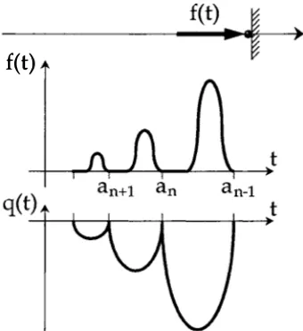
and fj provide two solutions of the evolution problem. These two solutions do not coincide on any open subinterval of (0, T[. Therefore, uniqueness of solution for problem m cannot be asserted, even in the case

where the data are supposed to be of class 000• PERCIVALE ( 1 985, 199 1 ) was the first to notice that, in the above example, if f

( t)

is supposed to be analytic, then uniqueness of solution does hold. Recently, a complete discussion of the one-degree-of freedom problem was obtained by S cHATZMAN ( 1 998). The general case is treated in BALLARD (2000) and is now recalled. Let us just mention that prior existence results had been obtained, but they were limited to the case where the unilateral constraint is represented by a single function (see

MONTEIRO MARQUES ( 1 993) and S CHATZMAN ( 1 978)).

f(t)

f(t)

.

i

Figure 1.4. Bressan-Schatzman counterexample.

Regularity hypothesis V. The Riemannian configuration manifold, the func­ tions

'Pi

and the mapping f :

T

Q x

lR --+

T* Q are analytic.

The proof of the following proposition can be found in BALLARD (2000). An earlier proof can also be found in LOTSTEDT ( 1982).

Proposition 12 Let

_qo

E

A

and

vo

E

V(qo).

Then, there exist

Ta

>

to

, an analytic curve

_{qa : [to , Ta [--+}

Q and n analytic functions

Aai : [to, Ta [--+ lR

such that: