A simplified method to account for the non linearity of aerodynamic coefficients in
the analysis of wind-loaded bridges
Vincent Denoël1, Hervé Degée1
1University of Liège, Department of Mechanics of materials and Structures
Chemin des Chevreuils, 1, B-4000 Liège (Belgium) email: V.Denoel@ulg.ac.be, H.Degee@ulg.ac.be
Abstract – Based on a non linear quasi-steady wind model, this paper presents the statistical characteristics of the wind loading. These statistical characteristics are computed in an analysical way and validated thanks to a Monte Carlo sim-ulation. After this validation, a parametric study allows giving some general observations concerning the non Gaus-sianity of the loading. Statistical moments up to the fourth order are computed in an analytical way. The subsequent relations are expressed as a function of the slope and curva-ture of the aerodynamic coefficients. They are a usefull tool for the assessment of the non Gaussianity of the wind load-ing on any bridge deck. This is illustrated for three famous European bridges.
Keywords – Wind engineering, Non Gaussianity, Quasi-steady wind loading, buffeting, aerodynamic coefficients
I. Introduction
T
HE complete interaction between a bridge’s motion and the oncoming flow is so complex that the design procedure of a bridge deck subjected to a wind loading is commonly limited to some checkings. For each of them a particular loading model has to be considered ([2]).For example, some complex loading models including transient effects are usually used for the investigation of the self-excited phenomena ([12]). Even if these wind loading models seem to be sophisticated because of their expression in terms of convolution integrals and admittance functions, the basic expression of this loading is composed of linear terms and based on a superposition principle.
Another set of checkings concerns the response of the structure to buffeting forces. For the sake of simplicity in mathematical models, the model is very often considered as linear. This excludes any estimation of the non linear ef-fects of the loading. These effects can come either from the non linearity of the aerodynamic coefficients or from the non linearity of some geometric relations used to express the wind velocity and the wind angle of attack ([5]). Some previous researches ([1], [2], [7], [9]) aimed at estimating the effects of this second kind of non linearity. The main conclusions are recalled and presented in this paper. Based on the same kind of developments, the effects of the non linearity of aerodynamic coefficients are presented in this document. It has already been shown ([6]) that important discrepancies occur in a 2-D turbulent wind flow. So, con-trarily to the previous researches, the context of this paper concerns a 2-component wind field instead of a single 1-D flow.
The main goal of this paper is thus to show the effects of the non linearity of aerodynamic coefficients. As a first step it seems quite logic to investigate the influence on the aerodynamic force. Then the influence on structural dis-placements, internal forces and eventually stresses could be
Fig. 1. Examples of aerodynamic coefficients considered. This paper is mainly devoted to the first step which is the most important in practical application since the statistical characteristics of structural displacements can often be expressed as a function of the statistical char-acteristics of the forces.
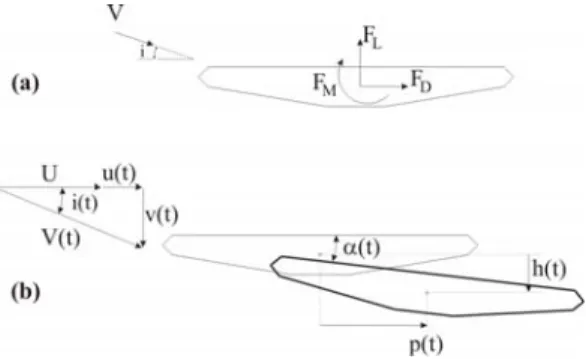
II. The non linear quasi-steady wind loading Forces acting on a body immerged in a fluid result from the normal pressures acting on it. In civil engineering appli-cations, and more particularly in bridge engineering, three forces (drag, lift and moment) are generally considered. For example, the aerodynamic drag force acting on a fixed body in a uniform flow with constant velocity V can be expressed by ([12]):
FD=
1
2ρCDBV
2 (1)
where ρ and B represent respectively the air density and the width of the body, i.e. the bridge deck. In usual ap-plications, the aerodynamic coefficients (CD, CL and CM)
exhibit (see Fig. 1) a significantly non linear dependency with respect to the wind angle of attack, i.e. the angle between the wind direction and the bridge deck (see Fig. 2). This angle remains however small (i- 15◦) which al-lows deriving a Taylor series expansion of the aerodynamic coefficient:
CD(i) = c0+ c1i +
c2
2!i
2+ ... (2)
Civil engineering structures are built in the atmospheric boundary layer. In this region the wind flow is known to be turbulent. It is composed of a mean velocity U and lon-gitudinal u(t) and transverse v(t) fluctuations which are
Fig. 2. (a) Aerodynamic forces in a uniform flow ; (b) Components of turbulence and displacements of the deck
generally modelled as Gaussian stochastic processes ([12]). Davenport proposed to express the forces acting on a struc-ture immerged in such a turbulent flow by the same relation ([4]):
FD(t) =
1
2ρCD[i (t)] BV
2(t) (3)
where both the wind angle of attack and the squared wind velocity are now time-dependent. It is commonly ac-cepted that this well known quasi-steady wind model is suit-able for representing bridge vibrations at lower (reduced) velocities ([2]). Based on geometric relations derived from Fig. 2, these two quantities can be expressed as a function of the bridge motion (h, p, α) and of the components of the turbulence, which results, for the loading (Equ. 3), in a non linear function of Gaussian processes u(t) and v(t).
As illustrated in § III-A, a non linear function of Gaussian processes provides a non Gaussian process which is much less convenient to handle than a Gaussian one. On the contrary, a linear function of Gaussian processes remains a Gaussian process ([3]).
Because of the need to work with a simple model, the rig-orous expression of the loading is thus very often linearized. This is achieved by linearizing:
• the aerodynamic coefficient (CD(i) = c0+ c1i); • the non linear geometric relations for i (t) and V (t).
Some previous researches ([1], [2], [7], [9]) have already investigated the effects of this second item. Based on a quadratic expression of the loading, they have shown that the non linearity coming from the geometric relations could lead to an inaccurate representation of the loading. In this paper, the influence of both non linear origins will be con-sidered. The development of the non linear relation (3) up to the second order, including both items and written now in a non dimensional form, gives ([5], [6]):
f (t) = 1FD(t) 2ρc0BU2 = 1 + 2u U + c1 c0 v U | {z } (I) +u 2 U2+ c1 c0 uv U2 + v2 U2 | {z } (II) + c2 2c0 v2 U2 | {z } (III) (4) -150 -10 -5 0 5 10 15 0.02 0.04 0.06 0.08 0.1 0.12 I I+II I+II+III
Fig. 3. Probability density function of the loading under several levels of hypotheses
Keeping terms (I) and (II) of this relation degenerates in studying the effects of the previous researches, i.e. the second item only, whereas keeping the first term only (I) corresponds to the most usual linearization of the loading. Factor c2 in the third term (III) shows clearly that this
term aims well at accounting for the non linearity of the aerodynamic coefficient.
It is important to note that the non linearity of the aero-dynamic coefficient appears trough transverse effects only (v2) which indicates that accounting for the non linearity
of aerodynamic coefficients has no sense in a 1-D flow. This is the main reason for which the previous researches, often limited to 1-D flows, did not care for this particular non linearity.
III. Non Gaussianity of the wind loading A. Illustration by Monte Carlo simulation
In order to illustrate the non Gaussianity caused by the non linear quasi-steady loading, a Monte Carlo simulation of the non dimensional forces has been realized. The exam-ple is illustrated with the moment coefficient of the Nor-mandie Bridge. For this particular aerodynamic coefficient, the coefficients of the Taylor series expansion (2) are:
c0= 0.0263 ; c1= 0.973 ; c2= −3.50 (5)
Concerning the characteristics of the wind velocity, it is supposed that the mean wind velocity is U = 10m/s and that the standard deviations of both components of the turbulence are σu= σv= 1m/s. This corresponds to a
10%-intensity which lies in the expected order of magnitude for practical applications.
The Monte Carlo simulation is achieved by generating a long Gaussian sample (N = 500000 points) for each com-ponent of the wind turbulence. Based on the quadratic expression of the non-dimensional loading (4), three forces corresponding to each level of hypothesis (I, I + II and I + II + III) are then computed. The histograms of these simulated forces are finally used as estimates for the corre-sponding probability density functions (Fig. 3).
As announced previously, the force computed with the linear model (I only) results in a Gaussian probability func-tion. It can be easily identified on Fig. 3. Accounting for
TABLE I
Statistical moments of the non dimensional loading (Monte Carlo simulation)
Model Mean Std Skewness Excess
I 1.0010 3.7008 0.0044 0.0078
I + II 1.0209 3.7189 0.0523 0.1220
I + II + III 0.3574 3.8292 −0.9679 1.3849
the non linearity coming from the geometric relations (I and II) does not bring any significant modification. How-ever when the non linearity of the aerodynamic coefficient is included in the simulation (I, II and III), the resulting probability density function is clearly skewed to the left. This indicates a more frequent occurrence in the range of large (in absolute value) negative values and hence an ob-vious impact on the design values.
In figure 1 it can be seen that the linear approximation of the considered aerodynamic coefficient is above the actual curve for positive angles of attack and under for negative angles. So when the wind angle of attack varies, the non linear aerodynamic coefficient varies in a range which is "shifted down" compared to what would be obtained with a linear model. This is the physical justification for the negative skewness of the resulting force.
A more precise idea of the actual non Gaussianity of the forces generated with all three methods can be obtained by computing the statistical moments. They are reported in table I. The minor difference between loadings I and I + II can again be observed; also the non Gaussianity of the third force is obvious by looking at the skewness and excess coefficients. It should be noticed that the mean value is also considerably affected by the non linearity of the aerodynamic loading, which could less easily be stated by looking at probability density functions only.
B. Analytical developments
The Monte Carlo simulation is interesting because it does not require any complex computation and leads easily to significant results. The main drawback of this method is its high demand in computational time. Since very long samples are needed to reproduce accurately the high order moments, this argument is again strengthened when non Gaussian processes are studied. For this reasons, and be-cause it would be desired to realize a parametric study, it is interesting to derive some analytic developments. Based on the theory of probabilities, the statistical moments (up to the fourth order) of the quadratic expression of the force given in Equ. (3) can be computed in a analytical way ([5]):
TABLE II
Statistical moments of the non dimensional loading (Analytical approach)
Model Mean Std Skewness Excess
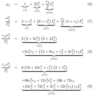
I 1 3.7043 0 0 I + II 1.0200 3.7227 0.0481 0.1196 I + II + III 0.3553 3.8361 −0.9721 1.4189 µf = 1 |{z} (I) + 2Iu2 |{z} (II) +r2 2I 2 u | {z } (III) (6) σ2 f I2 u = 4 + r21 | {z } (I) +¡6 + r21¢Iu2 | {z } (II) +r2 2 (4 + r2) I 2 u | {z } (III) (7) γ3σ3 f I4 u = 2¡4 + 3r12¢ ¡3 + 2Iu2¢ | {z } (II) +3r12r2+ ¡ 12 + 6r2+ r22+ 3r21 ¢ r2Iu2 | {z } (III) (8) γeσ4 f I6 u = 6¡16 + 24r12+ r14¢ ¡2 + Iu2¢ | {z } (II) +96r21r2+ 12r12r22+ (96 + 72r2 +24r22+ 72r21+ 3r23+ 12r12r2 ¢ r2Iu2 | {z } (III) (9)
where Iu = σuU represents the intensity of the wind
ve-locity and r1 = c1c0 and r2 = c2c0 are the ratios of higher
coefficients of the Taylor series expansion to the mean aero-dynamic coefficient. These ratios will be used in the fur-ther developments as indicators for the non Gaussianity of the quasi-steady aerodynamic loading. For the sake of simplicity, the above equations have been derived under the assumption of equal turbulence intensities and uncor-related components of turbulence. More general results can be found in ([5]).
From numerical values associated to the considered aero-dynamic coefficient (Equ. 5), ratios r1 and r2 can be
es-timated (r1 = 36.99 and r2 = −132.95) and then used
for the computation of the statistical characteristics of all three loadings. Results are reported in Table (II).
The agreement with numerical values presented in Table (I) gives another important interest to the Monte Carlo simulation: its efficacy to validate other (e.g. analytical) models. Reversely thinking, the good agreement shows that 500000-data samples are sufficient to reproduce cor-rectly the fourth order statistics.
Exactly as extreme values of Gaussian processes can be expressed by the product of the standard deviation and a peak factor ([3]), some mathematical models represent the extreme value statistics of non Gaussian processes as func-tions of skewness and excess coefficients ([8], [11]). Since the developments presented in this paper aims at
determin-ing easily the statistical moments of the loaddetermin-ing, relations (6) to (9) are thus the necessary tools to estimate, thanks to these models, the statistics of extreme values which are needed to realize the final design of a structure.
IV. Parametric study of the loading If the turbulence intensity is fixed (Iu= 10% in the
fol-lowing), right-hand sides of equations (6) to (9) are simple functions of parameters r1 and r2. This paragraph aims
at determining, as a function of these two parameters, the effects of the non linear terms of the loading (II and III) on each statistical moment.
A. Influence on the mean A.1 Influence of II
For usual values of the wind intensity (∼ 10%) Equ. (6) shows that the non linear term (II) brings at most a 2%−variation of the mean force, regardless the considered aerodynamic coefficient.
A.2 Influence of III
Contrarily, because r2 can be very large in absolute
value, the non linearity of the aerodynamic coefficient (III) can drastically modify the mean force. Depending of the sign of r2, the mean force can be increased (r2 > 0) or
decreased (r2 < 0). This was clearly illustrated with the
moment coefficient of the Normandie Bridge. B. Influence on the standard deviation B.1 Influence of II
Equation (7) shows that the ratio of the contribution of (II) to the variance to the contribution of (I) is expressed by: ¡ 6 + r2 1 ¢ I2 u 4 + r2 1 (10) which lies between I2
uand 1.5Iu2. This indicates that the
term (II) does not bring any significant modification to the variance neither and explains why the previous researches ([1], [2], [7], [9]) stated that the non linearity of the loading (limited to term II) does not affect significantly the first two statistical moments. With this kind of non linear term of the loading, attention should be paid to the third and fourth order moments only.
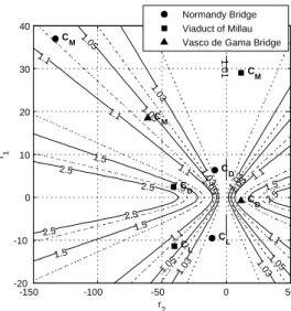
B.2 Influence of III
The ratio of the total variance (I + II + III) to the contribution of (I) only is a function of both r1 and r2.
It is represented in figure 4. Contrarily to what could be observed with term (II) only, this figure shows that the difference can be as large as 250%! For a given value of the curvature of the aerodynamic coefficient r2, the
discrep-ancy is much more important when the ratio r1 is small.
This condition concerns thus mainly the drag coefficients. As an illustration, couples (r1, r2) for the aerodynamic
coefficients of Fig. 1 are reported on this figure. It can be checked that the variance of the actual drag force expected for the Viaduct of Millau (i.e. including the non linearity
1 .0 1 1.03 1 .0 3 1.03 1.03 1.0 3 1.05 1.05 1.05 1.05 1.05 1.05 1.1 1.1 1.1 1.1 1.1 1.1 1.5 1.5 1.5 1.5 1.5 2.5 2.5 2.5 2.5 2.5 r 2 r1 CD CL CM C D CL C M CD CM -150 -100 -50 0 50 -20 -10 0 10 20 30 40 Normandy Bridge Viaduct of Millau Vasco de Gama Bridge
Fig. 4. Ratio of the variance of the aerodynamic force obtained with (I + II + III) to the variance obtained with (I) only − Iu= Iv= 10%
of the loading) is for example 1.8 times higher than what would be obtained with the linear approach.
Some developments based of on Equ. (7) show that the curvature of the aerodynamic coefficient decreases very rarely the standard deviation of the aerodynamic force: it is actually limited to the case −4 < r2< 0.
C. Influence on the skewness coefficient C.1 Influence of II
Because of the Gaussianity of the linear counterpart of the loading, the skewness of the aerodynamic force comes from terms II and III only (see. Equ. (8)). For small intensities of turbulence, the skewness coefficient related to the term II is proportional to this intensity:
γ3'6 ¡ 4 + 3r2 1 ¢ (4 + r2 1) 3/2Iu (11)
which starts with γ3 = 3Iu at r1 = 0, reaches a
max-imum value γ3 ' 4.2Iu at r1 = 2 and then decreases to
0 for higher values of |r1|. This is illustrated in Figure 5
where horizontal contour lines indicate a dependency to r1
only. Skewness coefficients resulting from this first kind of non linearity can thus rise up to γ3 ' 0.5 which is
actu-ally large enough to modify significantly the statistics of extreme values ([11]).
It is important to note that the skewness generated by this kind of non linearity can lead to positively-skewed probability density functions only. No negative skewness coefficient could be justified.
In our practical application, the skewness coefficient is rather low (γ3' 0.0481, see Table II). This is due to a large r1 ratio which is often the case for moment coefficients.
Figure 5 shows that large skewness coefficient should rather be expected for drag coefficients.
0.1 0.1 0.1 0.1 0.1 0.1 0.2 0.2 0.2 0.2 0.2 0.2 0.3 0.3 0.3 0.3 0.3 0.3 0.3 0.3 0.3 0.3 0.3 0.3 0.4 0.4 0.4 0.4 0.4 0.4 0.4 0.4 0.4 0.4 0.4 0.4 r 2 r1 CD CL CM C D CL C M CD CM -150 -100 -50 0 50 -20 -10 0 10 20 30 40 Normandy Bridge Viaduct of Millau Vasco de Gama Bridge
Fig. 5. Skewness coefficient of the loading obtained with term II only − Iu= Iv= 10%
C.2 Influence of III
The curvature of the aerodynamic coefficient can affect drastically the skewness coefficient of the loading. This is illustrated at Fig. (6) where the new shapes of the contour lines exhibit a main dependency to r2. As expressed
pre-viously with a physical interpretation (based on "shifted intervals") the skewness coefficient of the loading is neg-ative for negneg-ative r2 ratios (curvature of the aerodynamic
coefficient to the bottom). On the contrary, the probability density function of the loading is skewed to the right for positive r2 ratios.
For the chosen aerodynamic coefficient (CM in the upper
left corner) the skewness coefficient is equal to −0.97, which was observed to be sufficient to require a modified proce-dure for the estimation of design values ([8]). Note that the standard design procedure ([12]) devoted to the estimation of extreme values holds for Gaussian processes only. In this sense, a clever design of a bridge deck would consist in try-ing to place the characteristics points (r1, r2) in the area
of small-valued contour lines. This is for example achieved for the drag and lift coefficients of the Normandie Bridge. D. Influence on the excess coefficient
D.1 Influence of II
Similarly to what could be observed at the third order, no contribution to the fourth order moment is brought by the first (linear) term of the aerodynamic loading. If terms related to the first kind of non linearity only are kept, the excess coefficient of the loading can be estimated by:
γe' 12
16 + 24r21+ r14
16 + 8r2 1+ r14
Iu2 (12)
which lies between γe = 12Iu2 and γe = 24Iu2. This
ap-proximation is limited to small wind intensities. The exact excess coefficient derived from Equ. (9) is represented in Fig. (7). For a 10%-intensity it can be checked that a good agreement is obtained with the approximate value given by Equ. (12). -2 .6 -2.2 -2.2 -2.2 -1.8 -1.8 -1.8 -1.8 -1. 4 -1 .4 -1.4 -1.4 -1 -1 -1 -1 -0 .6 -0 .6 -0.6 -0 .2 -0 .2 -0.2 0 .2 0.2 0.2 0.6 0.6 0.6 1 1 1 1.4 1.41.8 r 2 r1 CD CL CM C D CL C M CD CM -150 -100 -50 0 50 -20 -10 0 10 20 30 40 Normandy Bridge Viaduct of Millau Vasco de Gama Bridge
Fig. 6. Skewness coefficient of the loading obtained with terms II and III − Iu= Iv= 10%
Again drag coefficients, or more generally aerodynamic coefficients with small r1 ratios, seem to suffer much more
from the non Gaussianity of the loading.
The non linear loading model is quite limited because it leads to excess coefficients lying in a narrow band [12I2
u, 24Iu2], narrower at least than what could be expected
in practical measurements ([8]). In the context of small wind intensities, this model does not provide noteworthy excess coefficients. This is why the non linear model lim-ited to term II is often mainly devoted to determining the third order statistical characteristics.
D.2 Influence of III
Figure (8) shows the excess coefficient obtained with the non linear loading model including the non linearity related to the aerodynamic coefficient. The significantly different shapes of the contour lines of Figs (7) and (8) indicate that the r2ratio can influence significantly the excess coefficient.
With this kind of model, the excess coefficient can rise up to more than 10! This affects also significantly the statistics of extreme values.
Since the contour lines derived for the fourth order mo-ment analysis (8) have almost the same shape as the con-tour lines derived for the third order moment analysis (6), the same kind of reasoning is also valid concerning a clever design of the bridge deck.
V. Computation of structural displacement, stresses, etc.
Even if it is important to describe the loading as pre-cisely as possible, designers are however mainly interested in determining the structural displacements, internal forces and stresses. The determination of such quantities is not necessarily obvious since the equation of motion with non deterministic right-hand side has to be solved in a proba-bilistic way, up to the fourth order.
0.15 0.15 0.15 0.15 0.15 0.15 0.15 0.15 0.15 0.15 0.15 0.15 0.2 0.2 0.2 0.2 0.2 0.2 0.2 0.2 0.2 0.2 0.2 0.2 r 2 r1 CD CL CM C D CL C M CD CM -150 -100 -50 0 50 -20 -10 0 10 20 30 40 Normandy Bridge Viaduct of Millau Vasco de Gama Bridge
Fig. 7. Excess coefficient of the loading obtained with term II only − Iu= Iv= 10% 2 2 2 2 2 2 4 4 4 4 4 4 6 6 6 6 6 8 8 8 10 10 r 2 r1 C D C L C M CD C L C M C D C M -150 -100 -50 0 50 -20 -10 0 10 20 30 40 Normandy Bridge Viaduct of Millau Vasco de Gama Bridge
Fig. 8. Excess coefficient of the loading obtained with terms II and III − Iu= Iv= 10%
A. Rigorous approach of the response
For example, the second order characteristics of a ran-dom loading are represented by its power spectral density which represents the distribution in the frequency domain of the variance of the process. The frequency content of the response, i.e. its power spectral density, can be obtained by multiplying the power spectral density of the force by the squared transfer function of the single degree of freedom system. The surface under the resulting function (function of the frequency) is equal to the variance of the response.
At the third order, the same kind of reasoning holds: the third order moment of the response is obtained by nu-merical integration of the corresponding bispectrum. This quantity is a 2-D function of frequency parameters which represents the frequency distribution of the third order mo-ment. It is obtained by the multiplication of the bispectrum of the force and the 2-D transfer function, more commonly called the second order Volterra kernel ([5]).
The fourth order characteristics of the response can be established following an identical procedure but working now with a supplementary dimension: the trispectrum (dis-tribution of the fourth order moment in a 3-D frequency space) of the response can be obtained by multiplying the trispectrum of the force by a third order Volterra kernel. B. Approached methods
In practical applications, this rigorous approach is rarely applied. This is mainly due to historical developments: at the very beginning of wind engineering (early sixties), com-putational means were not comparable to today’s means. Based on a white approximation, Davenport ([4]) proposed a simplified procedure which allows avoiding the numeri-cal integration required for the computation of the second order response. Because of its high efficiency and accu-racy ([5]), this method, based on the decomposition of the response into a background and a resonant component, is nowadays still very common.
The decomposition of the response into a background and a resonant contributions is also attractive in the con-text of non Gaussian processes. Indeed, since the back-ground counterpart is nothing else than a static transfor-mation of the loading, it has the same non Gaussian struc-ture: same skewness and excess coefficients. On the other hand, because of its dynamic (i.e. harmonic) type, the resonant counterpart can be considered as a Gaussian con-tribution.
Depending on the dispatching of the total energy into the background or resonant contributions, the response could be more or less Gaussian. Both extremes are:
• a Gaussian response if the resonant counterpart is
dom-inating;
• a non Gaussian response with the same skewness as the
loading is the background counterpart is dominating. Based on the actual dispatching of the total energy into both contributions, references (??) and (??) present some interpolation functions which allow giving good estimates for the statistical characteristics of the structural response.
VI. Conclusions
In this paper, the non linear quasi-steady model has been considered. The main scope was to enlighten the influence of the non linearity on the statistical characteristics of the loading. Under the assumptions of uncorrelated compo-nents of turbulence (u(t) and v(t)) and equal turbulence intensities (Iu = Iv), analytical relations have been
com-puted for the first four statistical moments of the non linear loading. Two distinct non linear contributions can be dis-tinguished in this model:
• non linear terms related to non linear geometric relations.
They have been already widely studied in a 1-D turbulence field (v(t) = 0). In this paper, investigations have been considered in a 2-D flow. It has been shown that:
— this first kind of non linearity does not affect signifi-cantly the mean and standard deviation of the loading;
— it could lead to positive skewness coefficients (only!) up to approximately 4.2Iu, which remains small but sufficient
to have to consider a non Gaussian model for the estimation of extreme values;
— concerning the fourth order moment, the influence is limited to 24I2
u and could thus eventually be neglected in
many applications;
• non linear terms related to the non linearity of the
aero-dynamic coefficients. It was shown that these terms arise in 2-D turbulence fields only. Their influence on the sta-tistical moments of the loading is more complex and was quantified as a function of the slope (c1) and curvature (c2)
of the aerodynamic coefficient. It was shown that:
— the mean force can be increased (if c2/c0 > 0) or
de-creased (if c2/c0< 0) significantly. This is important since
extreme values used for the final design are expressed by reference to mean values;
— the standard deviation is most often significantly in-creased. A reduction of the standard deviation is not impossible but happens when a strict condition on the mean aerodynamic coefficient and its curvature is satisfied (−4c0< c2< 0);
— the skewness coefficient has got (approx.) the same sign as c2/c0 and could thus be positive or negative, which is
more realistic. Moreover, values as large as γ3 = ±2 can be obtained with this model;
— the excess coefficient could be 50 times larger as what would be obtained with the first kind of non linearity only. A special attention should be paid to the estimation of extreme values when the skewness and excess coefficients indicate a non Gaussianity. In this case, the statistics of extreme values can be derived as a function of these two coefficients ([8]). The analytical relations provided in this paper are thus the necessary tools to estimate the extreme values of the non linear loading.
Thanks to a parametric study, it has been illustrated that, because of a usually small c1/c0ratio, the drag
coef-ficients suffer much more from the non Gaussianity. As an endpoint, some general comments have been for-mulated concerning the estimation of the statistical char-acteristics of the structural response. Thanks to the usual decomposition of the response into a background and a resonant contribution, the non Gaussianity of the response can be assessed very easily. The existence of a mitigating effect of the resonant counterpart results in smaller skew-ness and excess coefficients for the response than for the loading. Because estimates for the skewness and excess coefficients are available, this allows thus estimating the design displacements, internal forces, stresses, etc.
Acknowledgments
The authors would like to warmly acknowledge the Bel-gian National Fund for Scientific Research for having given a financial support to this research.
References
[1] Benfratello S., Di Paola M., Spanos P.D., Stochastic response of MDOF wind-excited structures by means of Volterra series approach. Journal of Wind Engineering and Industrial Aerody-namics, Vol 74, 1135-1145, 1998.
[2] Chen X., Kareem A., Advances in modelling of aerodynamic forces on bridge decks. Journal of Engineering Mechanics, Vol 128-11, 1193-1250, 2002.
[3] Clough R.W., Penzien J., Dynamics of Structures, Mc Graw-Hill : Civil Engineering series (second edition), 1993.
[4] Davenport A.G., The application of statistical concepts to the wind loading of structures, Proceedings of the Institute of Civil Engineers, Vol 19, 1961
[5] Denoël V., Application des méthodes d’analyse stochastique à l’étude des effets du vent sur les structures du génie civil, PhD thesis, University of Liège, Belgium (in french), 2005.
[6] Denoël V., Non Gaussian response of bridges subjected to tur-bulent wind-effect of the non linearity of the aerodynamic coef-ficients, Proceeding the the 3rd European Conference on Com-putational Mechanics, 2006
[7] Grigoriu M., Response of linear systems to quadratic gaussian excitation, Journal of Engineering Mechanics ASCE Vol 112(6) 729-744, 1986.
[8] Gurley K., Tognarelli A., Kareem A. Analysis and simulation tools for wind engineering, Probabilistic Engineering Mechanics, Vol 12(1), 9-31, 1997.
[9] Kareem A.and al., Modelling and analysis of quadratic term in the wind effects on structures. Journal of Wind Engineering and Industrial Aerodynamics, 74, 1101-1110, 1998.
[10] Lutes L.D., Hu S.L., Non normal stochastic response of linear systems, Journal of Engineering Mechanics, ASCE, Vol 112, 127-141, 1986.
[11] Soize C., Kree P., Mécanique aléatoire, Ed. Dnod, Paris, 1983. [12] Simiu E., Scanlan R.H, Wind effects on structures, John Wiley