Combined simulation of the building, primary and secondary plant of a typical office building

(1)

8th International Conference on System Simulation in Buildings, Liege, December 13-15, 2010

Combined simulation of the building, primary and secondary

plant of a typical office building

B. Fabry

1

, V. Dolisy

1

, P.-Y. Franck

1

, S. Bertagnolio

2

, P. André

1

(1)

Building Energy Monitoring and Simulation Research Unit, University of Liège, Arlon campus, Belgium

(2)

Thermodynamics Laboratory, University of Liège, Belgium

ABSTRACT

Office buildings are very often equipped with complex HVAC systems made of primary, secondary and control sub-systems. The interaction between those elements is complex and requires specific analysis tools. In the context of the IEA-ECBCS Annex 48 and IEE-HarmonAC projects, a typical office building of the Walloon region was deeply analyzed through both monitoring and simulation work.

The main objective of the work was, starting from the existing status of the building, to assess the performance of a number of changes in the building envelope, HVAC system and control system. In particular, the performance of different reversible (air coupled, ground coupled) heat pumps was calculated and compared to a reference situation (separate production for heating and cooling).

To achieve this objective, different simulation tools were used. This paper will relate the development, calibration and use of a detailed TRNSYS application integrating a multi-zone (10 per floor) modeling of the building envelope, a detailed representation of the secondary plant (including the simulation of a customized VAV system), a modeling of the different configurations of the primary plant (with and without heat pump) as well as a realistic consideration of the main elements of the control system.

The paper will present successively the architecture of the simulation application, the selection of the Types required to perform the task, the calibration of some of them using measurements carried out in the building and the results obtained by running a number of configurations of the system.

The paper will specifically focus on the problems generated by the interaction between the primary and secondary plant as well as with the specific issues related to the simulation of the control system.

(2)

1. INTRODUCTION

Based on the work performed for IEA-ECBCS Annex 48 and IEE-HarmonAC projects, this paper aims at presenting the development of a complete dynamic simulation of a typical office building, including its primary and secondary plant.

The methodology was as follows: using a multi-zone building definition, climate data and a primary system type, the behavior of the complete system is simulated. It includes the primary system, the air handling unit, heating and cooling coils, hydraulic and aeraulic networks, controllers…

This work was also meant to verify and confirm the simulation results obtained with a specific EES-based tool developed for IEA-ECBCS Annex 48 project: AHPSAT1. This tool was used to evaluate the energy consumptions and savings for different heating and cooling systems, given the hourly heating and cooling demands. These demands can be provided by measurements or by another TRNSYS simulation, in which the multi-zone building only would be simulated.

However, as AHPSAT doesn’t take the secondary system into account, a global simulation in TRNSYS was necessary, to understand in which way the secondary system may increase the overall consumption, in the particular case of this office building in Belgium. 3 different primary system configurations will be studied in this paper: the actual one (separated heating and cooling production), and two reversible systems, one of which is coupled with a geothermic exchanger.

The conclusions of these simulations will be the basis of a proposition for the retrofit of the existing building.

2. BUILDING AND SYSTEM PRESENTATION

2.1. The building

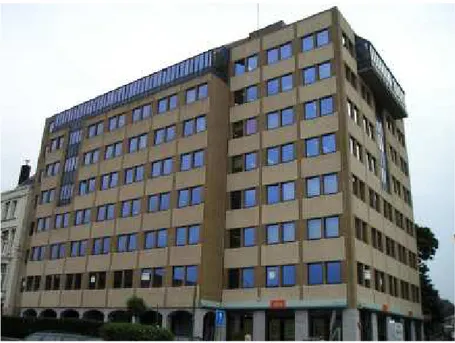
The simulated building is a medium size office building built in Charleroi at the end of the eighties. As it can be seen on figure 1, it is a 9 storey building with about 7 220 m² of air-conditioned offices and meeting rooms as well as 3 levels of parking lots. A four storey zone of the building for which energy balances can be worked out has been identified (floors 4, 5, 6 and 7). About 40 people occupy each of these floors from 8 AM to 6 PM, 5 days per week, all year long.

The external walls are composed of prefab concrete boards with a thin insulation layer (3 cm of mineral wool). The global U value is about 1 W/m²K. The windows are made of a classical double glazing (U = 2,84 W/m²K, g = 0,8).

1

More info about this software and downloadable versions can be found on the website of Thermodynamics Laboratory of University of Liège: http://www.labothap.ulg.ac.be/cmsms/

(3)

8th International Conference on System Simulation in Buildings, Liege, December 13-15, 2010 Figure 1: building of interest

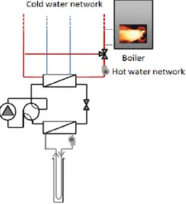
2.2. The secondary system

The existing secondary system is « all air » type. Figure 2 below represents the air handling unit. The return air is mixed with some fresh air (minimum 25%) and passes through a filter, a pre-heating coil, an adiabatic humidifier and a cooling coil. The supply temperature set point is almost constant during the whole year: 14°C. The air is then circulated through a duct network to local post-heating coils (7 or 8 post heating coil for one floor). Each post-heating coil can supply up to 5 VAV boxes, so that the occupants can adapt the local comfort conditions (+/- 2°C) around 21°C. All the post-heating coils are supplied with hot water from the primary system.

(4)

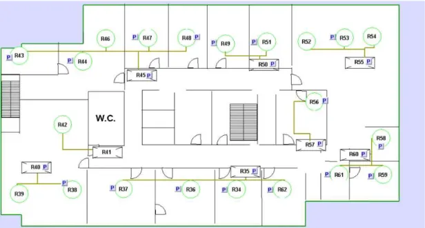
Figure 3: a typical floor with post-heating coils (black rectangles) and VAV boxes (green circles)

3. THE SIMULATION SCHEME

3.1. General assumptions

For simulation purpose, only one floor was simulated in TRNSYS. Indeed, the structure of the floors is quite similar if we neglect some specific rooms with high internal gains (computer room for example). The storey was divided into ten thermal zones, as shown by figure 4. The zones number 2 and 10 are not air-conditioned.

(5)

In order to simplify the control, the inside temperature set points are 21°C in winter and 23°C in summer. The possibility to adjust this set point by the occupants was not taken into account. Some hysteresis has to be added in different parts of the control system, in order to ensure numerical convergence of the simulation.

Figure 5 represents the architecture of the TRNSYS simulation of the systems. Given the complexity of the system, it includes a number of macro-types for many parts of the system: Air Handling Unit (“GP2”), chiller and boilers (“Primary System”), post heating coils and terminal units (“Post-Heat VAV”), post heating boxes controllers (“Control_Box_Post-Heat”), building (“Building”), valves (“Collector Valves”) and aeraulic networks (“Transit In” and “Transit Out”). They will be discussed in the next section.

Figure 5: TRNSYS general simulation scheme

3.2. Simulation components

3.2.1. Air Handling Unit (“GP2”)

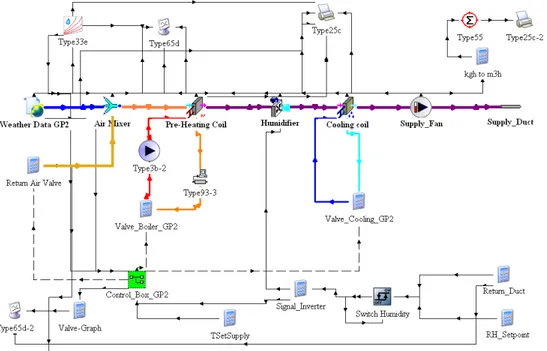
The Air Handling Unit macro contains all the elements described in section 2.2., as well as another macro which handles all the control strategy. Given the minimum fresh air ratio, the return air temperature and relative humidity, the AHU has to produce 14°C air. To achieve this set point, the pre-heating coil (TRNSYS type 753) is supplied with water at constant flow rate but with adapted temperature. The humidifier (type 641) ensures that the air relative humidity is at least 40%. If not, it switches on until relative humidity reaches 60% and then switches off. The cooling coil (type 508) is supplied with water at constant temperature (7°C) but with adapted flow rate.

(6)

The AHU and primary system are simulated in real size, which means that the airflow going through the supply fan (type 111) will have to be divided by 4, as only one floor of the building is taken into account.

Figure 5: the GP2 macro 3.2.2. Chiller and boilers (“Primary System”)

The primary system is composed of the heating and cooling production devices, their circulation pumps and hydraulic networks. The temperature set points are computed here. The chilled water temperature is always 7 °C. The hot water temperature is 60°C when outside temperature is higher than 24°C, 90°C when outside temperature is under -5°C and follows a linear law between these two points. The hot water temperature when the heat pump works in reversible mode is 45°C. The TRNSYS type used for boiler is type 751. The non-reversible chiller is type 655 while the air-to-water reversible heat pump is a self-made model. The water-to-water reversible heat pump coupled to the ground heat exchanger is also a self-made model.

The vertical U-tubes ground heat exchanger (type 557) has been sized according to AHPSAT, which leads to the following main characteristics:

- 23 boreholes, 100 m deep;

- 0,152 m diameter for the boreholes; - 5,5 m spacing between boreholes;

- Thermal conductivity of the ground of 2,1 W/m.K - Water-glycol specific heat: 3,96 kJ/kg.K

(7)

8th International Conference on System Simulation in Buildings, Liege, December 13-15, 2010 Figure 6: the Primary System macro (existing primary system) 3.2.3. Post heating coils and terminal units (“Post-Heat VAV”)

It contains all the post-heating coils (type 753) and VAV boxes. In order to simplify control, each air-conditioned zone (there are 8) is connected to one post-heating coil and to one VAV box. The VAV boxes openings depend on the zone temperature. They are 30% opened when comfort conditions are reached and open progressively to 100% when heating or cooling is needed (proportional controllers, type 669). The hot water flow rate necessary in each post-heating coil is computed thanks to PID controllers (type 23). 3.2.4. Post heating boxes controllers (“Control_Box_Post_Heat”)

This macro determines at each step of time if one or more post-heating coils have to be switched on, according to indoor conditions and set points.

3.2.5. Building (“Building”)

It contains the multi-zone building (type 56) and some auxiliary schedules (types 14 and 41).

3.2.6. Valves (“Collector Valves”)

Return water hydraulic network, valves and their controls. The main components are type 649 (mixing valve), type 3b (pump) and type 31 (pipe).

3.2.7. Aeraulic networks (“Transit In” and “Transit Out”)

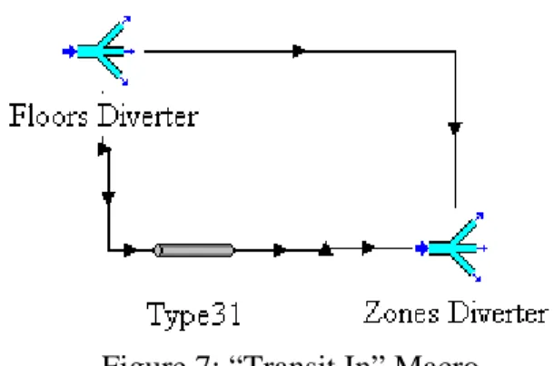
It represents the aeraulic network from AHU to the different zones. The “floors diverter” shown on figure 7 divides the airflows by 4, implying the hypothesis that the 4 floors behave all in the same way that the simulated one. The TRNSYS types used are similar to the previous macro.

(8)

8th International Conference on System Simulation in Buildings, Liege, December 13-15, 2010 Figure 7: “Transit In” Macro

4. SIMULATION OF THE EXISTING PRIMARY SYSTEM

The actual primary system consists of 3 classical (without condensation) gas boilers in cascade (318 kW each) for the heating water production. In TRNSYS, the 3 boilers have been considered as one 954 kW boiler. The chilled water is produced by an air-condenser heat pump (245 kW) equipped with 4 screw compressors. Both water networks are completely separated (see figure 8).

Figure 8: actual primary system

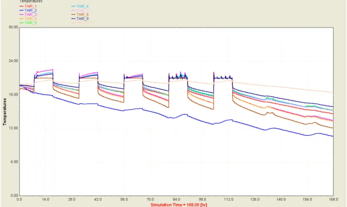
Even if the TRNSYS simulation for this first system is complete, some parameters are missing due to lack of as-built information. Realistic data has been used when necessary (details for the hydraulic network for example). Figure 9 shows a snapshot of the results obtained for the simulation of the first week of the year with the reference system. This graph shows the evolution of the air temperatures in the zones. One can notice that the 21°C set point is quite well respected during working hours. The energy consumption results (final energy) are listed in the table 1.

(9)

8th International Conference on System Simulation in Buildings, Liege, December 13-15, 2010 Figure 9: TRNSYS simulation (first week)

Table 1: results reference system

The first column indicates that the heating system has a rather good efficiency of almost 90%, taking into account all losses (regulation, distribution losses, exchangers’ efficiency…). On the other hand, the cooling system has an efficiency higher than unity. This results from the fact that the building demand was calculated for a perfect cooling system, able to reach 23°C in each zone at every time step. In reality, the system can reach its limits depending on the conditions in each zone. Sometimes, a cooling demand cannot be fulfilled and the energy produced is thus lower than the demand.

(10)

5. SIMULATION OF REVERSIBLE SYSTEM (AIR COUPLED)

The air coupled reversible system is based on AHPSAT model 1, which is composed of a reversible heat pump which is able to produce either cooling or heating water. However, both productions cannot be simultaneous and the priority is given to cooling capabilities. That’s why an auxiliary boiler is needed, for the cases when heating and cooling demands occur at the same time, or when the heat pump heating capacity is not sufficient. The sizing of the heat pump is made according to cooling demands, and the cooling capacity is thus the same as the previous case: 245 kW. The total power of the boiler is 954 kW.

Figure 8: reversible heat pump primary system

Table 2: results air coupled reversible system

The results of the simulation are listed in table 2. They are very similar to the first system. However it has to be noticed that the secondary system needs to be somehow adapted to the new primary system. Indeed, the heat exchangers have to deal with far lower temperatures in heating mode (≈ 45°C instead of ≈ 80°C). In these simulations, the heating coils (pre-heating and post-heating) have been designed to adequately transmit the energy to the air stream. Thus, they have to be oversized compared to the first case. The financial impact of such a change should be carefully studied in case of a retrofit of the building.

(11)

6. SIMULATION OF REVERSIBLE SYSTEM (GROUND COUPLED)

Figure 9: ground heat exchanger and reversible heat pump system

This system (model 5 in AHPSAT) is based on a reversible water to water heat pump of which heat/cold sink is a vertical ground heat exchanger (see figure 9). As for the previous system, the device is not able to supply heat and cold at the same time, and the priority is given to cold. In case of simultaneous demands, the heating is achieved thanks to an auxiliary gas boiler, also used when the heating demand is too high to be fulfilled by the heat pump alone. The capacities of the heat pump and boiler are respectively 245 kW and 954 kW.

Table 3: results ground coupled reversible system

The results of this last simulation are listed in table 3. The system seems to behave exactly as the previous one. Here, the high cost of the ground heat exchanger should be kept in mind in comparison with the air coupled system.

(12)

7. ANALYSIS & CONCLUSION

Model 0 Model 1 Model 5

Heating efficiency 89% 91% 91%

Cooling efficiency 148% 148% 148%

Table 4: efficiency summary

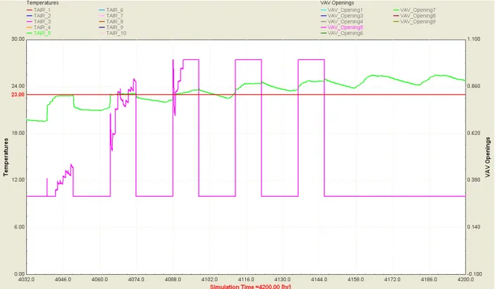
If the results of the 3 systems are compared (table 4), one can notice that the system heating efficiency is quite stable around 90% for the 3 models. On the other hand, the cooling efficiency is higher than unity. As discussed sooner, this last fact can be explained if one takes a look at the indoor conditions (see figure 10).

Indeed, in summer, the temperature in the zones can rise higher than 23°C, even if the corresponding VAV is open at 100%. As the primary system is correctly sized, this comes from secondary system limitations (regulation incompatibility, insufficient airflow…). As a result, the primary system produces less than the actual demand, and the apparent efficiency is higher than one. To tackle this issue, an increase in the ventilation rates or a decrease in the GP2 pulsed air temperature would be two options.

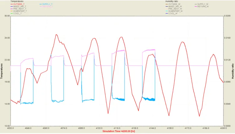
A plot of some AHU important temperatures is displayed on figure 11. The 14°C set point temperature is quite well respected during this summer week. Figure 12 shows the input and output temperatures of the heat pump for the same week. Here again, one can notice that the 7°C set point is achieved.

(13)

8th International Conference on System Simulation in Buildings, Liege, December 13-15, 2010 Figure 11: AHU supply, return and outside temperatures during one summer week

(14)

The results obtained can be converted into primary energy consumptions and compared to HPSAT figures, scaled to match the TRNSYS simulation configuration. The primary energy factors used are 3,31 and 1,35 for respectively electricity and gas. The primary energy consumption is composed of the gas needed for the boiler and the electricity needed for chiller. Circulation pumps, fans, appliances consumptions are not taken into account.

Figure 13 shows such a comparison. The graph clearly indicates that the gas consumption for the reference model is predominant. On the contrary the electricity represents the biggest part of the reversible systems consumptions. This means that the demand profiles of this building are adequate for reversibility, so that the heat pump is able to replace the boiler in many cases. The TRNSYS consumption results are logically higher than their corresponding results in AHPSAT, because they take into account the secondary system. This difference can be partially explained by the real indoor conditions reached, as discussed before, and by the differences in seasonal COP and EER reached (see table 5). This table seems to indicate that the hypothesis made about the heat pump performances in AHPSAT were too optimistic. The characteristics chosen in TRNSYS look more realistic. Another interesting fact is that the reversible heat pump performances are always higher in cooling mode than in heating mode, showing the lack of maturity of these devices in the domain.

(15)

Model 0 Model 1 Model 5

AHPSAT TRNSYS AHPSAT TRNSYS AHPSAT TRNSYS

COP / / 2,82 2,50 4,25 2,73

EER 5,05 2,95 4,80 2,95 5,66 4,56

Table 5: heat pump performances

For both simulations programs, the primary energy consumption of the reversible system is lower than the classical system (-16% in AHPSAT, -13% in TRNSYS). The primary energy consumption of the ground coupled system is the lowest (-36% in AHPSAT, -25% in TRNSYS).

AHPSAT TRNSYS

Reference model 100 100

Air coupled reversible 84,19 87,04

Ground couple reversible 63,86 74,96 Table 6: total primary energy consumption (ref system = 100)

The table 6 summarizes the results. The dynamic simulation of the whole system confirms the trend foreseen by AHPSAT: from an environmental point of view, the reversibility of the heat pump leads to primary energy savings, up to 25 % for a ground coupled system. However, this interesting result should be balanced with the economical impact of the installation of such a system (in a new construction and even more in a retrofit project).

(16)

8. REFERENCES

FABRY, B., BERTAGNOLIO, S., ANDRE, Ph., 2009. Performance evaluation of heat pump systems

in an office building, IEA-ECBCS Annex 48.

FABRY, B., DOLISY, V., BERTAGNIOLO, S., ANDRE, Ph., 2010. Detailed simulation of the

performance of heat pump systems in an office building, IEA-ECBCS Annex 48.

BELLIGOI, J., 2010. Audit énergétique d’un bâtiment de bureaux : proposition de stratégies de

rénovation. Mémoire de fin d’études, ULg.

SOCCAL, B., 2009. Performance Assessment Of Heat Pump Systems In Non-residential Buildings By

Means Of Dedicated Simulation Models. Mémoire de fin d’études, Ulg.

BERTAGNOLIO, S., GENDEBIEN, S., SOCCAL, B., STABAT, P., 2010. IEA48 Simulation Tools :

Reference Book, IEA-ECBCS Annex 48.

BERTAGNOLIO, S. et al., 2010, Simulation Based Assessment of Heat Pumping Potential in

Non-Residential Buildings – Part 1: Modeling, 10th REHVA World Congress - Clima 2010, Turkey.

BERTAGNOLIO, S.et al., 2010, Simulation Based Assessment of Heat Pumping Potential in

Non-Residential Buildings – Part 2: Parametric study, 10th REHVA World Congress - Clima 2010,

Turkey.

FABRY, B. et al., 2010, Simulation Based Assessment of Heat Pumping Potential in Non-Residential

Buildings – Part 3: Application to a typical office building in Belgium, 10th REHVA World Congress