O
pen
A
rchive
T
OULOUSE
A
rchive
O
uverte (
OATAO
)
OATAO is an open access repository that collects the work of Toulouse researchers and
makes it freely available over the web where possible.
This is an author-deposited version published in :
http://oatao.univ-toulouse.fr/
Eprints ID : 12778
Official URL: http://dx.doi.org/10.2991/eusflat.2013.4
To cite this version :
Dubois, Didier and Fargier, Hélène and Guyonnet,
Dominique Data Reconciliation under Fuzzy Constraints in Material Flow
Analysis. (2013) In: 8th European Society For Fuzzy Logic And Technology
Conference (EUSFLAT 2013), 11 September 2013 - 13 September 2013
(Milan, Italy).
Any correspondance concerning this service should be sent to the repository
administrator: [email protected]
Data Reconciliation under Fuzzy Constraints in
Material Flow Analysis
Didier Dubois
1, Hélène Fargier
1Dominique Guyonnet
21IRIT, CNRS & Université de Toulouse, France 2BRGM-ENAG, Orléans, France
Abstract
Data reconciliation consists in modifying noisy or unreliable data in order to make them consistent with a mathematical model (herein a material flow network). The conventional approach relies on least squares minimization. Here we show that the setting of fuzzy sets provides a generalized ap-proach that is more flexible and less dependent on oftentimes debatable probabilistic justifications. Moreover the proposed setting also encompasses constraint-based formulations using intervals.
Keywords: Material flow analysis, data reconcilia-tion, least squares, fuzzy constraints
1. Introduction
Material flow analysis consists in calculating the quantities of a certain product transiting a network of local entities referred to as processes, considering input and output flows and including the presence of material stocks. The unknowns to be determined are the values of the flows and stocks. The basic principle that provides constraints on the flows is that what goes into a process must come out, up to the variations of stock. Flows and stocks must be balanced, through a set of linear equations. The mass-balance equation relative to a process with n flows in, k flows out and a stock level s is written:
n Ø i=1 INi= k Ø j=1 OU Tj+ ∆s (1)
where ∆s is the amount of stock variation (positive ifqk
j=1OU Tj<qni=1INiand negative otherwise).
Such flow balancing equations in a process net-work define a linear system of the form Ayt= B, y
being the vector of N flows and stock variations. In order to evaluate balanced flows and stocks, data is collected regarding the material flow transiting the network and missing flow or stock variation val-ues are calculated. But this task may face several difficulties:
• There may not be sufficient information to de-termine all the missing flows or stock varia-tions.
• There may be on the contrary too much in-formation available and the system of balance equations may not have any solution.
• The available information is often not suffi-ciently reliable and precise.
In this paper we address the second and third cases. If the data are in conflict with the mass-balance equations, it may be because they are erroneous and should be corrected: this is the problem of data rec-onciliation, a well-known problem in statistics ever since its origins. As early as the end of the XVII-Ith century, this question was addressed using the method of least-squares. It still is the case today, but the justification is statistical and usually based on the Central Limit Theorem and the principle of maximum likelihood. In this paper, we examine the limitations of this approach and propose a prelimi-nary discussion on alternative approaches that take into account more explicitly data uncertainty, us-ing intervals or fuzzy intervals. Followus-ing the latter approaches, the problem can then be solved using crisp or fuzzy linear programming. We outline a general framework based on fuzzy intervals, under-stood as flexible constraints, that encompasses the least-squares method.
2. Data reconciliation
Data reconciliation consists in modifying measured or estimated quantities in order to balance the mass flows in a given network. The vector of flows y is subdivided into two sub-vectors x and u, i.e., k in-formed quantities xi and N − k totally unknown
quantities uj, to be determined. We denote by ˆx
the vector of available measurements ˆxi. In general,
the system A(xu)t = B has no solution such that
x = ˆx. This absence of solution is assumed to be
due to measurement errors or information defaults. The problem to be solved is to modify x, while re-maining as close as possible to ˆx, such that the mass
balance equations Ayt= B, with y = (xu), are
sat-isfied.
2.1. The least-squares approach
The traditional approach to data reconciliation [16] considers that data come from measurements, and measurement errors follow a Gaussian distribution with zero average and a diagonal covariance matrix. The precision of each measurement ˆxi, understood
as a mean value, is characterized by its standard deviation σi. Data reconciliation becomes a
prob-lem of optimization under linear constraints. In the simplest case (assuming no u):
Find x minimizing k Ø i=1 wi(xi− ˆxi)2 such that Axt= b
It is the method of weighted least-squares used in many data reconciliation packages such as STAN [2]. The solution is known to be of the form [16]:
x∗= ˆx − W−1At(AW−1At)−1A(ˆx − b),
where W is a diagonal matrix containing terms 1/wi. Weights are often of the form wi= (σi)−2.
Such packages sometimes also reconcile variances as explained in [16]. It assumes that the vector of estimated values ˆx has a multivariate normal
distri-bution characterized, by a covariance matrix C gen-eralizing W , whose diagonal contains the variances
σ2
i. The balance flows being linear, the reconciled
values x∗ depend to the estimated values via a
lin-ear transformation, say x∗= B ˆx hence also have a
normal distribution. The covariance matrix of x∗is
then of the form C∗= BCBt.
2.2. Limitations of the approach
The method of least-squares is often justified based on the principle of maximum likelihood, applied to normal distributions, in turn justified by the Central Limit Theorem (CLT). If pi is the probability
den-sity function associated with error ǫi= xi− ˆxi, the
maximum likelihood is calculated on the function
L(x) =rk
i=1pi(xi− ˆxi). If the pi’s are normal with
average 0 and standard deviation σi, then pi(xi−ˆxi)
is proportional to e−
(xi−ˆxi)2 σ2
i . As a consequence, the
maximum of L(x) coincides with the solution to the least squares method. The Gaussian assump-tion seems to be made because of the popularity of Gauss law (that computes an approximation of the standard deviation of a function f (x1, . . . xk) in the
vicinity of a measurement point based on the linear part of its Taylor expansion). The universal char-acter of this approach, albeit reasonable in certain situations, is nevertheless dubious:
• It is not consistent with the history of statis-tics [18]. The least-squares method, developed by Legendre (1805) and Gauss (end of XVII-Ith century), was discovered prior to the CLT, as is the Gauss function. Invented precisely to solve a problem of data reconciliation in astron-omy, the least squares method sounded natural since it was in accordance with the Euclidean distance. Moreover, it led to solutions that could be calculated analytically and it could justify the use of the average in the estimation of quantities based on several independent mea-sures. The normal law was discovered by Gauss as the only error function that was compatible
with the average estimator. However, CLT is a mathematical result obtained independently by Laplace, who later on made the connection between his mathematical result and the least squares method.
• The CLT presupposes a statistical process with a finite average E and standard deviation σ. In this case, the average of n random variables vi
has standard deviation σ/√n and the
distribu-tion of the average qn
i=1√vi−nE
n is
asymptoti-cally Gaussian as n increases. The fundamen-tal hypothesis behind the normal distribution is the existence of a finite σ. In practice, this implies that for N observations aiof v, the
em-pirical variance msd = 2 q
i<j(ai−aj)
2
N(N −1) remains
bounded as N increases, which is neither al-ways true nor easily verifiable.
• The Gaussian hypothesis is only valid in the case of an unbounded random variable. If
vi is positive or bounded, assuming that the
quantity En =
qn i=1vi
n assymptotically follows
a normal distribution with standard deviation
σ/√n is an approximation that may be useful
in practice but does not constitute a general principle.
Based on the remarks above, it is natural to look for alternative methods for reconciling data that do not come from a statistical measurement process. A first alternative consists in representing error-tainted data by means of intervals and checking the compatibility between these intervals.
3. Interval reconciliation
In practice, information on mass flows is seldom precise: the data-gathering process often relies on subjective expert knowledge or on scarce measure-ments published in various documeasure-ments that more-over might be obsolete. Each flow value provided by a source can be more safely represented by an in-terval ˆXi, which in a first stance, can be considered
as encompassing the actual flow value: of course, the less precise the available information, the wider the interval. Missing values ui can also be taken
into account: we then select as its attached interval the domain of possible values of the corresponding parameter (for example, the unknown grade of an ore extracted from a mine and sent to the treat-ment plant can, by default, be represented by the interval [0 ,100]%). In the least-squares approach to data reconciliation, we use weights to reflect the as-sumed variance of a Gaussian phenomenon; if such information on variances σ2
i are available, we can
set ˆXi = [ˆxi− 3σi, ˆxi+ 3σi], as the distribution of
xi is often assumed to be Gaussian. Thus each of
the N variables yi of the vector y = xu is delimited
a priori by an interval ˆYi.
us to consider the reconciliation as a problem of constraint satisfaction; the mass balance equations must be satisfied for flux and stock values that lie within the specified intervals - or, to be more pre-cise, we can restrain these intervals to the sole values that are compatible with the balancing model given the possible values of other variables. Formally, the reconciliation problem can be expressed as follows: For each i = 1, . . . N , find the smallest and largest values for yi, such that :
Ayt= B
yi∈ ˆYi, i = 1, . . . , N
The calculation of consistent minimum and max-imum values of yi is sufficient: since all the
equa-tions are linear, we can show that if there exists two flow vectors y and y′, each being a solution to the
above system of equations, then any vector v lying between y and y′componentwise is a solution of the
system of equations Ayt= B. The problem can of
course be solved using linear programming. Due to the linearity of the constraints, it may also be solved by methods based on interval propagation. For each variable yi, equation j of the system Ayt=
B can be expressed as yi = q kÓ=ibj− ajkyk aji , i = 1, . . . , N.
We can then project this constraint on yi and find
the possible values of yi consistent with it. Due
to the m linear constraints, the values of yi can be
restricted to lie in the interval:
Yi= ˆYi∩ (∩j=1...,m q kÓ=ibj− ajkYˆk aji ), where q kÓ=ibj−ajk ˆ Yk
aji is calculated according to the
laws of interval arithmetic [12]; if the new interval of possible values of yi is more precise (Yi⊂ ˆYi), it
is in turn propagated to the other variables. This procedure, known as “arc consistency”, is iterated until intervals are stabilized; it converges within a finite number of steps to a unique set of intervals [13] (for additional details on interval propagation techniques, see [1, 11]). Note that contrary to the statistical approach, here the model constraints and the imprecise data are handled on a par.
4. Modeling data using fuzzy intervals
In the framework of measurement problems, Mau-ris [14] has suggested that in the case of competing error functions (empirical probability distributions
pi, i = 1 . . . k), one may refrain from choosing one
of them and consider a family of probabilities P in-stead, to represent our knowledge about x, where
pi ∈ P, ∀i. In general such a representation can
be extremely complex. For instance, P should be convex, typically the convex hull of {pi, i = 1 . . . k}.
However a very simple and convenient representa-tion is via possibility distriburepresenta-tions having the shape of a fuzzy interval [4].
A possibility distribution is a mapping π : R → [0, 1] such that π(r∗) = 1 for some r∗∈ R. It
repre-sents the current information on a quantity x. The idea is that π(r) = 0 if and only if x = r is impos-sible, while π(r) = 1 if x = r is a totally normal, expected, unsurprizing value. One rationale for this framework is that the set Iα= {r, π(r) ≥ α} (α-cut)
contains x with level of confidence 1 − α, that can be interpreted as a lower probability bound. In par-ticular, it is sure that x ∈ {r, π(r) > 0} = S(π), the support of the possibility distribution.
A fuzzy interval is a possibility distribution whose
α-cuts Iα are closed intervals. They form a nested
family of intervals containing the core C(π) = {r, π(r) ≥ α} = 1 and contained in the support. The simplest representation of a fuzzy interval is a trapezoid defined by the core and the support. Note that this format is very convenient to gather information from experts in the form of confidence intervals.
Given a possibility distribution π, the degree of possibility of an event A is Π(A) = supr∈Aπ(r).
The degree of certainty of event A is N (A) = 1 − Π(Ac), where Ac is the complement of A. A
possibility distribution can be viewed as encoding a convex probability family P(π) = {P, P (A) ≥
N (A), ∀A measurable} (see [4] for references).
Functions Π and N can be shown to compute exact probability bounds in the sense that
Π(A) = sup
P∈P(π)
P (A) and N (A) = inf
P∈P(π)P (A).
When several error functions are possible, one may choose to represent them by a possibility distri-bution that encompasses them. This is the idea de-veloped by Mauris [14]. Probabilistic inequalities is one example. For instance, knowing the mean value and the standard deviation of a random quantity, Chebyshev inequality gives a possibility distribution that encompasses all probability distributions hav-ing such characteristics [7]. Gauss inequality also provides such possibility distributions encompass-ing probability distributions with fixed mode and standard deviation (see [15]). It yields a triangular (bounded) fuzzy interval if probability distributions have bounded support. Hence a possibility distri-bution may account for incomplete statistical data. Conversely, if an expert provides a probability distribution that represents subjective belief, it is possible to reconstruct a possibility distribution that fits the Laplace principle of indifference. When the available knowledge is an interval [a, b], and the expert is forced to propose a probability distribu-tion, the most likely proposal is a uniform distri-bution over [a, b] due to symmetry. If the available knowledge is a possibility distribution π, this sym-metry argument leads to replace π by a probability
distribution constructed by (i) picking at random a threshold α ∈ [0, 1] and (ii) a number at random in the α-cut Iα of π. One may argue that we should
bet on the basis of this probability function in the absence of any other information. Conversely, a subjective probability provided by an expert can be represented by the (unique) possibility distribution that would yield this probability distribution using this two-stepped random Monte-Carlo process [10]. In summary, fuzzy intervals, and specifically tri-angular or trapezoidal possibility distributions, may account for various kinds of uncertain information.
5. Fuzzy interval reconciliation
The interval approach does not yield the same type of answer as the least-squares method because it provides only intervals rather than precise values. Such intervals can be compared to reconciled vari-ances provided by current software for MFA and data reconciliation like STAN [2]. A natural way to obtain both reconciled values and intervals is to tolerate a certain level of flexibility on the flow esti-mates using the notion of fuzzy interval: the more-or-less possible values of each flow or stock yi will
be limited by a fuzzy interval ˜Yi. For some of these
quantities, these constraints will be satisfied to a certain degree, rather than simply either satisfied or violated. The problem of searching for a possible solution then becomes an optimization problem - we seek an optimal position within all the (fuzzy) inter-vals of possible values. If no solution provides entire satisfaction for all intervals, some will be relaxed if necessary [5].
5.1. A general framework
In this approach, the linear equations describing the material flow for each process are considered as in-tegrity constraints that must necessarily be satis-fied, but the information relative to possible values of each flow or stock quantity yiis represented, not
as a strict interval ˆYi but as a fuzzy interval ˜Yi,
interpreted as a possibility distribution πi. This
interval may still coincide with the domain of the quantity, in the case of total ignorance.
An assignment y for all yiis possible, provided it
satisfies all the constraints. In other words, the de-gree of plausibility of an assignment y = xu can be obtained by a conjunctive aggregation of the local satisfaction degrees. Namely it is ⋆N
i=1π(yi) if y
sat-isfies the integrity constraints, and 0 otherwise - the operation ⋆ being associative, commutative and in-creasing on [0, 1] (a t-norm). We may then calculate the most plausible reconciled vectors and the asso-ciated degree of possibility by solving the following problem:
Find the values y = xu that maximize:
π⋆(y) = ⋆Ni=1πi(yi) such that Ayt= B
Rather than providing the user with one amongst several optimal solutions, it is often more informa-tive to have reconciled flows in the form of fuzzy intervals obtained by projection on the domain of each yi:
max
y s.t. yi=v and Ayt=B⋆
N
j=1πj(yj)
The operator models the fact that the yi must be
placed as close as possible to the cores of the fuzzy intervals - to their center if we use triangular (or trapezoidal) representations. In the case of “classi-cal” intervals, i.e. when degrees of membership to the ˜Yi’s are 0 or 1, the ⋆ operator performs a simple
conjunction and we come back to the formulation of Section 3. The cases ⋆ = min and ⋆ = product con-stitute two basic modeling choices. We may also use the Łukasiewicz t-norm : max(0, a + b − 1), which eliminates as impossible some vectors y that have albeit positive but too low scores. The first opera-tor, the minimum, nevertheless presents advantages from a computation viewpoint: it allows the use of tools from linear programming or interval propaga-tion.
5.2. The max-min approach
The optimization problem to be solved takes the form:
Find y∗ that maximizes
πmin(y) =
N
min
i=1πi(yi) where Ay
t= B
with Ayt = B. Let α∗ = minN
i=1πi(yi∗) where y∗
is an optimal solution. This implies that we cannot aim at a plausibility value α > α∗, since there will
be no simultaneous choice of the yi in the α-cuts
of ˜Yi that will form a consistent vector in the sense
of the network defined by Ayt= B, whereas there
exists at least one consistent assignment of flows at the level α∗. Note that there may exist several
solutions that allow a level of satisfaction α∗.
Once α∗ is known, we can assign to each flow an
interval of optimal values ( ˜Yi)α∗ = {yi : πi(yi) ≥ α∗} by solving for each y
i the following interval
reconciliation problem: Find the minimum (resp. maximum) values of yi such that Ayt= B and:
πj(yj) ≥ α∗, j = 1, . . . , N.
The fuzzy reconciliation problem fails if α∗ = 0.
The optimal supports of the optimal fuzzy intervals containing the yi’s can be obtained if we use the
supports of the ˜Yi in the procedure of the previous
section. This program contains on the one hand the mass flow model Ayt= B which, as seen previously,
is linear, and then we force the yi to belong to the
supports [si, si], i = 1, . . . N of the fuzzy intervals
˜
5.3. Resolution methods
From a technical standpoint, the fuzzy interval rec-onciliation problem can be solved using three alter-native approaches:
Using a fuzzy interval propagation algorithm
As in the crisp case, fuzzy intervals of possible val-ues ˜Yi can be improved by projecting the fuzzy
do-mains of other variables over the domain of yi via
the balancing equations: ˜ Yi′= ˜Yi∩ (∩j=1...,m q kÓ=ibj− ajkY˜k aji ), where q kÓ=ibj−ajk ˜ Yk
aji is a fuzzy interval ˜Aj that
can be easily obtained by means of fuzzy inter-val arithmetics [8] since equations are linear. Note that ˜Yi∩ (∩j=1...,mA˜j) has possibility distribution
π′
i= min(πi, minj=1...,mπA˜j).
The propagation algorithm iterates these up-dates by propagating the new fuzzy intervals on all the neighboring yi’s, until their domains no longer
evolve. This procedure presupposes efficient fuzzy interval representation schemes must be used. Typ-ically we should use piecewise linear fuzzy intervals [17] including subnormalized ones. Eventually, op-timal (maximally precise) fuzzy intervals ˜Yi∗are
ob-tained as resulting fuzzy domains of the reconciled flows. These fuzzy domains may be subnormalized: at least one of them has height hi= supyiπ
∗
i(yi) =
α∗ that may be less than 1 and may contain a
sin-gle value. However the heights hj of other
opti-mal fuzzy intervals may be greater that α∗. Their
hj-cuts contain the optimal values yi∗. However,
this method will only provide the fuzzy intervals with possibility distributions min(πi, α∗) since fuzzy
arithmetic methods applied to fuzzy intervals of var-ious heights only preserve the least height [8].
Using α-cuts In order to take advantage of the
calculation power of modern linear programming packages, a simple solution is to proceed by di-chotomy on the α-cuts of the fuzzy intervals : once each ˜Yi is cut at a given level α, we obtain a
sys-tem of equations as in Section 3, replacing ˆYi by the
interval ( ˜Yi)α; this system can therefore be solved
by calling an efficient linear programming solver. If the solver finds a solution, the level α is increased; if not, i.e., if it detects an inconsistency in the system of equations, the value α is decreased, etc. until the maximum value α∗is obtained with sufficient
preci-sion, along with the corresponding intervals ( ˜Yi)α∗.
Using fuzzy linear programming When the fuzzy intervals are triangular or trapezoidal (or even homothetic, as in the case of L-R fuzzy numbers), it is possible to write a (classical) linear program in order to obtain the value of α∗, then obtain the
optimal ranges ( ˜Yi)α∗’s for the reconciled flows. It
is necessary to model the fact that the global de-gree of plausibility of the optimal reconciled val-ues is the least among the local degrees of possi-bility, i.e., we should maximize a value less than all the πi(yi), hence we should write N constraints
α ≤ πi(yi), i = 1, . . . , N . When the original fuzzy
intervals are triangular with core ˆyi, each constraint
is written in the form of two linear inequalities, one for each side of the fuzzy intervals. All these equa-tions being linear, we can then use a linear solver to maximize the value α such that:
Ayt= B
si≤ yi≤ si, i = 1, . . . , N
α(ˆyi− si) ≤ yi− si, i = 1, . . . , N
α(si− ˆyi) ≤ si− yi, i = 1, . . . , N
The same type of modeling yields the inf and sup limits of the α∗-cuts for the reconciled intervals ˜Y∗
i
(maximizing and minimizing yi, letting α = α∗ in
the constraints above). By virtue of the linearity of the system of equations and of the membership functions, we can reconstruct the reconciled ˜Y∗
i up
to possibility level α∗ by linear interpolation
be-tween the cores and the optimal supports obtained by deleting the third and fourth constraints in the above program (although strictly speaking the rec-onciled fuzzy intervals might only be piecewise lin-ear).
It is possible (and recommended) to iterate the above procedure and refine the optimal intervals ( ˜Yi)α∗ by instanciating the quantities yi such that
( ˜Yi)α∗ reduces to a singleton {y∗
i} as described in
[6], leaving other variables in their optimal α∗-cuts.
Namely, let V1 = {i : ( ˜Yi)α∗ = y∗
i}. We can solve
the problem of maximizing the value α such that
Ayt= B si≤ yi≤ si, i Ó∈ V1 yi= yi∗, i ∈ V1 α(ˆyi− si) ≤ yi− si, i Ó∈ V1 α(si− ˆyi) ≤ si− yi, i Ó∈ V1 α ≥ α∗
Then we get an optimal value α∗
1> α∗, and we can
look for the optimal ranges ( ˜Yi)α∗
1, i ∈ V1 some of
which again reduce to singletons. So, at this second step we have instanciated a set V2⊃ V1of variables.
We can iterate this procedure until all variables are instanciated, at various levels of optimal pos-sibilities. Eventually, it delivers precise reconciled values along with possibility distributions around them. These values are Pareto-optimal in the sense of the vector-maximisation of the vectors (π1(y1), . . . πN(yN)).
Among the three approaches, the latter based on fuzzy linear programming looks like the most con-venient one.
y1 y2 y3 y4
Least squares method
Original data 24 ± 2 16 ± 3 15 ± 4 22 ± 5
Reconciliated values 23, 8 15, 5 15, 9 23, 4
Reconciliated fuzzy intervals
Triangular fuzzy intervals (22, 24, 26) (13, 16, 19) (11, 15, 19) (17, 22, 27)
α∗: 11 14
Reconciliated cores 23 + 4/7 15 + 5/14 15 + 6/7 23 + 1/14 Reconciliated supports [22, 26] [13, 19] [11, 19] [17, 27]
Table 1: Reconciliated flows for Example 1
6. Some examples
We present simple examples in order to compare the statistical and fuzzy approaches
6.1. One-process case
We consider the example illustrated in Figure 1, which is composed of four flows (y1, y2, y3, y4) and
one process (P1). Flows y1 and y2 enter the
pro-cess, while y3 and y4exit the process. There are no
stocks. In this example we have symmetric trian-gular fuzzy intervals ˜Y1= 24 ± 2, ˜Y2= 16 ± 3, ˜Y3=
15 ± 4, ˜Y4= 22 ± 5. In the least-squares method, we
interpret the half-length of the interval as a stan-dard deviation.
Figure 1: Example 1
With the fuzzy interval approach, the calculation of
α∗ using linear programming is obtained by solving
the following linear problem: Maximize α such that:
y1+ y2= y3+ y4 22 ≤ y1≤ 26 α · (26 − 24) ≤ 26 − y1 α · (24 − 22) ≤ y1− 22 13 ≤ y2≤ 19 α · (19 − 16) ≤ 19 − y2 α · (16 − 13) ≤ y2− 13 11 ≤ y3≤ 19 α · (19 − 15) ≤ 19 − y3 α · (15 − 11) ≤ y3− 11 17 ≤ y4≤ 27 α · (27 − 22) ≤ 27 − y4 α · (22 − 17) ≤ y4− 17 Figure 2: Example 2
The results obtained using the two methods (least-squares and fuzzy interval reconciliation) are provided in Table 1. We note that the alpha-cuts of the fuzzy intervals at level α∗ after propagation
are singletons and that the maximum deviation be-tween the initial and reconciled values is smaller in the case of the fuzzy method than with the least-squares method.
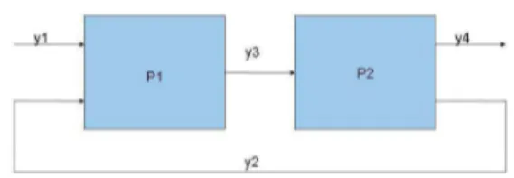
6.2. Two-process example
We consider the example in Figure 2, composed of four flows (y1, y2, y3, y4) and two processes (P1 and
P2). Flows y1 and y2 both enter process P1; y3
exits P1 to enter P2, two flows exit P2: y4 and y2,
while the latter is recycled into P1. In this example ˜
Y1= 20 ± 3, ˜Y2= 10 ± 2, ˜Y3∈ 20 ± 4, ˜Y4= 16 ± 3.
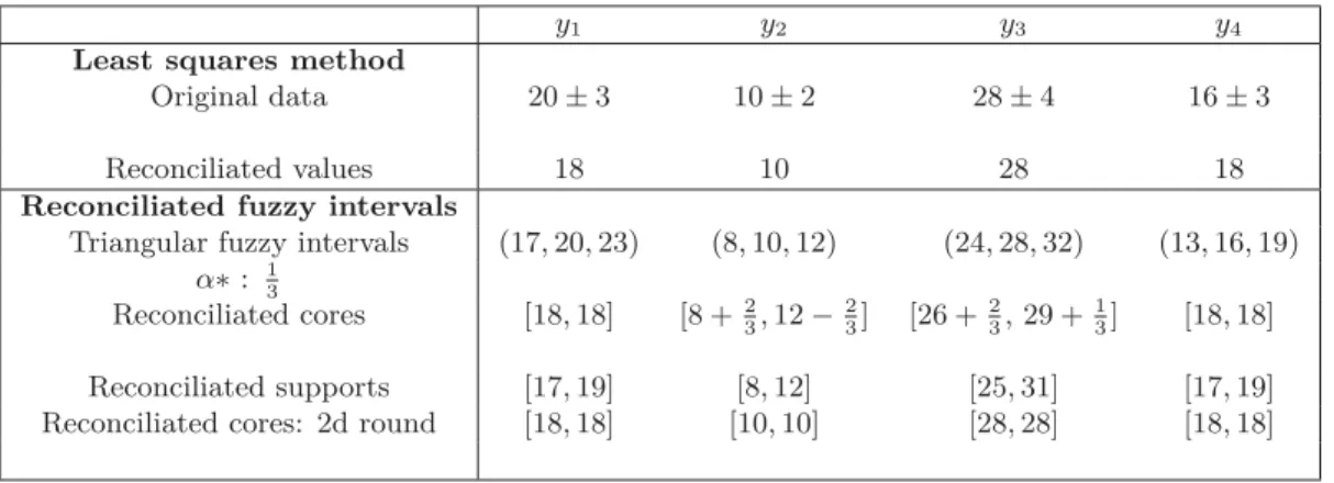
For the approach using fuzzy intervals, the calcu-lation of α∗ by linear programming is obtained by
solving a system of equations similar to that of the previous case. We obtain α∗ = 1/3. We can also
obtain this value by calculating the height of ˜Y1∩ ˜Y4.
Indicated in Table 2 are the cuts at level 1/3 and the supports of the reconciled fuzzy intervals. We note that reconciled values obtained by least-squares are at the center of the supports of the reconciled inter-vals obtained using the fuzzy interval method.
However, it is possible to refine the remaining in-tervals. If we retain the information y∗
1 = y∗4 = 18
and run the fuzzy interval propagation procedure again, we verify that the intersection ˜Y2∩ ( ˜Y3− 18)
can also fix y3 = 28 considering ˜Y3 ∩ ( ˜Y2 + 18).
We can therefore verify that π1(18) = π4(18) =
1/3, π2(10) = π3(28) = 1 and therefore that the
least-squares solution coincides in this particular ex-ample with the Pareto-optimal solution of the fuzzy data reconciliation problem. The former example shows that this is not always the case.
6.3. Comparing reconciled values: a generic example
Consider a single process with n inputs xi and a
single output x0 = qni=1xi. Suppose all
mea-sured inputs are ˆxi = a > 0 while ˆx0 = ka > 0.
One may argue that, assuming the xi’s have the
same variance 1, x0 has variance equal to n. It is
easy to obtain least squares estimates, minimizing qn
i=1(xi− a)2+(x0−a)
2
n under the balancing
con-straint. It is easy to find that xLS
0 = a(k+n)2 and
xLS i = a2+
ak
2n. Note that limn→∞xLSi = a/2 and in
fact a
2 < xLSi ≤ a(k+1)
2 . All reconciled flows linearly
increase to infinity if k increases.
In the fuzzy interval approach we can assume tri-angular membership functions : X˜i has mode a
and support [a − α, a + β], where the magnitudes of α, β depend on the available knowledge. Sup-pose that the relative error of the data is every-where the same so that ˆX0 has mode ka and
sup-port [k(a−α), k(a+β)]. The reconciled value for x0
is obtained as the value for which the intersection ˆ
X0∩ n ˜Xi has maximal positive possibility degree.
There are two cases
x∗ 0=
Inka(α+β)
nα+kβ if k ≤ n and k(a + β) > n(a − α)
nka(α+β)
kα+nβ if k ≥ n and k(a − α) < n(a + β).
It can be checked that the least squares solution is encompassed by the fuzzy interval approach. If
k ≤ n, x∗
0 = xLS0 if and only if α, β are chosen such
that nα = kβ > a(n−k)2 (the inequality makes the fuzzy reconciliation problem feasible). Likewise, if
n ≥ k, the condition is kα = nβ > a(n−k)2 .
Finally we check when x∗
0 is closer to the
esti-mated value ka than xLS
0 . For instance, if k ≤ n,
x∗
0 > ka and xLS0 > ka, and xLS0 > x∗0 > ka
pro-vided that kβ < nα.
7. A unified framework for least squares and fuzzy interval reconciliation
If we select the product for operation ⋆ in the gen-eral formulation of Section 5.1, the reconciliation problem boils down to maximizing the expression
π⊙(y) = rN
i=1πi(yi) under constraints Ayt = B.
If in addition we choose to use Gaussian shapes
πi(y) = e
−(yi−ˆσ2yi)2
i for the fuzzy intervals, it becomes
clear that this formulation brings us precisely back to the maximum likelihood expression L(x). There-fore the fuzzy interval approach defined in Section
5.1 captures the least-squares method as a special case, minimizing the distance to estimated values in the sense of the l2 norm.
With ⋆ = min and triangular fuzzy intervals ˜Yi
centered around measured values ˆyi, solving the
max-min fuzzy constraint problem, reduces to min-imizing the maximal weighted absolute deviation:
e∞(y) = max
i=1,...,N
|yi− ˆyi|
σi
,
using an l∞norm instead of the Euclidean l2norm.
Here σi is interpreted as the spread of the fuzzy
interval ˜Yi.
Similarly, choosing a ⋆ b = max(0, a + b − 1) un-der the same hypotheses comes down to minimizing a weighted sum of absolute errors, i.e., use the l1
norm: e1(y) = Ø i=1,...,N |yi− ˆyi| σi .
More generally recent works on penalty-based ag-gregation [3] may help us find an even more general setting for devising reconciliation methods in terms of general penalty schemes when deviating from the measured data flows.
8. Conclusion
In the context of the mass flow reconciliation prob-lem, we often deal with scarce data of various ori-gins, pertaining to different quantities, that we can hardly assume to be generated by a standard ran-dom process. It seems more natural to concentrate efforts on the choice of a distance (l1, l2, l∞, . . . ) for
minimizing the error rather than to invoke the CLT to justify the least-squares method. A fuzzy-set ap-proach to data reconciliation has been proposed. Its advantages are:
• Its general character: in a formal sense, it gen-eralizes the least-squares method without be-traying the principle of maximum likelihood. Indeed, it is well-known that a likelihood func-tion is a special case of a possibility distribufunc-tion [9] and we see clearly that the likelihood L(x) is a special case of π⋆(x), with ⋆ = product.
• Its clear conceptual framework, both for repre-senting uncertainty pervading the data (statis-tical or subjective) and for leaving the choice of the distance that enters the error function to the user. The reconciled ranges around the reconciled values are also more easy to inter-pret than the reconciled variances, as they re-sult from standard interval propagation. • The opportunity of solving the problem in the
max-min case, using standard methods and software.
However, our framework does not encompass the probabilistic method of variance reconciliation de-scribed in Section 2.1, since the latter views the nor-mal distribution on flow measurements as a data
y1 y2 y3 y4
Least squares method
Original data 20 ± 3 10 ± 2 28 ± 4 16 ± 3
Reconciliated values 18 10 28 18
Reconciliated fuzzy intervals
Triangular fuzzy intervals (17, 20, 23) (8, 10, 12) (24, 28, 32) (13, 16, 19)
α∗ : 1 3 Reconciliated cores [18, 18] [8 +2 3, 12 − 2 3] [26 + 2 3,29 + 1 3] [18, 18] Reconciliated supports [17, 19] [8, 12] [25, 31] [17, 19]
Reconciliated cores: 2d round [18, 18] [10, 10] [28, 28] [18, 18]
Table 2: Reconciliated flows For Example 2
generation process and not as an additional con-straint. In contrast one could consider reconciling variances as a data fusion problem.
Mind that minimizing a sum of absolute valued deviations (and to a lesser extent quadratic), runs the risk of making certain values of xi deviate
sig-nificantly from the data ˆxi, whereas the max-min
approach is designed to keep all of them as close as possible to the initial data. The latter approach seems to be more reasonable if the data come as single estimate from an expert or other sources for each quantity. This approach is currently being studied for analyzing the material flow of rare earth elements in the anthroposphere of the EU-27.
Acknowledgements This work is supported by the French National Research Agency (ANR), as part of Project ANR-11-ECOT-002 ASTER “Sys-temic Analysis of Rare Earths - flows and stocks”.
References
[1] F. Benhamou, L. Granvilliers, F. Goualard. In-terval Constraints: Results and Perspectives.
New Trends in Constraints, LNAI 1865, pages
1-16, Springer, 2000. 22nd European Symposium
on Computer Aided Process Engineering (I.D.
Lockart Bogle, M. Fairweather, Eds.), Elsevier 2012, 122-126
[2] P.H. Brunner and H. Rechberger (2004). Practi-cal Handbook of Material Flow Analysis. Lewis Publishers.
[3] T. Calvo, G. Beliakov Aggregation functions based on penalties, Fuzzy Sets and Systems, 161(10), 2010, 1420-1436.
[4] D. Dubois Possibility theory and statistical rea-soning Comput. Stat. & Data Anal., 51, 47-69, 2006
[5] D. Dubois, H. Fargier, H. Prade. Possibility the-ory in constraint satisfaction problems: Han-dling priority, preference and uncertainty.
Ap-plied Intelligence, 6, 287-309, 1996.
[6] D. Dubois, P. Fortemps. Computing improved optimal solutions to max-min flexible constraint
satisfaction problems. Eur. J. of Operation
Re-search, 118, 95-126, 1999.
[7] Dubois D. Foulloy L. Mauris G. Prade H. Probability-possibility transformations, trian-gular fuzzy sets, and probabilistic inequalities.
Reliable Computing. 2004. 10, 273-297
[8] D. Dubois, E. Kerre, R. Mesiar, H. Prade. Fuzzy interval analysis. In: Fundamentals of
Fuzzy Sets, Dubois, D. Prade, H., Eds: Kluwer, Boston, Mass, The Handbooks of Fuzzy Sets Se-ries, 483-581, 2000.
[9] D. Dubois, S. Moral, H. Prade. A semantics for possibility theory based on likelihoods. J. of
Math. Anal. Appl., 205, 359-380, 1997.
[10] D. Dubois, H. Prade, Philippe Smets: A def-inition of subjective possibility. Int. J. Approx.
Reasoning 48(2): 352-364 (2008)
[11] L. Granvilliers, F. Benhamou. Algorithm 852: RealPaver: an interval solver using constraint satisfaction techniques. ACM Trans. on
Mathe-matical Software32(1), 138-156, 2006.
[12] L. Jaulin, M. Kieffer, O. Didrit, E. Walter.
Ap-plied Interval Analysis, Springer, London, 2001. [13] O. Lhomme. Consistency Techniques for Nu-meric CSPs. Proc. Int. Joint Conf on Artificial
Intelligence(IJCAI 1993), pages 232-238. [14] G. Mauris: Expression of Measurement
Uncer-tainty in a Very Limited Knowledge Context: A Possibility Theory-Based Approach. IEEE T.
Instrum. and Meas.56(3): 731-735 (2007) [15] G. Mauris: Possibility distributions: A unified
representation of usual direct-probability-based parameter estimation methods, Int. J. of
Ap-prox. Reasoning, 52(9), 1232-1242 (2011). [16] S. Narasimhan, C. Jordache, Data
reconcili-ation and gross error detection: an intelligent use of process data, Gulf Publishing Company, Houston, 2000.
[17] H. Steyaert, F. Van Parys, R. Baekeland and E. Kerre. Implementation of piecewise linear fuzzy quantities, Int. J. Intelligent Systems, 10, 1049-1059, 1995.
[18] S. M. Stigler. The History of Statistics: The
Measurement of Uncertainty before 1900. Belk-nap Press/Harvard University Press, 1990.