Trois essais sur la persistance inflationniste et la dynamique cyclique : le rôle central des rigidités nominales et de la structure de production en boucle

TROIS ESSAIS SUR LA PERSISTANCE INFLATIO NISTE ET LA DYNA\1IQUE CYCLIQUE : LE RÔLE CENTRAL DES RIGIDITÉS NOMINALES ET DE LA STRUCTURE DE PRODUCTION EN BOUCLE

THÈSE PRÉSENTÉE

C0\1ME EXIGENCE PARTIELLE

DU DOCTORAT E ÉCONOMIQUE

PAR

SALAHEDDI E EL 0\1ARI

UNIVERSITÉ DU QUÉBEC

À MONTRÉAL

Service des bibliothèques

Avertissement

La diffusion de cette thèse se fait dans le respect des droits de son auteur, qui a signé le formulaire Autorisation de reproduire et de diffuser un travail de recherche de cycles supérieurs (SDU-522 - Rév.01-2006). Cette autorisation stipule que «conformément

à

l'article 11 du Règlement no 8 des études de cycles supérieurs, [l'auteur] concède à l'Université du Québec

à

Montréal une licence non exclusive d'utilisation et de publication de la totalité ou d'une partie importante de [son] travail de recherche pour des fins pédagogiques et non commerciales. Plus précisément, [rauteur] autorise l'Université du Québec

à Montréal

à

reproduire, diffuser, prêter, distribuer ou vendre des copies de [son] travail de recherche

à

des fins non commerciales sur quelque support que ce soit, y compris l'Internet. Cette licence et cette autorisation n'entraînent pas une renonciation de [la] part [de l'auteur] à [ses] droits moraux ni à [ses] droits de propriété intellectuelle. Sauf entente contraire, [l'auteur] conserve la liberté de diffuser et de commercialiser ou non ce travail dont [il] possède un exemplaire.»

Tout à bord, je tiens à remercier Dieu qui m'a donné la force et la santé pour achever mon doctorat. Ensuite, je voudrais remercier, Louis Phaneuf, mon directeur de thèse qui fut, au cours des six années qui viennent de s'écouler, bien plus qu'un directeur. Je crois même ne plus savoir pourquoi je dois le remercier tant il fut important, sans doute pour tout. Travailler sous sa direction est une école de rigueur et de curiosité scientifique, de disponibilité et d'enthousiasme. Enfin, de tout mon coeur, merci d'avoir toujours su insuffler l'envie d'apprendre et de m'avoir supporté financièrement et moralement durant mes études doctorales.

Je suis également reconnaissant à tous les professeurs qui m'ont enseigné au Dé-partement des sciences économiques de l'UQAM. Je ne saurai oublier mes amis à l'Uni -versité du Québec à Montréal dont en particulier Ajmi Ben Khalifa, Kamel Zeghba, Sêgnon AGUEY, Boubacar Diallo, ainsi que le personnel administratif du Département des sciences économiques de l'UQAM dont je cite en particulier Jasée Parenteau, Mar-tine Boisselle, Jacinthe Lalande, Julie Hudon, Francine Germain et Lorraine Brisson. Je tiens à remercier également mon collègue et mon ami Stéphane Demers pour son aide et son sou tien moral.

J'associe à ces pensées mes soeurs Asma, Safaa et Sanaa et mon frère Yassine. C'est à mes parents que je pense au moment où j'écris ces quelques lignes. Avec beaucoup d'Amour! Merci mes parents pour votre soutien inconditionnel et votre amour.

-

-TABLE DES MATIÈRES

REMERCIEMENTS 11

LISTE DES FIGURES . VI

LISTE DES TABLEAUX IX

RÉSUMÉ . . . x

I TRODUCTION 1

CHAPITRE I

THE MULTIPLIER FOR PRICE STICKINESS IN THE NEW KEYNESIAN

MODEL . . . . . 7

1.1 Introduction . 7

1.2 The Mode! . 12

1.2.1 The Mode!

1.2.2 Monopolistically Competitive Households and Staggered Wage Deci-sions . . . .

1.2.3 Endogenous Monetary Policy

1.2.4 Equilibrium and Market-Clearing Conditions 1.3 Parameter Calibration . . . .

1.4 Staggered Price-Setting and the MPS 1.4.1 Short-Run Inflation Dynamics. 1.4.2 Real Persistence

1.4.3 Shortcomings . 1.5 Adding Sticky Wages .

1.5.1 Robustness Analysis

1.6 Neutra! and Investment-Specific Technology Shocks . . . 1. 7 Conclusion CHAPITRE II 12 15 16 17 18 21 21 25 29 30 32 35 37

UNE RÉÉVALUATION DES EFFETS D'UNE TENDANCE INFLATIONNISTE

POSITIVE DANS LE MODÈLE NÉO-KEYNÉSIEN 53

2.1 Introduction . 2.2 Le modèle . . 2.2.1 Les firmes 2.2.2 Les ménages 2.2.3 Le gouvernement 2.2.4 Agrégation 2.3 Calibration .. 2.4 Modèle Ascari (2004) .

2.5 Coûts d'Ajustement d'Investissement et Boucle de Production

53 56 56 60 61 62 62 64 65 2.5.1 L'ajout de coûts d'ajustement d'investissement . 65 2.5.2 Coûts d'Ajustement d'Investissement et Production en Boucle. 67

2.6 Analyse de Sensibilité .. . . .. . 69

2.6.1 Sensibilité des Résultats à la Variation de la Part de l'Input Intermédiare 69 2.6.2 Sensibilité des Résultats à la Variation de l'Élasticité de Subtitution

Entre les Biens Différenciés 70

2.7 Conclusion . . . . . . . . . . . . . . . . . . . . . . . 72 CHAPITRE III

LE MODÈLE DSGE À RIGIDITÉS NOMINALES : UNE RÉCONCILIATION

DES POINTS DE VUE NÉOCLASSIQUE ET NÉO KEYNÉSIEN 83

3.1 Introduction . 3.2 Le modèle .

3.2.1 Les firmes 3.2.2 Les ménages

3.2.3 Formes fonctionnelles retenues 3.2.4 Le gouvernement

3.2.5 Agrégation 3.3 Paramétrisation .

3.4 Sensibilité des résultats de CEE à l'hypothèse d'indexation 3.4.1 Modèle CEE . . . . 83 88 89 93 96 96 97 98 100 100

3.4.2 CEE sans clause d'indexation des prix et des salaires 3.5 Boucle de Production et Tendance Inflationniste Positive ..

v

100 102 3.5.1 Modèle CEE sans indexation avec tendance d'inflation positive 102 3.5.2 Modèle CEE avec indexation et structure de production en boucle 104 3.5.3 Modèle CEE sans clause d'indexation avec production en boucle . 104 3.5.4 Modèle CEE avec production en boucle et tendance inflationniste

po-sitive. 3.6 Conclusion . BIBLIOGRAPHIE 106 107 120

LISTE DES FIGURES

Figure Page

1.1 Roundabout Production, Sticky Priees and the MPS 1.2 Policy Inertia and the MPS . . . .

1.3 Sticky Priees and Habit Formation

1.4 Roundabout Production, Sticky Priees and Sticky Wages . 1.5 Backward vs Forward-Looking Policy Rules

1.6 High Frequency of Priee Reoptimization 1.7 Low Frequency of Wage Reoptimization 1.8 Hump-Shaped Response of Inflation 1.9 The Effects of Neutra! Technology Shocks 1.10 The Effects of lnvestment-Specific Shocks

2.1 Sentier de réponse de l'output à un choc de 1% sur la croissance de la monnaie. Taux annuel d'inflation tendancielle : (i) 0; (ii) 2.5%; (iii) 5%;

43 44 45 46 47 48 49 50 51 52 (iv) 7.5%; (v) 10%. . . . . . . . . . . . . . . . . . . . . 74 2.2 Sentier de réponse de l'investissement à un choc de 1% sur la croissance

de la monnaie. Taux d'inflation tendancielle : (i) 0; (ii) 2.5%; (iii) 5%; (iv) 7.5%; (v) 10%. . . . . . . . . . . . . . . . . . . . . 75 2.3 Écart en% par rapport à l'état stationnaire à taux d'inflation tendancielle

nul. . . . . . . . . . . . . . . . . . . . . . . . . . . . . . . . 76 2.4 Sentier de réponse de l'output à un choc de 1% sur la croissance de la

mon-naie. Taux d'inflation tendancielle : (i) 0; (ii) 2.5%; (iii) 5%; (iv) 7.5%; (v) 10% (modèle d'Ascari avec coûts d'ajustement sur l'inv stissement). 77 2.5 Sentier de réponse de l'investissement à un choc de 1% sur la croissance

de la monnaie. Taux d'inflation tendancielle : (i) 0; (ii) 2.5%; (iii) 5%; (iv) 7.5%; (v) 10% (modèle d'Ascari avec coûts d'ajustement sur l'inves-tissement). . . . . . . . . . . . . . . . . . . . . . . . . 78

2.6 Sentier de réponse de l'output à un choc de 1% sur la croissance de la mon-naie. Taux d'inflation tendancielle : (i) 0; (ii) 2.5%; (iii) 5%; (iv) 7.5%; (v) 10% (modèle d'Ascari avec coûts d'ajustement sur l'investissement et

VIl

structure de production en boucle). . . . . . . . . . . . . . . . . . . . . . 79 2.7 Écart en% par rapport à l'état stationnaire de l'output à taux d'inflation

tendancielle nul. . . . . . . . . . . . . . . . . . . . . . . . . 80 2.8 Écart en% par rapport à l'état stationnaire de l'output à taux d'inflation

tendancielle nul. . . . . . . . . . . . . . . . . . . . . . . 81 2.9 Écart en% par rapport à l'état stationnaire de l'output à taux d'inflation

tendancielle nul. . . . . . . . . . . . . . 82 3.1 Sentiers de réponse donnés par le modèle CEE suite à un choc monétaire

expansionniste. . . . . . . . . . . . .

3.2 Sentiers de réponse suite à un choc monétaire expansionniste. 3.3 Autocorrélation du taux de croissance de l'output

3.4 Autocorrélation de l'inflation

3.5 Sentiers de réponse suite à un choc monétaire expansionniste. Les lignes continues sont les sentiers du modèle CEE sans clause d'indexation, avec tendance d'inflation nulle ( 7f

=

1.00114

) et les lignes avec étoiles sont les sentiers du modèle CEE sans clause d'indexation, avec tendance d'infla -t . IOn pOSl IVe 't' (-7f -- 1 . 04114 ) . . . . .

3.6 Autocorrélation du taux de croissance de l'output 3.7 Autocorrélation de l'inflation

3.8 Sentiers de réponse suite à un choc monétaire expansionniste, le cas du 110 111 112 112 113 114 114

modèle CEE avec production en boucle. . . . . . . . . . . . 115 3.9 Sentiers de réponse suite à un choc monétaire expansionniste, le cas du

modèle CEE avec production en boucle et sans clause d'indexation. 116 3.10 Autocorrélation du taux de croissance de l'output

3.11 Autocorrélation de l'inflation

3.12 Sentiers de réponse suite à un choc monétaire expansionniste. Les lignes continues sont les sentiers du modèle CEE avec production en boucle, sans clause d'indexation ( 7f = 1.001₁4_{) et les lignes discontinues sont les sentiers} du modèle CEE avec production en boucle, sans clause d'indexation (n =

117 117

3.13 Autocorrélation du taux de croissance de l'output . 3.14 Autocorrélation de l'inflation

119 119

LISTE DES TABLEAUX

Tableau Page

1.1 Calibrated Parameter Values 39

1.2 U.S. Autocorrelations of Wage and Priee Inflation (1959 :l to 2007 :III) . 40 1.3 Autocorrelations of Priee Inflation in Alternative Models 40 1.4 Autocorrelations of Wage Inflation in Alternative Models . 41 1.5 Autocorrelations of the Growth Rates of U.S. Aggregate Quanti ti es (1959

:l-2007 :III) . . . . . . . . . . . . . . . . 41 1.6 Autocorrelations of the Growth Rates of Aggregate Quantities in

Alter-native Models. . . . . . . . . . 42

3.1 Calibration : Modèle de référence (CEE) 109

Cette thèse se compose de trois chapitres qui portent sur la persistance inflationniste et la dynamique cyclique. Son objectif principal est de montrer le rôle central joué par les rigidités nominales et la structure de production en boucle (roundabout production structure) dans les modèles d'équilibre général dynamiques et stochastiques (DSGEs).

Dans le premier chapitre, nous proposons un modèle DSGE qui explique mieux l'autocorrélation positive de l'inflation américaine et la persistance des agrégats macroé-conomiques en réponse aux chocs de politique monétaire. Notre modèle est parfaitement consistant avec le comportement optimisateur des ménages et des firmes et ne repose pas sur l'utilisation des termes ad hoc au niveau de la Courbe de Phillips Néo Keynésienne (NKPC). Il exploite une forte interaction entre la structure de production en boucle, des rigidités nominales et la composante inertielle de la politique monétaire qui donne lieu à un multiplicateur de rigidité des prix dans l'esprit de Basu (American Economie Review, 1995).

Dans le deuxième chapitre, nous proposons une réévaluation plus rigoureuse des effets de la tendance d'inflation sur les propriétés du modèle néo-keynésien en nous appuyant sur une version améliorée du modèle d'Ascari (2004). Comme améliorations, nous proposons l'ajout de deux frictions réelles importantes à ce modèle, à savoir les coûts d'ajustement sur l'investissement et une structure de production en boucle. Les résultats obtenus montrent que l'omission de certains ingrédients théoriques importants a largement faussé les résultats obtenus jusqu'à maintenant dans ce type de littérature. En effet, les résultats montrent que le modèle néo-keynésien standard sans frictions réelles surestime les effets macroéconomiques de court terme d'un taux d'inflation tendanciel non nul et sous-estime ses effets de long terme.

Les modèles néo-keynésiens modernes ont été sévèrement critiqués au cours des dernières années, notamment parce qu'ils incorporent certains ingrédients théoriques sans fondements micro économiques. Le troisième chapitre confirme d'abord la validité de ces critiques en montrant que les résultats obtenus par Christiano, Eichenbaum et Evans (2005) reposent lourdement sur une clause d'indexation des prix et salaires injus-tifiable d'un point de vue néoclassique. Ensuite, il propose une version améliorée de leur modèle en y incorporant une boucle de production et une tendance positive d'inflation. Ce modèle est entièrement compatible avec la dynamique inflationniste et réelle sans avoir à recourir à aucun ingrédient théorique ad hoc. Il permet une réconciliation des perspectives néoclassique et néo-keynésienne en matière de modélisation macroéco no-mique.

Xl

Mots clés: Rigidités nominales, frictions réelles, structure de production en boucle, modèle néo-keynésien, persistance inflationniste, multiplicateur de rigidité des prix, in-flation tendancielle, termes ad hoc, mécanisme endogène.

Les modèles d'équilibre général dynamique à prix rigides sont devenus un important outil de prévision et d'analyse de la politique monétaire dans le milieu universitaire et les banques centrales. Cependant, le modèle néo-keynésien à prix rigides de base est incapable d'expliquer l'inertie de l'inflation (Nelson, 1998; Gali et Gertlcr, 1999) et la persistance des agrégats macroéconomiques en réponse aux chocs monétaires (Chari, Kehoe et McGrattan, 2000; Estrella et Fuher, 2002). En effet, la présence des rigidités nominales dans ce type de modèles représente une source limitée de persistance réelle en réponse aux chocs monétaires contrairement aux preuves empiriques nombreuses t é-moignant d'effets très persistants et en forme de cloche (''hump-shaped) des chocs mo-nétaires sur les variables macroéconomiques réelles (Barro, 1978; Mishkin, 1982; Gali, 1992; Bernanke et Mihov, 1998; Christiano, Eichenbaum et Evans, 1999; Romer et Romer, 2004).

Ces carences des modèles avec microfondements et rigidités nominales posent un défi de taille aux macroéconomistes qui consiste à identifier les causes de la dynamique inflationniste et cyclique. Cette recherche a donné lieu à des raffinements théoriques qui sont à l'origine de "la nouvelle macroéconomie néo-keynésienne". Deux directions ont été prises pour améliorer les modèles néo-keynésiens.

La première suggère l'introduction de nouveaux mécanismes dans le modèle néo-keynésien à rigidités nominales afin de l'aider à expliquer les faits stylisés sus-mentionnés. Ces mé-canismes incluent la fixation de prix selon un comportement de type "rule-of-thumb" (Gali et Gertler, 1999) et l'indexation backward de prix et de salaires (Christiano, Ei-chenbaum et Evans, 2005; Sinets et Wouters, 2007; Justiniano et Primiceri, 2008). Ces deux mécanismes améliorent la persistance des variables nominales et réelles en réponse aux chocs de politique monétaire. Cependant, ils sont ad hoc et donc sans fondement

2

micro économique.

Une autre série de travaux a tenté d'introduire une cible d'inflation variable dans le temps dans les modèles DSGE pour les aider à répliquer les faits stylisés. L'hypothèse d'une cible d'inflation variable dans le temps introduite dans les modèles d'Ireland (2007) et de Cogley et Sbordonne (2008) a permis de répliquer l'inertie de l'inflation sans faire appel aux clauses d'indexation ad hoc. Cependant, selon West (2007), le processus déterminant l'évolution de la cible d'inflation ou de la tendance inflationniste est exogène (ad hoc). Ces deux directions se sont appuyées sur des ingrédients théoriques ad hoc ou sans fondements microéconomiques, et ce, dans le but de remédier aux lacunes du modèle néo-keynésien standard. Chari, Kehoe et McGrattan (2009) soulignent que ces hypothèses sont sans fondements microéconomiques, et donc irrecevables d'un point de vue plus néoclassique.

Le but de cette thèse est alors d'innover dans cette voie et de tenter de faire avan -cer le domaine de recherche en essayant de trouver de nouvelles sources de persistance d'inflation et d'output dans le cadre d'un modèle DSGE parfaitement consistant avec le comportement optimisateur des ménages et des firmes et ne reposant pas sur l'utilisation de composantes théoriques ad hoc.

Le premier chapitre propose une théorie alternative de la dynamique de l'inflation à court terme et de la persistance des agrégats agrégés qui n'exige pas l'utilisation de termes backward-looking arbitraires. Ainsi, nous proposons un modèle utile pour l'analyse de la politique monétaire, lequel est complètement consistant avec l'hypothèse des anticipa-tions rationnelles et le comportement optimisateur des ménages et des firmes. Tout en incorporant une courbe NKPC purement forward-looking, notre modèle met l'accent sur un mécanisme appelé le multiplicateur de rigidités de prix (MRP) dans l'esprit de Basu (1995). En travaillant à partir d'un modèle état-dépendant avec concurrence imparfaite entre les firmes, coûts de menu, une politique monétaire exogène et sans accumulation de capital, Bast. (1995) montre que l'interaction e~Jtre les inputs intermédiaires utilisés dans une structure de production input-output et des rigidités des prix donne lieu à un

MRP.

Ce chapitre offre une analyse théorique et une évaluation quantitative du MRP dans le cadre d'un modèle DSGE moderne. En effet, il examine l'interaction entre la structure

1

de production en boucle, les rigidités nominales et l'inertie de la politique monétaire dans un modèle DSGE à rigidités nominales et frictions réelles. Le modèle utilisé inc or-pore une structure de production en boucle ( "roundabout production"), une formation d'habitudes en consommation, des coûts d'ajustement sur l'investissement, une utilisa -tion variable de capital, des rigidités de prix et des salaires à la Calvo et une règle de politique monétaire endogène à la Taylor.

Les résultats obtenus montrent que le MRP est un canal important de transmission monétaire. Il joue un rôle central dans la génération des réponses persistantes et en forme de cloche de l'output, de la consommation, de l'investissement et des heures en réponse à un choc monétaire même en présence d'une fréquence élevée d'ajustement des prix. Ces résultats offrent une réponse à la critique de CKM (2000), à savoir que les modèles néo-keynésiens sont incapables de générer un "multiplicateur contractuel" ("contract multiplier") élevé par rapport à l'output. En outre, les réponses obtenues sont largement consitantes avec la littérature empirique sur les effets des chocs monétaires (Barro, 1978; Mishkin, 1982; Gali, 1992; Bernanke et Mihov, 1998; Christiano, Eichenbaum et Evans, 1999,2005; Romer et Romer, 2004; Normandin et Phaneuf, 2004).

A

notre connaissance, c'est la première fois qu'un modèle néo-keynésien de type DSGE est capable de produire des sentiers de réponses persistants et en forme de cloche des quantités agrégées suite à un choc de politique monétaire sans faire appel à des éléments backward-looking ad hoc.

Le taux d'inflation moyen durant la période d'après-guerre dans les pays développés était positif et variait d'un pays à l'autre. Cependant, la majeure partie des textes en macro é-conomie néo-keynésienne ont employé pour plusieurs années des modèles approximés autour d'un état stationnaire à taux d'inflation nul. Quelques auteurs ont tenté d'év a-luer les effets qu'occasionne la présence d'un taux d'inflation tendanciel non nul à l'état stationnaire sur le comportement du modèle néo-keynésien.

4 l

Jusqu'à présent, les travaux qui ont examiné les effets de la tendance inflationniste sur les propriétés du modèle néo-keynésien se sont appuyés sur des modèles DSGEs à prix rigides relativement simples, et dorit le réalisme laissait parfois à désirer. Dans le deuxième chapitre, nous montrons que l'omission de certains ingrédients théoriques importants a faussé de manière importante les résultats obtenus jusqu'à maintenant.

En s'appuyant comme exemple sur le modèle d'Ascari (2004), ce chapitre vise trois objectifs. Premièrement, nous mettons en relief les faiblesses du modèle néo-keynésien proposé par Ascari (2004). Certaines de ces faiblesses portent sur les effets de court terme d'une tendance positive d'inflation. Deuxièmement, nous améliorons le modèle d'Ascari en y introduisant deux ingrédients théoriques importants, à savoir une structure de production en boucle (roundabout production structure) et des coûts d'ajustement sur l'investissement. Troisièmement, nous nous servons de cette version améliorée pour réévaluer de façon plus rigoureuse les effets de la tendance d'inflation sur les propriétés de court terme et de long terme du modèle néo-keynésien à prix rigides.

Ce chapitre montre que l'ajout de la boucle de production au modèle d'Ascari amplifie grandement les effets de long terme d'un taux d'inflation tendanciel non nul. En effet, les pertes d'output à l'état stationnaire dues à la présence d'une tendance d'inflation positive sont beaucoup plus élevées en présence d'une structure de production en boucle. Un autre résultat est lié à l'ajout de coûts d'ajustement d'investissement. En l'absence de tels coûts, les résultats trouvés montrent que l'investissement et 1 'output explosent en réponse à un choc monétaire expansionniste dans le modèle préconisé par Ascari (2004). En présence de coûts d'ajustement sur l'investissement, les effets d'un taux positif d'inflation tendancielle sur la dynamique de court terme du modèle néo-keynésien sont beaucoup plus modestes et considérablement différents de ceux rapportés par Ascari (2004). Ce chapitre conclut que le modèle néo-keynésien standard sans frictions réelles surestime les effets macroéconomiques de court terme d'un taux d'inflation tendanciel non nul et sous-estime ceux de long terme.

courbes de Phillips néo-keynésienne. Dans le modèle standard, l'inflation y est considé-rée comme un phénomène purement prévisionnel (11

forward-looking11

). Malgré l'élégance théorique de ces courbes, les travaux de Nelson (1998) et Gali et Gertler (1999) ont mis en relief les difficultés du modèle canonique à prix rigides à expliquer la persistance élevée de l'inflation observée sur données agrégées sans imposer une très faible fréquence d'ajustement des prix. Or, la littérature empirique révèle une fréquence relativement élevée d'ajustement des prix (Bils et Klenow, 2004; N akamura et Steinsson, 2008).

La recherche s'est donc orientée vers l'utilisation de courbes néo-keynésiennes hybrides intégrant à la fois des termes tournés vers le futur, obtenues à partir de l'optimisation, ainsi que des termes d'inflation retardée, dont l'objectif principal est d'accroître lape r-sistance de l'inflation pour mieux répliquer les faits stylisés. Le modèle de Christiano, Eichenbaum et Evans (CEE) (2005) est probablement l'exemple par excellence de cette nouvelle génération de modèles. En effet, plusieurs ingrédients théoriques qui y sont i n-corporés ont par la suite été repris dans d'autres modèles servant à une variété d'objets d'analyse (voir les modèles de Smets et Wouters, 2007, Justiniano et Primiceri, 2008, et Gali, Smets et Wouters 2011). Ceci a amené Woodford (2009) à conclure qu'il existe pré-sentement une vision consensuelle de la macroéconomie moderne. Cependant, Chari, Ke-hoe et McGrattan (CKM) (2009) ne partagent pas ce point de vue sur la macroéconomie moderne et affirment, au contraire, qu'un fossé considérable sépare les macroéconomistes d'allégeance 11_{néoclassique}11

et ceux d'appartenance ''néo-keyn 'sienne0

La critique de CKM qui vise le modèle de CEE (2005) et celui de Smets et Wouters (2007) porte principalement sur deux aspects. Le premier est que, suivant l'influence de CEE, les modèles néo-keynésiens de nouvelle génération se sont appuyés sur des ingrédients théoriques ad hoc ou sans fondements microéconomiques, et ce, dans le but de remédier aux lacunes du modèle standard énoncées plus haut. L'exemple typique d'un tel ajout est l'insertion d'une clause d'indexation des salaires et des prix au taux d'inflation passé comme dans CEE. Le deuxième niveau de critique est que dans la foulée de CEE, on a également été témoin d'une prolifération de chocs dans les modèles DSGEs de type néo-keynésien. À titre d'exemple, Smets et Wouters (2007) incorporent sept types de

6

chocs, et il n'est pas rare aujourd'hui que des modèles incluent jusqu'à douze chocs. Selon CKM (2009), seulement trois chocs utilisés par Smets et Wouters, soit le choc à la politique monétaire, le choc technologique neutre, et le choc technologique spécifique à l'investissement, ont une interprétation structurelle et économique bien définie.

Dans le troisième chapitre, nous confirmons d'abord la validité de ces critiques en mon-trant que les résultats obtenus par Christiano, Eichenbaum et Evans (2005) reposent principalement sur une clause d'indexation des prix et salaires injustifiable d'un point de vue néoclassique. Ensuite, nous proposons une révision du modèle CEE qui échappe à la critique néoclassique avancée par CKM (2009) tout en expliquant convenablement la dynamique inflationniste et cyclique. En effet, du modèle de CEE, nous gardons les hypothèses de rigidités de prix et de salaire à la Calvo, les frictions réelles sous forme de formation d'habitudes en consommation, les coûts d'ajustement sur l'investissement et l'utilisation variable de capital, ainsi que la présence d'un intermédiaire financier qui gère les prêts et les emprunts entre les ménages et les firmes. Cependant, nous apportons deux ajouts principaux à ce modèle. Le premier est la prise en compte d'une tendance positive d'inflation ("positive trend inflation"). Le deuxième ajout prend la forme d'une structure de production 11

en boucle11

("roundabout production11 ).

Le modèle CEE amélioré livre des résultats intéressants. Lorsque nous ajoutons une structure de production en boucle au modèle CEE, l'indexation devient un ingrédient accessoire, sans trop d'importance. Une fois la clause d'indexation désactivée, le modèle amélioré donne plusi urs résultats intéressants. Premièrement, les réponses des variables telles que l'output, la consommation, l'investissement et l'inflation suite à un choc mo-nétaire sont très persistantes et en forme de cloche. En outre, la persistance d'inflation obtenue est très semblable à celle qui est observée sur données. Deuxièmement, des deux ingrédients -la tendance positive d'inflation et le multiplicateur de ridigité des prix im -putable à la boucle de production- le second a de loin l'impact le plus important sur nos résultats. En guise de conclusion, le modèle CEE avec structure de production en boucle et sans clauses d'indexation permet une réconciliation des perspectives néoclassique et néo-keynésienne en matière de modélisation macroéconomique.

THE MULTIPLIER FOR PRICE STICKINESS IN THE NEW KEYNESIAN MO DEL

1.1 Introduction

A major puzzle emerging in the recent business cycle literature is that once imposing the rigor and discipline of quantitative general equilibrium on rational expectations models with staggered nominal contracts (Taylor, 1980), one is led to conclude that this class of models hardly explains the inertial behavior of inflation (Nelson, 1998; Gali and Gertler, 1999) and persistence in aggregate quantities in response to monetary policy shocks (Chari, Kehoe and McGrattan, 2000; Estrella and Fuhrer, 2002) unless backward-looking components are called to the rescue. These include rule-of-thumb be-havior of priee-setters (Gali and Gertler, 1999) and the backward indexation of wages and priees (Christiano, Eichenbaum and Evans, 2005; Smets and Wouters, 2007; Jus-tiniano and Primiceri, 2008), both mechanisms enhancing the persistence of nominal and real variables in response to monetary policy shocks. These mechanisms, however,

have been criticized because they lack a convincing microfoundation (Woodford, 2007; Chari, Kehoe and McGrattan, 2009) and are inconsistent with micro leve! evidence on the frequency of wage and priee adjustments (Bils and Klenow, 2004; Nakamura and Steinsson, 2008; Barattieri, Basu and Gottschalk, 2010).

Yet, another approach has been to embed time varying trend inflation in DSGE models. In Ireland (2007), this trend is identified with the objective function of the policymaker.

8

In Cogley and Sbordone (2008), trend inflation follows a driftless random walk process.

These refinements have been criticized by West (2007) for taking 11 _{as given th at central} aspects of macro-data are driven by an exogenous, seri ally correlated variable (trend inflation) 11

(p.l342). Si nee no economie rationale is offered for the random walk, West concludes that these refinements, like backward-looking components, fall in the camp that relies on exogenous rather than intrinsic sources of inertia.

Our paper departs from previous work by focusing on a theory of short-run inflation dy-namics and persistence in aggregate quantities following a monetary policy shock that neither requires ad hoc backward-looking components nor variations in trend inflation.

In our framework, the decisions of households and firms are cast entirely within explicit

individual optimization problems. Our madel exploits strong interactions between the roundabout nature of the production process which characterizes modern economies,

no-minal rigidities and endogenous monetary policy, especially the degree of policy inertia.

We show that these structural ingredients combine their effects to generate a multi -plier for priee sitickiness (hereafter MPS) in the spirit of Basu (1995). Working from a state-dependent madel with small (menu) costs of changing priees and no capital accu

-mulation, Basu provides suggestive evidence that when priees are costly to change, firms that use intermediate goods to produce final goods inherit increased priee sluggishness as the rigid intermediate input priee becomes part of their marginal cost. 1

Using this framework, our paper asks the following questions. First, how important is the MPS once evaluated from a DSGE mode! that meets the current standards of DSGE modeling? Second, does the MP help generate strong inflation persi tence? Third, what are the implications of the MPS for the transmission of monetary policy shocks? Finally, does the MPS help our mode! comply to micro level evidence on the frequency of wage and priee adjustments (Bils and Klenow, 2004; Nakamura and Steinsson, 2008;

1. For other interesting issues addressed within this class of models, see also Bergin and Feenstra

(2000), Huang, Liu and Phaneuf (2004), Dotsey and King (2006), and Nakamura and Steinsson (2010).

Barattieri, Basu and Gottschalk, 2010)?

We look at these questions through the lens of our model that features input-output li

n-kages between firms, sticky wages and sticky priees, and other key structural ingredients of the new generation of small-scale monetary business cycle models (Huang, Liu and Phaneuf, 2004; Christiano, Eichenbaum and Evans, 2005; Smets and Wouters, 2007;

Justiniano and Primiceri, 2008). These include habit formation in consumption,

invest-ment adjustment costs, variable capital utilization and fixed costs in production. The

model embeds Calvo-style staggered wage and priee contracts, and monetary policy is modeled as a Taylor-type of rule according to which the monetary authority responds in

a systematic fashion to deviations of inflation and output growth from targets (Taylor, 1993) while trying to smooth short-term movements in nominal interest rates (Clarida,

Gali and Gertler, 2000).

After laying out the model in section 2, we discuss calibration issues in section 3. Then,

in section 4, we examine a modcl whcrc sticky priees interact with the roundabout

production structure and endogenous monetary. Focusing first on a sticky-price model

enables us to assess more directly Basu's contention that the interaction between an

input-output production structure and nominal priee rigidity give rise to a MPS. We

show that a plausibly calibrated version of the model gives rise to a MPS which is

quantitatively important. The MPS helps generate a high positive serial correlation of

inflation that parallels inflation persistence in the relative real wage contracting model of

Fuhrer and Moore (1995). But in contrast to Fuhrer and Moore, we obtain our findings using a model which is fully con istent with the optimizing behavior of households and firms.

We also show that the MPS is an important channel of monetary transmission. It helps

produce persistent and hump-shaped responses of output, consumption, investment and

hours to a monetary policy shock. These persistent and hump-shaped responses of

ag-gregate quantities produced by our model through the MPS represent an answer to the so-called persistence problem unveiled by Chari, Kehoe and McGrattan (2000).

Further-10

more, they are broadly consistent with the consensus view emerging from the empirical literature on the effects of monetary policy shocks (Barro, 1978; Mishkin, 1982; Gali,

1992; Bernanke and Mihov, 1998; Christiano, Eichenbaum and Evans, 1999, 2005; Ro-mer and Romer, 2004; Normandin and Phaneuf, 2004). To the best of our knowledge,

this is the first time a DSGE model is able to produce persistent, hump-shaped impulse

responses of aggregate quantities to a monetary policy shock without relying on ad hoc backward-looking elements.

How does the MPS work to generate these findings? In a standard sticky-price mode!,

inflation equals a discounted stream of expected future marginal costs. Without input-output linkages, the marginal cost records two components : the rentai rate on capital services and the wage index. Both are flexible. Priees being relatively flexible, inflation

is weakly persistent. For instance, the evidence in Christiano, Eichenbaum and Evans

(2005) suggests that a model with sticky priees and flexible wages implies a strong

reaction of inflation to a monetary policy shock and a weak and short-lived response of

output. They conclude that staggered priee contracts contribute little to inflation and output persistence following a monetary policy shock.

With roundabout production, the marginal cost includes a third component in the form of the rigid intermediate input priee, whose importance increases with the share of materials input. Both marginal cost and inflation become less sensitive to the monetary

policy shock, yielding higher positive autocorrelations of inflation and persistent and hump-shaped responses of aggregate quantities. These findings strongly support the quantitative importance of the MPS.

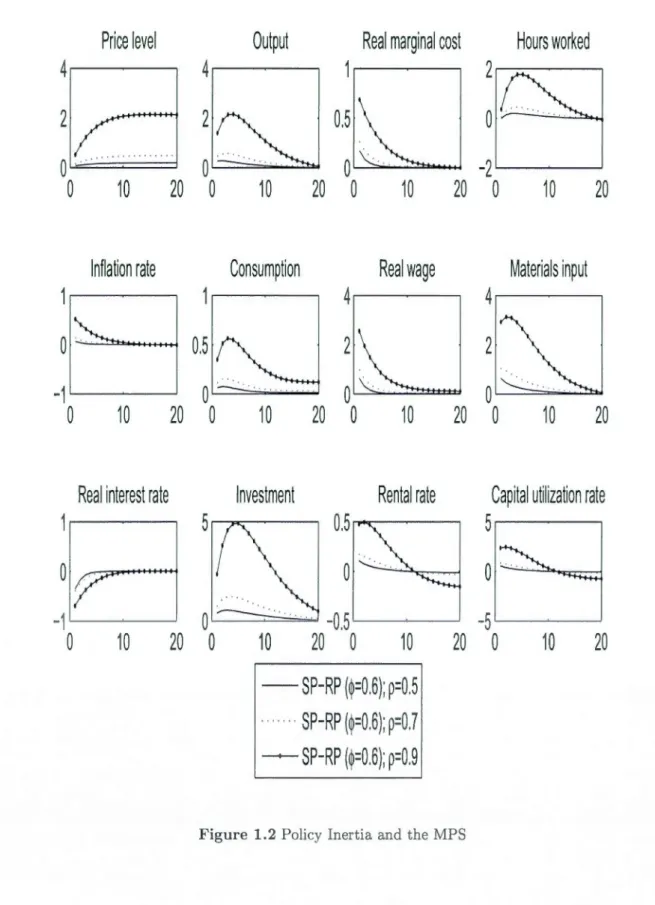
Endogenous monetary policy plays a key role in these findings, especially the degree of policy inertia. We find that the higher the interest-rate smoothing parameter in the policy rule is, the larger, more persistent and hump-shaped are the responses of aggregate

quantities to a monetary policy shock. Since this parameter is found to be high in recent

the MPS. 2

But despite severa! interesting implications, the sticky-price mode! with a roundabout production structure is plagued by two important anomalies. A first one is that employ-ment fluctuations ought to be associated with much smaller variations in the real wage (Lucas and Rapping, 1969). For instance, empirical evidence sa ys th at the real wage weakly rises following an expansionary monetary policy shock (Christiano, Eichenbaum and Evans, 1997, 2005). In contrast, the sticky-price mode! with materials input pre-diets the real wage strongly increases following an expansionary policy shock. A second anomaly is that while movements in materials input ought to be roughly proportionate to value-added and hours over the business cycle (Dotsey and King, 2006), the mode! predicts materials input fluctuates much more than value-added and hours.

To overcome these shortcomings, we activate a sticky-wage channel (see section 5). While leaving other main findings intact, adding sticky wages helps dampen the response of real wage and magnify movements in value added and hours relative to movements in materials input. With roundabout production, sticky wages and sticky priees, the mar-ginal cast of firms has three components. Two of these-the intermediate input priee and the wage index-are rigid. Thercfore, the marginal cast is Jess responsive to a monetary policy shock with sticky wages and sticky priees than with priee sitickiness alone. Thus, priees are more sluggish and the responses of aggregate quantities to a monetary policy shock stronger.

Other substantive findings can be summarized as follows. When assuming that the me-dian waiting ti me between priee adjustments is relatively short ( only 4.3 months) as microeconomie evidence by Bils and Klenow (2004) suggests, we find that a monetary policy shock still generates persistent and hump-shaped responses in aggregate quant i-ties. On the other hand, if the frequency of wage adjustment is set to be much lower

2. For instance, Smets and Wouters (2007) report an estimate for the interest-rate smoothing parameter of 0.81 for postwar U.S., and Justiniano and Primiceri (2008), an estimate of 0.85. Gali and Gertler (2007) argue that this parameter is weil above 0.6 empirically and can be as high as 0.9.

12

than the frequency of priee adjustment as microeconomie evidence by Barattieri, Basu

and Gottschalk (2010) suggests, we show that the real wage remains weakly procycl i-cal at the onset of a monetary policy shock. Furthermore, when accounting for neutra!

technology and investment-specific technology shocks (see section 6), we find that the investment-specific technology shock, like the monetary policy shock, generates per -sistent and hump-shaped responses of aggregate quantities, a weakly procyclical real

wage, and roughly proportionate movements in materials input, value-added and hours. In contrast, neutra! technology shocks give rise to a short-run decline in hours and an increase in output. We conclude that monetary policy and investment-specific techno -logy shocks stand as plausible sources of the strong positive comovement between hours and output observed during the postwar period, but not neutra! technology shocks.

1.2 The Model

The economy is populated by a large number of households, each endowed with a diff e-rentiated labor skill indexed by i E [0, 1] and by a large number of firms, each producing

a differentiated good indexed by j E [0, 1]. A government conducts monetary policy.

1.2.1 The Model

Denote by Lt a composite of differentiated labor skills Lt(i) for ·i E [0, 1] such that

Lt

=

[JJ

Lt(i)(a-1_{)/a di]af(a-}1_{), and by Xt a composite of differentiated goods Xt(j) for}

j E [0, 1] such that Xt

=

[JJ

Xt(J)(O-l)/O dj]IJ!(Ii-l), where 0' E (1, oo) and

e

E (1, oo) are the elasticity of substitution between the skills and between the goods, respertively. Both the composite skill and the composite good are produced in a perfectly competitive aggregate sector.

optimizing behavior in the aggregation sector are respectively given by

Lf(i) (1.1)

Xf(j)

=

where W1 is the wage rate of the composite skill which is related to the wage rates Wt(i)

for i E [0, 1] of the differentiated skills by W1 =

[JJ

W1(i)(l-a-)dijl1(1-a), and

Pt

is the

priee of the composite good related to the priees Pt (j) for j E [0, 1] of the differentiated goods by P₁

=

[JJ

Pt(.j)(l-e)qjjl/(1-e).

While the composite skill serves only as an input for the production of each differentiated good, the composite good serves either as a final consumption or investm nt good, or as an intermediate production input. The production of good j requires the use

of intermediate goods, effective capital services and labor as inputs. The production

function for a good of type

.i

is given by

otherwise,

(1.2) where f1(j) is the input of intermediate goods,

K1

(j) and L1(j) are the inputs of capital services and the composite skill, and F is a fixed cost which is identical across firms and ensures that profits are zero in the steady state. We rule out entry into and exit out of the production of good j. The parameter cjJ E (0, 1) measures the elasticity of output with respect to intermediate input, and the parameters ex E (0, 1) and (1 - ex) are the elasticities of value-added with respect to the capital services and labor inputs.

Each firm acts as a price-taker in the input markets and as a monopolistic competitor in the product market. A finn can choose the priee of its product, taking the demand

schedule in (1.1) as given. Priees are set according to the mechanism spelled out in Calvo (1983). In each period, a firm faces a constant probability 1- Çp of reoptimizing its priee,

with the ability to reoptimize being independent across firms and time. A firm that can reoptimize its priee will do so before the realization of the policy shock at time t.

14

A firm j set ting a new priee at date t chooses P1 (.j) to maximize its profits

00

Et

2)

çpr-t

Dt,T[Pt(j)X~(j) - V(X~(j))], (1.3) T=t

where E is an expectations operator, and Dt,T is the priee of a dollar at time T in units

of dollars at time t and V(X~(j)) is the cost ofproducing X~(j), equal to VT[X~(j)+F],

with VT denoting the marginal cost of production at time T.

Solving the profit-maximization problem yields the following optimal pricing decision

rule

( 1.4)

This rule says the optimal priee is a constant markup over a weighted average of the

marginal costs for the periods the priee will remain effective.

Solving the firm's cost minimization problem yields the following marginal cost function :

( 1.5)

where

{fi

is a constant term determined by cjJ and a, and R~ is the nominal renta! rate on

capital services. With roundabout production, the marginal cost function records three

components (PT, R~ and WT ). The impact on marginal cost of assuming input-output linkages among firms increases with the share of materials input c/J. Without roundabout

production ( cjJ

=

0), the marginal cost function records on! y two components ( R~ and

The conditional demand functions for the intermediate input and for the primary factor inputs used in the production of Xf+T (j) and derived from cost-minimization are

r

( .)

= A-

v

T

[X~(j)

+

F]

T J 'P PT ' (1.6)

R (:)

=

(1 - A-) VT[X~(j)

+

F]

and

(1.8)

A finn which is not allowed to reoptimize its priee in a given period nonetheless chooses the inputs of the intermediate good, capital services and the composite labor that

mini-mize production cost.

1.2.2 Monopolistically Competitive Households and Staggered Wage Dec

i-si ons

Each household i has a subjective discount factor (3 E (0, 1) and a utility function

E

L

(31 log(Ct(i) - bC1_l) - TJ t z ,

00 { Ld(

")l+X

}

t=O 1 +X

(1.9) where C1(i) is individual consumption, C1_ 1 is past-period aggregate consumption, b

>

0

measures the relative importance of habit formation, and Lf(i) is the demand schedule

for the household 's labor skills given by ( 1.1).

The budget constraint that household i faces at time t is

Pt[C1(i)

+

I1(i)

+

a(Zt(i))Kt(i)]

+

EtDt,t+lBt+I(i)

:S

Wt(i)Lf(i)

+

R~ Kt(i)

+

Ilt(i) + B,.(i)

+

Tt(i),

(1.10)

where Bt+l (i) is household i's holdings of a nominal bond representing a daim to one dollar in t

+

1 and costs Dt,t+l dollars at time t, W1(i) is the nominal wage rate for

labor skill of type i, Lf(i) is a demand schedule for type i labor specified in (1.1), R~ is

a nominal renta! rate on capital services, P1a(Z1(i))K1 (i) is the cost of changing capital utilization, 111(i) is household i's profit share, and T1('i) is a lump-sum transfer the household i receives from the government.

The physical capital accumulation equation is

Kt(i)

=

(

1

-

o)Kt_I(i)

+

[1

-

S

(~:

~~ili)

)]

ft(i), (1.11) where ois the physical rate of depreciation, ft(i) denotes time t purchases of investment

16

The amount of effective capital the households can rent to the firms is

(1.12) where Z1(i) denotes the utilization rate of capital. We impose two restrictions on the

capital utilization function a(Zt(i)) : the rate of capital utilization in the steady state equals one and a(1) =O.

Each household acts as a price-taker in the goods market and a monopolistic competitor in the labor market. It chooses consumption Ct(i), hours worked L1(i), bonds Bt(i),

investment ft(i) and capital utilization Z1(i) that maximize (1.9) subject to (1.10) and a borrowing constraint B1+I(i)

2:

- B, for sorne large positive number B. The initial

conditions on bond and capital are given.

It can also set a nominal wage for its differentiated tabor skill, taking the demand schedule (1.1) as given. The probability that a household sets a new wage is 1 - Çw. At date t

, for

a household i setting a new wage, its optimal choice of nominal wage is

(1.13)

where M RS denotes the marginal rate of substitution between leisure and incarne. Equa-tion (1.13) says the optimal wage is a constant markup over a weighted average of the

M R.S's for the periods the wage rate will remain effective. 3

1.2.3 Endogenous Monetary Policy

The monetary authority follows the Taylor rule :

(1.14) where 1ft= log( Pt/ Pt_I), 9Yt

=

log(Yi/Yi-d and ér,t is an i.i.d. normal process, with a zero mean and a fini te variance; a symbol- over a variable x denotes the deviation of x

from its steady-state value. The monetary policy rule (1.14) states that the monetary authority systematically reacts to deviations of inflation and output growth from targets

while smoothing short-term movements in the nominal interest rate (see also Erceg and

Levine, 2003; Gali and Rabanal, 2004; Liu and Phaneuf, 2007).

1.2.4 Equilibrium and Market-Clearing Conditions

An equilibrium for this economy consists of allocations C1(i),

K

1(i), Bt+1(i), Z1(i) and

wage W1(i) for household i, for ali i E [0,

1],

allocations ft(.j), Kt(.j), L1(.j) and priee P1(.i)

for firm j, for ali j E [0, 1], together with priees Dt,t+ 1, ?1, R~, and W₁, satisfying the

following conditions : (i) taking the wages and ali priees but its own as given, each firm's allocations and priee solve its maximization problem; (ii) taking priees and ali wages but

its own as given, each household's allocations and wage solve its utility maximization problem; (iii) markets for bonds, capital, the composite labor and the composite good clear; (iv) monetary policy is as specified.

We assume that (implicit) state-contingent financial contracts insure each household

against the idiosyncratic income risk that may arise from the staggering of wage ad

-justments. As in Rotemberg and Woodford (1997), Huang, Liu and Phaneuf (2004) and

Christiano, Eichenbaum and Evans (2005), such financial arrangements ensure that eq

ui-librium consumption and investment are identical across households, although nominal

wages and hours worked may differ. Under this assumption, we have

JJ

Yt(i)di

=

Y1 for

ali i. Given this relation, along with (1.6), the market-clearing condition

JJ

Yt(i)di

+

J6

ft(.j)d,j = Xt for the composite good implies that equilibrium real GDP is related to gross output by

(1.15) where G1

J

J

[P

t

(j) / Pt]-f! dj captures the priee-dispersion effect of staggered priee

con tracts.

The market-clearing conditions are

J6

Kf(j)dj

=

JJ

K1(i)di

=

K1 for capital services

18

(1.7) - (1.8) imply that equilibrium aggregate capital services and composite skill are related to gross output by

(1.16)

( 1.1 7)

Equations (1.15), (1.16) and (1.17), together with the price-setting equation (1.4) and the wage-setting equation (1.13), characterizes an equilibrium.

The overall resource constraint of the economy is

(1.18)

1.3 Parameter Calibration

The parameters we need to calibrate include the subjective discount factor (3, the pref e-rence parameters band

x,

the technology parameters cp and a, the elasticity of substi tu-tion between differentiated goods

e

and between differentiated la bor skills (J) the capital depreciation rateS, the investment adjustment cost parameter K-, the capital utilization elasticity Œa, the probability of priee non-reoptimization ~P> the probability of wage

non-reoptimization Çw, and the monetary policy parameters Pr, Prr, py and C!o:,.· 4 The values assigned to these parameters are summarized in Table 1.1.

Following the standard business cycle literature, we set (3

=

0.99,

x

=

2, and

o

=

0.025 implying an annualized real interest rate of 4 percent in the steady state, an intertemporal elasticity of labor hours of 0.5, and an annual capital depreciation rate of 10 percent. We set the coefficient of habit formation b to 0.8 (Fuhrer, 2000; Boldrin,

Christiano and Fisher, 2001). The investment adjustment cost parameter r;, is fixed at 3 (Christiano, Eichenbaum and Evans, 2005), and the capital utilization elasticity C!a at

4. The parameter rJ in the utility function ha.s no effect on equilibrium dynamics (in the log-linearized equilibrium system) and thus we do not need to a.ssign a particular value to it.

1.5 (Basu and Kim bail, 1997; Dotsey and King, 2006). With zero steady-state profits,

the parameter a: corresponds to the share of payments to capital in total value-added in the National Incarne and Product Account (NIPA), implying a= 0.4 (see also Cooley and Prescott, 1995).

The elasticity of substitution between differentiated goods B determines the steady-state

markup of priees over marginal cost, with a markup of()/ ( ()- 1). Rotemberg and Wood

-ford (1997) assume a value-added markup of 1.2, implying B = 6. Christiano, Eichen

-baum and Evans (2005) estimate the value-added markup at 1.2 in a mode! controlling

for variable capital utilization. Nakamura and Steinsson (2010) assume B = 4 and a value-added markup of 1.33 in a menu-cost mode! featuring roundabout production. We set B = 6, so the value-added markup is 1.2. Similarly, we set the elasticity of subst

i-tution between differentiated labor skills CJ = 6 (Huang and Liu, 2002; Huang, Liu and Phaneuf, 2004).

The paramctcr cf; measures the share of payments to intermediate input in total produc -tion cost or cost share. With markup pricing, it equals the product of the steady-state

markup and the share of intermediate input in gross output or revenue share. We rely

on two different sources of data to calibrate cf; for the postwar U.S. economy. The first source is a study by Jorgenson, Gollop and Fraumeni (1987) suggesting that the revenue share of intermediate input in total manufacturing output is about 50 percent. With a

steady-state markup of 1.2, this implies cf; = 0.6. The second source relies on the 1997

Benchmark Input-Output Tables of the Bureau of Economie Analysis (BEA, 1997). In

the Input-Output Table, the ratio of "total intermediate" to 11_{total industry output}11 in the manufacturing sector or revenue share is 0.68. With a steady-state markup of 1.2, this implies cf;

=

0.816. Admissible values of cf; bence range between 0.6 and 0.816. Huang, Liu and Phaneuf (2004) and Nakamura and Steinsson (2010) choose cf;

=

0.7. Here, we take a conservative stand and set the baseline value of cf; at 0.6. Later, we assess the sensitivity of our findings to higher values of cf;. 5

20

The parameter Çp measures the probability of priee non reoptimization. In a survey of U.S. priee behavior, Taylor (1999) documents that priees have changed about once a year on average during the postwar period. Recent evidence based on U.S. microeconomie data suggests otherwise. Using summary statistics from the Consumer Priee Index micro data compiled by the U.S. Bureau of Labor Statistics for 350 categories of consumer goods and services, Bils and Klenow (2004) document that the median waiting time between priee adjustments is 4.3 months when taking into account priee changes during temporary sales, while it is 5.5 months when they are excluded from the sample. Cogley and Sbordone (2008, footnote 19) argue that when approximating the waiting time to the next priee change by Ç~, the median waiting time between priee adjustments is given by - ln(2)/ ln(Çp)· Setting Çp

=

2/3 would therefore imply that the median waiting time between priee changes is 5.1 months.

We consider our choice of é,p

=

2/3 as conservative, and this for the following reasons. The most detailed evidence reported in Bils and Klenow (2004) covers only the years 1995-1997. Using Jess disaggregated priee data, they report evidence showing that é,p was higher for the years 1959-2000 (see Bils and Klenow, 2004, Table 4 and Figures 2 and 3). Also, Nakamura and Steinsson (2008) show that when priee changes occuring during temporary sales and those associated with product substitutions are excluded from the sample, then priees remain effective for 8- 11 months, while including priee changes for product substitutions, priees remain effective for 7- 9 months. Therefore, Çp could have been higher than 2/3.

As for the probability of wage non reoptimization, é,w, it is chosen as follows. A study by Barattieri, Basu and Gottschalk (2010), that exploits a panel of micro data from the Survey of Income and Program Participation for the years 1996-1999, suggests nominal wages have changed less frequently than priees. Based on their estimates, they argue the average duration of wage contracts relevant for the calibration of macroeconomie models should be around 16.6 months. On the other hand, macroeconomie studies report estima tes of (,w implying an average duration of wage contracts between 3 and 4 quarters

we consider evidence from micro or macro studies, nominal wages seem to adjust Jess

frequently than priees. Therefore, when our madel will account bath for sticky wages

and sticky priees, we set Çw = 3/4. Later, we examine the consequences on our findings

of widening the gap between é,p and Çw as micro evidence seems to suggest.

Finally, the parameters of the Taylor rule are set as follows : Pr = 0.8, p.,. = 1.5 and

py

=

0.125. These values are broadly consistent with recent estimates reported in Smets

and Wouters (2007) and Justiniano and Primeceri (2008), and with the calibration in

Christiano, Eichenbaum and Evans (2005). The standard deviation of the monetary

policy shock ur is set at 0.004 (Ireland, 2007).

1.4 Staggered Price-Setting and the MPS

Basu (1995) argues that the interplay between intermediate goods used in an input

-output structure and sticky priees can give rise to a multiplier for priee stickiness (MPS).

He works from a demand-driven state-dependent mode! with menu costs of changing

priees and no capital accummulation. In this section, we assess Basu's contention using

a version of the mode! described above that combines input-output linkages between

firms, staggered priee contracts, flexible wage decisions and endogenous monetary policy.

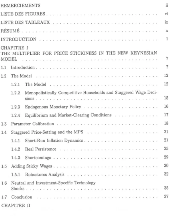
We are interested in the effects of the MPS on inflation inertia and the persistence of

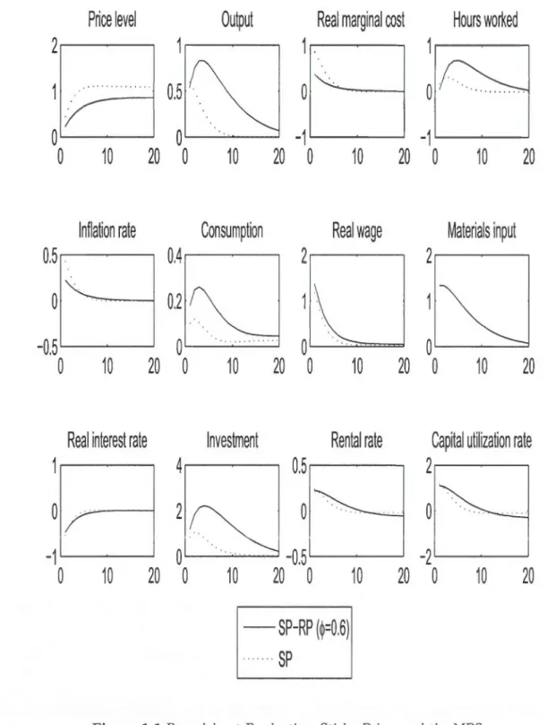
aggregate quantities in response to monetary policy shocks. Figure 1.1 displays the

impulse-response functions of the following variables to a 1-percent negative shock to

the nominal interest rate :

- the priee leve!, the inflation rate and the real interest rate;

- output, consumption and investment ;

- the real marginal cost, the real wage rate and the renta! rate;

- hours worked, materials input and capital utilization.

1.4.1 Short-Run Inflation Dynamics

Severa! impulse responses are significantly different when the input-output production structure interacts with priee stickiness and endogenous monetary policy. Without

ma-22

terials input, the marginal cost function (1.5) records two components, the rentai rate on capital services and the wage index. These two components are flexible, so inflation reacts strongly to the policy shock and is weakly persistent. With input-output linkages between firms, the marginal cost function records a third component in the form of the rigid intermediate input priee, which has for effect of reducing the sensitivity of margi -nal cost to the policy shock. The increase in marginal cost is more than 2 times smaller with materials input on impact of a positive monetary policy shock. Priees rise more gradually towards their new higher steady-state leve!, and inflation is more persistent.

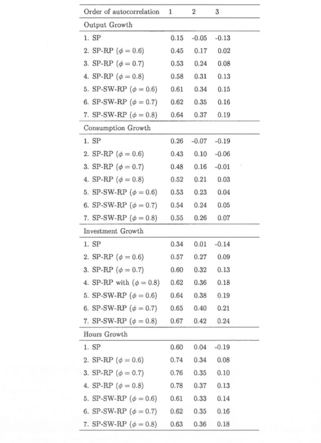
Another way to assess the quantitative importance of the MPS is by generating the autocorrelation functions of inflation implied by the sticky-price models with and w i-thout intermediate goods in the spirit of the test proposed by Fuhrer and Moore (1995) and Nelson (1998). Fuhrer and Moore report evidence showing th at rational expecta -tions models featuring overlapping wage contracts (Phelps, 1978; Taylor, 1980) generate weakly persistent inflation. To provide a better fit of the data, they propose a fr ame-work in which agents care about relative real wages (Buiter and Jewitt 1981). This setup implies that higher-order backward-looking elements enter the wage contract, resulting in a much higher seriai correlation of inflation. However, the contracts in Fuhrer and Moore are not cast within explicit individual optimization problems for households and firms.

Nelson (1998) performs a similar exercise, but for a wider range of models featuring sticky priees, including new keynesian pricing models with microfoundations. Nelson examines whether this class of models is able to replicate the high and slowly decaying positive autocorrelations of the quarterly first difference of the log U .S. GDP deflator. Among the models Nelson examines, only those of Fuhrer and Moore (1995) and King and Watson (1996) imply a high seriai correlation of inflation. Fuhrer and Moore rely on ad hoc backward-looking elements, whereas King and Watson (1996) assume that priees adjust once every 2.5 years on average, which is implausible in light of evidence on priee behavior from microeconomie studies.

Table 1.2 reports the autocorrelations of the quarterly first difference of the log nonfarm business sector implicit priee deflator (NBD) and of the log GDP implicit priee deflator

(GDPD) for the years 1959 :1-2007 :III. 6 _{We also report in this table the autocorrelations}

of the quarterly first difference of the log compensation of the nonfarm business sector (NBC) and of the log average hourly earnings of priva te industries (AHEP). 7 _{The firs}

t-order autocorrelations of priee inflation are above 0.8, and they remain positive and high beyond the first lag. The autocorrelations of wage inflation are also high, but they are somewhat higher with the nominal wage measured by the AHEP.

Tables 1.3 and 1.4 compare the autocorrelations of priee inflation and wage inflation

implied by the sticky-price models including and excluding roundabout production. The

autocorrelations of priee inflation are denoted by Prr(k) for k = 1, ... , 6, with Prr(k) representing the k1horder of autocorrelation of priee inflation. Those corresponding to wage inflation are denoted by Pw(k) for k = 1, ... , 6. For the sake of cornparison, we also include the autocorrelations of priee inflation of the Fuhrer and Moore ( 1995) and King and Watson (1996) models as they were generated by Nelson (1998).

Without input-output linkages, the mode! predicts a first-order autocorrelation of priee

inflation of 0.65, and rapidly decaying autocorrelations beyond the first !ag. When

inter-mediate goods are included in the mode!, these autocorrelations are significantly higher. Specifically, Prr(1) = 0.814 and the higher-order autocorrelations decay Jess rapidly. Now, recall that these findings are obtained for a share of intermediate goods of 0.6, while the admissible values range from 0.6 to 0.816. We also report the autocorrelations correspon-ding to q;

=

O. 7 and 0.8. Increasing the value of

q;

enhances the autocorrelations of priee inflation. The first-order theoretical autocorrelations are respectively 0.83 for

q;

= 0.7,

and 0.85 for

q;

=

0.8. Note that the autocorrelations for k

=

5, 6 are now importantly higher than in Fuhrer and Moore's mode!, but that they are somewhat smaller than in

6. Our sample period ends before the so-called Great Recession of 2007 :4-2009 :4.

7. The non-farm business compensation has been used in Christiano, Eichenbaum and Evans (2005), and the average hourly earnings of private industries in Gertler and Trigari (2009).

24

King and Watson's model. Since wage decisions are flexible, the seria! correlation of wage

inflation is weak. Nonetheless, the seria! correlation of priee inflation is high, confirming

that the MPS arising from the interactions between intermediate goods and sticky priees

is an important mechanism generating inflation inertia.

Other approaches have been followed in the literature to account for short-run inflation

dynamics. To better track actual inflation, Gali and Gertler (1999) suggest incorporating

lagged inflation into the NKPC equation. In their mode!, firms are allowed to reset their

priees upon reeeiving a Calvo signal. Firms receiving this signal are divided in two groups.

One group sets new priees optimally in a purely forward-looking fashion, whereas the

other group follows a simple rule of thumb. Rule-of-thumbers set new priees equal to

average priees in the most recent round of priee adjustment, plus a correction for previous

period inflation. They are therefore backward-looking. The backward-looking term helps

tracing short-run inflation dynamics.

Christiano, Eichenbaum and Evans (2005) use a slightly different setup, assuming instead

full backward indexation of wages and priees in a DSGE mode! featuring Calvo wage and

priee contracts. Firms reoptimize their priees upon reeeiving the appropriate stochastic

signal. When allowed to reoptimize, they set priees optimally in a purely forward-looking

manner. The remaining firms not authorized to reoptimize their priees will nonetheless

index them to last period inflation. Households are similarly divided in two groups. A

first group of households set wages optimally upon receiving a stochastic signal allowing

them to do so, while the other group not entitled to wage reoptimization index them to

last period inflation. Smets and Wouters (2007) use a similar indexing mechanism. The use of backward-looking elements in DSGE models has been criticized by Woodford

(2007), Sbordone (2007), Cogley and Sbordone (2008) and Chari, Kehoe and McGr

at-tan (2009). One criticism is that these assumptions cannot be linked to the optimizing

behavior of households and firms. Another criticism specifie to backward indexation is

that when used in conjunction with Calvo contracts, this assumption implies that all

light of micro level evidence reported by Bils and Klenow (2004) and Nakamura and

Steinsson (2008), among others. Assuming that all wages in the economy change every 3 months is just as implausible (Barattieri, Basu and Gottschalk, 2010).

Cogley and Sbordone (2008) follow a different approach. Based on a number of studies

that mode! U.S. trend inflation as a driftless random walk (Cogley and Sargent, 2005;

Stock and Watson, 2007), they incorporate variations in trend inflation into an otherwise

NKPC mode!. In general equilibrium, trend inflation ought to be determined by the

long-run target in the central bank's po licy rule (Ire! and, 2007). Wh en accounting for time-varying trend inflation, estimates of backward indexation turn out to be statistically insignificant. Furthermore, the frequency of priee adjustment is broadly consistent with microeconomie evidence.

1.4.2 Real Persistence

We next turn our attention to the adjustment of aggregate quantities in response to

a monetary policy shock implied by both sticky-price models. In a thought provoking

paper, Chari, Kehoe and McGrattan (2000) (CKM) argue that once incorporated into

business cycle mode! built from solid microfoundations, staggered priee contracts fail

to generate persistent output fluctuations in response to a monetary policy shock. This

anomaly, known as the persistence problem, bas launched a rapidly growing literature

aimed at identifying new sources of output persistence in DSGE models. To generate their findings, CKM first estimate the impulse response of output to the shock in a

univariate autoregression mode!. They measure output persistence by the time after a

policy shock for the deviation of output from trend to shrink to half of its impact value.

Then, they approximate the impact of staggered priee contracts on output persistence

by the contract multiplier, computed as the ratio of the half-life of output deviations

after a monetary shock with staggered price-setting to the corresponding half-life with

flexible priee decisions. So defined, the contract multiplier conveys information mostly