Mechanical structures and thermal management scheme for HiCIBaS's stratospheric balloon mission

(1)

Mechanical structures and thermal management

scheme for HiCIBaS's stratospheric balloon mission

Mémoire

Deven Patel

Maîtrise en physique - avec mémoire

Maître ès sciences (M. Sc.)

(2)

Résumé

Le projet HiCIBaS (High-Contrast Imaging Balloon System) est une mission de télescope à ballon dirigé dans le but de l'imagerie exoplanète en utilisant des techniques à contraste élevé. Pour la première mission en 2018, les principaux objectifs étaient de développer les systèmes nécessaires et de valider leurs performances, d'acquérir des données de vol et de prouver la capacité de survie de tous les systèmes et composants majeurs dans des conditions proches de l'espace.

Ce projet de maîtrise porte sur deux aspects de la charge utile: la conception de la monture de télescope alt-az dynamique pour le système de pointage et le développement des sangles thermiques personnalisées pour le système optique. La monture du télescope est la structure qui supporte le télescope et permet aux moteurs du système de pointage de le diriger vers la position souhaitée. Les sangles thermiques personnalisées sont une solution développée pour dissiper la chaleur générée par les principaux composants du système optique (caméras, contrôleurs, etc.). Les deux solutions ont été testées lors d’un vol de nuit en août 2018 dans le cadre de la campagne STRATOS de l’agence spatiale canadienne à Timmins, en Ontario. Ce mémoire définira les exigences des deux systèmes, présentera le développement des conceptions, détaillera les analyses et les tests effectués, démontrera la conformité aux exigences, commentera sur les performances de la mission et donner des conseils des moyens d'améliorer les deux conceptions pour les futures itérations du projet.

(3)

Abstract

The HiCIBaS (High-Contrast Imaging Balloon System) project is a balloon-borne telescope mission with the big-picture goal of exoplanet-imaging using high-contrast techniques. For the scope of the pilot mission in 2018, the main goals were to develop the necessary systems and validate their performance, acquire flight data, and prove the survivability of all systems and major components in near-space conditions.

This Master’s project deals with two aspects of the overall payload: the design of the dynamic alt-az telescope mount for the pointing system and the development of the custom thermal straps for the optics system. The telescope mount is the structure that supports the telescope and allows the pointing system’s motors to direct it to the desired position. The custom thermal straps are a solution that was developed to dissipate the heat generated by the optics system’s main components (cameras, controllers, etc.). Both solutions were tested during an overnight flight in August of 2018 under the Canadian Space Agency’s STRATOS campaign in Timmins, Ontario. This mémoire will define the requirements for both systems, present the development of the designs, detail the analyses and tests performed, demonstrate conformance to the requirements, comment on mission performances, and provide insight on ways to improve both designs for future iterations.

(4)

List of Figures

Figure 1: Example of high-contrast techniques used for exoplanet-imaging (Kaufman, 2017) ... 1

Figure 2: The effect of atmospheric turbulence on incoming starlight wavefronts (Buscher, 2015) ... 2

Figure 3: Final design of the HiCIBaS mount structure ... 7

Figure 4: Intersection of the three main axes on the Nasmyth mirror ... 8

Figure 5: Positioning of the Nasmyth mirror in relation to the telescope’s flange ... 9

Figure 6: Clearance between mount structure (at ±20◦ azimuth positions) and gondola structure ... 10

Figure 7: Clearance between mount structure (at 60° altitude position) and gondola structure ... 10

Figure 8: Mount structure descent position (-20° altitude, 0° azimuth) ... 11

Figure 9: Length and height of mount structure at 0° altitude and azimuth position ... 12

Figure 10: Width of mount structure at 0° altitude and azimuth position ... 12

Figure 11: Position of mount structure’s interface plate on gondola’s front floor... 13

Figure 12: Horizontal clearance of mount structure from the edge of CARMEN’s front floor ... 13

Figure 13: Center of gravity position of the standalone mount structure ... 15

Figure 14: Center of gravity position of the mount structure in the CARMEN gondola ... 15

Figure 15: Operational load limits of the RM-3 motor ... 16

Figure 16: RM-3 assembly configuration (left) and resulting free-body diagram (right) ... 17

Figure 17: Operational load limits of the RM-8 motor ... 18

Figure 18: RM-8 assembly configuration (left) and resulting free-body diagram (right) ... 18

Figure 19: RM-5 coupling assembly configuration (left) and resulting free-body diagram (right) ... 19

Figure 20: Maximum Von-Mises stress due to impact simulation of telescope arm structure ... 23

Figure 21: Maximum Von-Mises stress from the impact simulation of the standing structure ... 25

Figure 22: Interface plate with assigned numbering scheme for the insert screws ... 27

Figure 23: Maximum Von-Mises stress from the 1G static simulation of the structure ... 29

Figure 24: Maximum displacement from the 1G static simulation of the structure ... 29

Figure 25: Stress convergence curve for the full-assembly structural simulation ... 31

Figure 26: Distribution of aspect ratios of the standing structures simulation model ... 32

Figure 27: Distribution of element quality for the standing structures simulation model ... 33

Figure 28: Landing environment of the gondola... 35

Figure 29: Fabrication and assembly procedure of the custom thermal strap solution ... 41

Figure 30: Custom thermal strap post-fabrication and assembly ... 42

Figure 31: Full CAD model displaying the optical bench’s cover ... 43

Figure 32: Polyurethane foam integrated on the interior of the cover ... 44

Figure 33: Full assembly configuration of the optics bench ... 45

Figure 34: Critical surface for the HNü 512 Detector ... 45

Figure 35: Full assembly configuration of the HNü 512 Detector ... 45

Figure 36: Critical surface for the Space Controller ... 46

Figure 37: Full assembly configuration of the Space Controller ... 46

Figure 38: Critical surface for the HNü 512 Regulator ... 47

Figure 39: Full assembly configuration of the HNü 512 Regulator ... 47

Figure 40: Critical surface for the HNü 128 Detector ... 48

Figure 41: Full assembly configuration of the HNü 128 Detector ... 48

Figure 42: Critical surface for the HNü 128 Controller ... 49

Figure 43: Full assembly configuration of the HNü 128 Controller ... 49

Figure 44: Thermal resistance network and derived equations for the HNü 128 Controller ... 51

(6)

Figure 46: Comparison of the simulation results and the lab test results ... 54

Figure 47: Modified meshing scheme for the HNü 512 Regulator components ... 55

Figure 48: Convection coefficient curve used for the flight simulation ... 56

Figure 49: Ambient temperature curve used for the flight simulation ... 57

Figure 50: Altitude profile of the mission used for the flight simulation ... 58

Figure 51: Simulation model of the thermal system’s main components (and cover hidden) ... 59

Figure 52: Heat convergence curve for the full-assembly thermal simulation ... 61

Figure 53: Distribution of aspect ratios for elements of the thermal simulation model ... 62

Figure 54: Distribution of element quality for elements of the thermal simulation model ... 62

Figure 55: Final assembly of the thermal system integrated into the gondola (cover removed) ... 63

Figure 56: Thermocouple placement for the 512 Detector strap ... 65

Figure 57: Simulation vs. mission comparison of 512 Detector strap’s performance ... 65

Figure 58: Thermocouple placement for the 128 Detector strap ... 66

Figure 59: Simulation vs. mission comparison of 128 Detector strap’s performance ... 66

Figure 60: Thermocouple placement for the 128 Controller strap ... 67

Figure 61: Simulation vs. mission comparison of 128 Controller strap’s performance ... 67

Figure 62: Thermocouple placement for the 512 Regulator strap ... 68

Figure 63: Simulation vs. mission comparison of 512 Regulator strap’s performance ... 68

Figure 64: Thermocouple placement for the Space Controller strap ... 69

Figure 65: Simulation vs. mission comparison of Space Controller’s performance ... 69

Figure 66: Thermocouple placement for the Bench ... 70

Figure 67: Simulation vs. mission comparison of Bench’s performance ... 70

Figure 68: Adjusted convection coefficient curve for post-flight simulations ... 72

Figure 69: Adjusted ambient temperature curve for post-flight simulations ... 72

Figure 70: Approximate altitude profile of the flight for the entire duration of the mission ... 73

Figure A1: Manufacturer’s datasheet for the RM-3 motor (Newmark Systems, 2018) ... 80

Figure A4: Insert load specifications (Centre National d’Études Spatiale, 2018) ... 83

Figure A5: Design criteria defined in CSA Safety Regulations Document (Mathieu, 2013) ... 84

Figure A6: Impact loads measured during mission (Centre National d’Études Spatiale, 2018) ... 85

Figure A7: Supplier’s datasheet for the copper shim stock (McMaster-Carr, 2018) ... 86

Figure A8: Manufacturer’s datasheet for the thermal epoxy (OMEGA, 2018) ... 87

Figure A9: Supplier’s datasheet for polyurethane foam (McMaster-Carr, 2018) ... 88

Figure A10: Supplier datasheet for polyurethane foam (Federal Foam Technologies, 2007) ... 89

Figure A11: Supplier’s datasheet for thermal interface material (McMaster-Carr, 2018) ... 90

Figure A12: Manufacturer’s datasheet for thermal interface material (Henkel-Adhesives, 2015) ... 91

(7)

List of Tables

Table 1: Mount structure requirements ... 5

Table 2: Weight distribution of the mount structure components ... 14

Table 3: Maximum stresses experienced by the screws supporting the telescope... 24

Table 4: Force reactions for the screws interfacing the mount structure to the gondola’s floor .... 26

Table 5: Results of calculation for the force equation criterion ... 28

Table 6: Summary of numerical results for the standing mount structure ... 34

Table 7: Summary of simulation results for the standing mount structure... 34

Table 8: Maximum acceleration loads experienced at separation and landing ... 36

Table 9: Thermal system requirements ... 39

Table 10: Maximum ∆T values allowed for each strap component ... 52

Table 11: Actual ∆T values to be expected for each strap component ... 52

Table 12: Breakdown of heat flow inputs for the flight simulation ... 56

Table 13: Maximum temperatures expected through simulation for critical surfaces ... 60

(8)

List of Abbreviations and Acronyms

CAD Computer-aided design

CCD Charge-coupled device

CNES Centre National d’Études Spatiale

CSA Canadian Space Agency

DM Deformable mirror

EMCCD Electron-multiplying charge-coupled device HiCIBaS High-Contrast Imaging Balloon System LOWFS Low-order wavefront sensor

OAP Off-axis parabolic

SOW Scope of work

(9)

Introduction

Scientific Context

In the realm of astronomy, high-contrast imaging is a technique used to detect faint objects, such as exoplanets, that are in proximity to bright sources, such as stars. Typically, this is accomplished using a coronagraph, an instrument that physically blocks a star from the view of a detector, suppressing its starlight (Kaufman, 2017). With less light present in the field of view, the detector will be less saturated, and the faint objects can more effectively be detected. This is demonstrated in Figure 1 with the HR 8799 star suppressed in the center and the 4 exoplanets exposed (denoted as b, c, d, and e).

Figure 1: Example of high-contrast techniques used for exoplanet-imaging (Kaufman, 2017)

Even with this technique, ground-based telescopes encounter difficulties with exoplanet imaging due to “astronomical seeing,” a phenomenon caused by atmospheric turbulence (MacRobert, 2006). Earth’s atmosphere is composed of several different layers that each have drastically different air properties and environmental conditions. This results in differing optical refractive indices throughout the atmosphere and that effects the way light is refracted, causing the image taken on-ground to be blurry. Since atmospheric turbulence is dynamic, the light’s wavefront is constantly being aberrated, as demonstrated by Figure 2, causing it to appear as if it is “twinkling” because of the variation of light intensity from one moment to the next; this phenomenon is also known as scintillation. Atmospheric turbulence in the troposphere (closest to the ground) is the hardest to predict and, therefore, plays the biggest role in atmospheric seeing.

b

d

c

(10)

Figure 2: The effect of atmospheric turbulence on incoming starlight wavefronts (Buscher, 2015)

Astronomical seeing can be overcome, though, using advanced optical instrumentation and by using techniques to countermeasure the aberrations caused, as seen with the advent of adaptive optics in astronomy. However, another strategy can be used to circumvent the problem altogether: performing the imaging outside of Earth’s atmosphere.

Purpose of HiCIBaS

The big-picture goal of Université Laval’s High-Contrast Imaging Balloon (HiCIBaS) project is to perform exoplanet imaging from the stratosphere, effectively eliminating the worst contributor to astronomical seeing (the troposphere) by being above 99.996% of the air in Earth’s atmosphere. A successful mission would have multiple benefits, not limited to just the performance of high-contrast imaging and airborne telescopes. Space-based telescopes are extremely costly and, for those that don’t venture into deep space, a cheap alternative can be high-altitude observations. Sub-orbital flights are also much more practical as they can be recovered, maintained or modified, and relaunched. With the introduction of newer technologies for space-based telescopes, high-altitude balloon flights offer a unique platform for near-space conditions for testing and system design validation purposes, even if the flight duration will be significantly shorter than an orbital mission.

However, to realize this long-term goal, there are many functional issues linked to high-altitude observations, that need to be addressed. One of the biggest issues is pointing stability. For ground-based telescopes, the use of a coronagraph is highly effective because the telescope itself is relatively stable and typically only moving in very small increments in altitude and azimuth directions. A high-altitude balloon, though, is constantly moving in 3D space in the stratosphere, as well as moving in altitude and azimuth directions to track a star. This causes the performance of the optical system to be dependent on the performance of the pointing system. Pointing errors can result in contrast degradation in two ways: jitter and stability error, and imperfect centering of the coronagraph on the target star. Jitter and stability error would cause wavefront errors generated by beam-walk and imperfect centering of the coronagraph would cause starlight leaking onto the detector; both contributing to contrast degradation (Université Laval, 2016).

(11)

Another major challenge is designing systems while lacking reliable data surrounding the high-altitude environment. Air properties and ambient temperatures vary significantly based on geographical location, altitude and day-to-day meteorology. As a result, atmospheric turbulence, and the aberrations caused by it, are impossible to define and to design for. A prior mission, a pilot mission, is required to characterize these conditions and their effects on: temporal variability, scintillation, coherence cell diameter, transmission, and stray or scatted light (Université Laval, 2016).

In the case of both challenges, a Low-Order Wavefront Sensor (LOWFS) is something that can be used. Very simply, a LOWFS is an optical system that measures wavefront errors caused by low-order optical aberrations (defocus, etc.) and aids in their correction by sending data to another optical component, or system, that can correct for them. For HiCIBaS, the LOWFS can serve as fine-pointing correction to mitigate stability problems and keep the coronagraph centered on the target star.

Objectives of the HiCIBaS Mission

In order to achieve the short-term goals, necessary for the long-term vision, outlined in section 1.2, HiCIBaS has 5 specific objectives for the pilot mission (Université Laval, 2016):

1. Develop and test a promising new type of Low-Order Wavefront Sensor (LOWFS).

2. Develop and test a generic precision pointing telescope system that can be used in future missions requiring sub-milli-arcsecond level pointing (e.g. high-contrast imaging missions).

3. Measure and gather data on the wavefront instabilities and errors encountered at 40 km of altitude in the visible region of the spectrum (scientific interest).

4. Test optical components (DM, coronagraph) for future high-contrast imaging missions. 5. Fly in space-like conditions the LOWFS including a Nuvu EMCCD camera.

Objectives of the Project

This project involves the mechanical aspects of the payload. More specifically, the mandate for the mechanical specialist of this project was to:

1. Design a dynamic alt-az mount that is capable of supporting a 14” telescope.

2. Design a thermal system capable of dissipating the heat generated by the detectors, controllers and voltage regulator (of the Nüvü Cameras’ components).

The first mandate pertains directly to the 2nd_{objective of the HiCIBaS mission because it involves the} development of the mechanical structure that is required for the pointing system. The second mandate supports the 4th_{and 5}th_{objectives of the mission by ensuring the proper operation and performance of the associated} systems.

Both solutions will be discussed in-depth in Chapters 1 and 2, respectively, of this memoir. In them, the low-level requirements will be defined, the final designs and motivating factors will be reviewed, the analyses

(12)

and simulations performed will be detailed and discussed, the mission performance will be evaluated, and, finally, ways to improve both designs will be advised.

Chapter 1: Dynamic Telescope Mount Structure

1.1 Scope of Work (SOW)

The dynamic telescope mount structure is one of the two main structures of the HiCIBaS project (the optics bench being the second). The mount structure serves two main purposes: to accommodate the front-end optics (telescope, Nasmyth mirror, etc.) and to provide a dynamic platform for the pointing system to guide the telescope. In other words, this structure is directly contributing towards the success of Objective 2.

More specifically, the telescope mount structure must:

1. Demonstrate structural integrity, as defined by the Canadian Space Agency (CSA) and Centre National d’Études Spatiale (CNES).

2. Respect the maximum weight limit, as defined by CNES.

3. Provide the necessary degrees of freedom in altitude and azimuth direction, as required by the pointing system.

4. Respect the dimensional and positional restrictions of the front-end optics, as required by the optics system.

5. Accommodate the components of, both, the pointing system and the optics system, as required by the respective specialists.

This chapter will detail the work done for the telescope mount structure and aim to demonstrate conformance to the scope of work defined above. Specifically, the requirements will be defined, followed by a discussion and description of the final design, an evaluation of the design with the approaches taken and the validation criteria, the mission performance of the structure, and, finally, recommendations for further improvement.

(13)

1.2 System Requirements

Table 1: Mount structure requirements

Requirement # Requirement Origin

1 The telescope and Nasmyth mirror central axes must intersect on _{the center of the tertiary mirror to a precision of 0.5 mm} Optics System 2 The Nasmyth mirror and OAP mirror central axes must intersect _{on the center of the tertiary mirror to a precision of 0.5 mm} Optics System 3 The rotational axis of the RM5 motor must be coaxial to the _{Nasmyth mirror’s cylindrical mount to a precision of 0.5 mm} Optics System 4 The threaded flange (to mount optics) at the back of the telescope must be 121.141 mm from the tertiary mirror (center-to-center

distance) Optics System

5 The structure must never intersect with the optical axis at any _{point of the optics system} Optics System 6 The telescope must have ±20° of freedom in the azimuth direction _{with at least 20 mm of clearance at the extremities} Pointing System 7 The telescope must have +60° of freedom in the altitude direction _{with at least 20 mm of clearance at the extremity} Pointing System

8 The telescope must have at least -20° of freedom in the altitude direction and zero clearance from the descent support at the

extremity Pointing System

9 The maximum weight placed on the gondola’s floor must be less _{than or equal to 100 kg} CNES 10 The operational load limits of the RM-3, RM-5, and RM-8 motors (as defined on their respective datasheets) must be met with a

safety factor of 1.2 or more Pointing System

11 The maximum normal load expected (P) on every insert of the _{gondola’s floor must be less than or equal to 1960 N (Pcrit)}₂ CNES 12 The maximum transverse load expected (Q) on every insert of the _{gondola’s floor must be less than or equal to 4080 N (Qcrit)}₂ CNES 13 The following equation must be satisfied for every insert of the _{gondola’s floor: (P/Pcrit)}₂_{+ (Q/Qcrit)}₂_{≤ 1}₂ CNES 14 The design yield load (DYL) must be less than or equal to the _{material’s tensile yield strength (YL): DYL ≤ YL}₃ CSA 15 The design ultimate load (DUL) must be less than or equal to the _{material’s tensile yield strength (YL): DUL ≤ YL}₃ CSA 16 The load limit (LL) multiplied by 1.5 must be less than or equal to _{the material’s tensile yield strength (YL): LL × 1.5 ≤ YL}₃ CSA 1 _{As defined in the material datasheets for each of the respective motors (Appendix 1)}

2_{As defined in the CARMEN_Insert_loads document (Appendix 2) provided by CNES and CSA.} 3_{As defined in the CSA-STRATOS-RPT-0004-A-EN document (Appendix 3) provided by CSA.}

(14)

Just as important as defining the requirements themselves is their origin. Therefore, here is a brief breakdown of the motivation behind the requirements:

• Requirements 1-5: To provide the necessary positioning and tolerancing for the optical design concept and to ensure optimal performance of the optical system.

• Requirements 6-8: To provide the necessary degrees of freedom for the pointing system to track and follow the movement of the targeted star over the duration of the mission.

• Requirement 9: To demonstrate adherence to the maximum allowable weight supported by the CARMEN gondola’s floor.

• Requirement 10: To demonstrate the capability of the motors to perform their respective tasks for their respective applications.

• Requirement 11-13: To demonstrate adherence to the load limits of the M6 inserts on the CARMEN gondola’s floors imposed by CNES.

• Requirement 14-16: To demonstrate structural integrity of the mount structure to the CSA for safety reasons.

1.3 System Design

1.3.1 Design Breakdown and Driving Factors

This section will highlight the key factors considered during the design phase of the mount structure and how they played in role in design and component choices made during its development.

In terms of the overall, large-scale design, the mount structure was made to respect the dimensional constraints of the CARMEN gondola while also respecting the degrees of freedom required to track the desired stars for the science aspect of the HiCIBaS project (the latter is discussed in Section 2.3.3). However, five major factors influenced the physical dimensions and geometry of the design:

1. Implementing the “three-axes” design concept that was imposed by the optical system and pointing system (discussed in Section 2.3.2).

2. Positioning of the optical components (discussed in Section 2.3.2).

3. Respecting the weight limit imposed by CNES (discussed in Section 2.3.4).

4. Achieving the rigidity required to withstand the increased loads experienced at balloon separation and landing (discussed in Section 2.4).

5. Accommodating the pointing system’s motors and the front-end optical components. Figure 3 provides a look at the final design of the mount structure and its major components.

(15)

Figure 3: Final design of the HiCIBaS mount structure

To comment on some of the components of the design, the components of the mount structure in Figure 1 have been color-coded:

• Red: Shield (made of 6061-T6 aluminum alloy) for jettisoned stainless-steel balls during descent. • Black: 14” Schmidt-Cassegrain telescope (Celestron: C14-AF-XLT) used to collect the light required to

perform science and tracking tasks.

• Green: Mirror mount (ThorLabs: POLARIS-K3S5) housing the 2” Nasmyth mirror; aptly named for its purpose of guiding the incoming light (from the telescope) straight downwards and towards the rest of the optical system.

• Yellow: Rotary stage motors (Newmark: RM-3, RM-5, RM-8) used to deliver the arcsecond precision desired in azimuth and altitude.

• Blue: CCD camera (IDS: UI-3060CP Rev.2) and scope for the pointing system used to provide a wider view of the sky, and to locate and track the desired star(s).

• Light Grey: Alt-Az mount structure (made of 6061-T6 aluminum alloy) using a bracketed design that is made to be rigid and lightweight.

• Orange: Constant-force springs (McMaster: 9293K14) used to balance the telescope on the altitude axis to relieve stress on the altitude axis’ rotary stage motor (RM-5).

• Purple: Support posts (made of 6061-T6 aluminum) to reduce impact loads on RM-8 motor during separation and landing events.

Not shown in Figure 3 are the deep groove ball bearings that are used to support the top portion of the structure and the telescope and allow free rotation on the altitude axis; the grease in these bearings are replaced with vacuum-compatible grease to survive the environmental conditions of the stratosphere.

(16)

1.3.2 Optical Design Considerations

This section aims to show a more in-depth look at the considerations made for the optical system in the design phase; in the process, it will also show conformance to Requirements 1-5 that were defined to ensure those considerations are met.

The mount structure is simply a means for the pointing system to accomplish its task of tracking the target star so that the optical system can perform the science of the mission. In that regard, the optical system has the most influence (top-level) on the mechanical design of the mount structure, as mentioned in section 2.3.1, making it a driving factor.

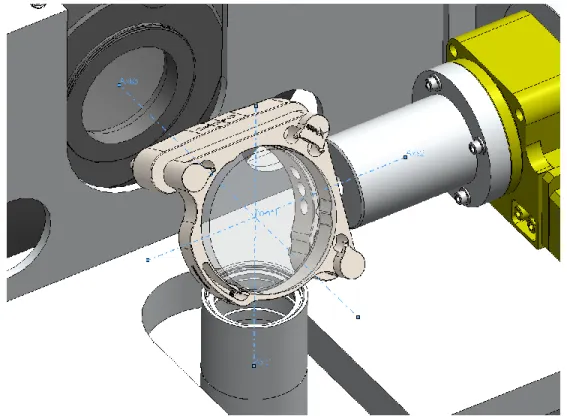
The first major consideration for the optical system is the “three-axes” concept. This concept involves intersecting the optical axis of the telescope and the rotational axes of the altitude and azimuth motors onto a single mirror (the aforementioned “Nasmyth” mirror), as shown in Figure 4. Attached to this design concept is the precision to which the axes must intersect, as defined in Requirements 1-3.

This concept serves one major purpose: to render the mount and “front-end” optical design fixed for future missions, allowing the “back-end” optical system to be modifiable or even replaced by entirely different optical systems (turnkey operation). In other words, different optical missions could be developed in parallel and flown during the same or subsequent flight campaigns. This would also facilitate the design process since half of the mechanical design would be complete, lessening the time needed to develop a payload.

(17)

The optics team was able to confirm during the testing phase that the three axes intersected as desired, which gives validation for the conformance to Requirements 1-3.

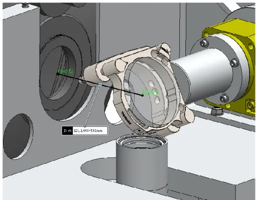
The second major consideration for the optical system is the positioning of various optical and mechanical elements. Most notably, for the placement of the Nasmyth mirror, as defined by Requirement 4 and as seen in Figure 5, and the movement of the mount’s back side during operation. Although these seem relatively minor, these two constraints (coupled with the three-axes concept) made the design of the structure difficult. On one hand, the placement of the Nasmyth mirror causes the center of gravity to be further from the center of rotation of the structure and elongating the overall length of the structure. On the other hand, to ensure that the structure does not intersect the optical path, the opposite side of the structure is restricted in length. The result is an asymmetric structure that would require more counterweights to be added to counteract the weight of the telescope that is further away. This was eventually mitigated using the constant-force springs solution mentioned in Section 2.3.1, it is discussed at length in Section 2.4.4.

Figure 5: Positioning of the Nasmyth mirror in relation to the telescope’s flange

1.3.3 Pointing System Considerations

This section will show the range capabilities of the telescope mount structure and the clearance from the gondola structure at all extremities.

The pointing system directly impacts optical performance and, therefore, the science of the mission. The mount structure must be designed, therefore, to accommodate the pointing system’s needs so that the optical system can perform the science without restrictions from internal systems. In order to track the targeted stars, the pointing system requires specific degrees of freedom: ±20° in the azimuth direction and -20° to +60° in the

(18)

altitude direction. For safety concerns, a clearance of 20 mm at all extremities of these ranges must be met, as well.

Figures 6, 7, and 8 show the required range capabilities of the mount structure and the clearance from the gondola structure for ±20° azimuth, 60° altitude, and -20° altitude, respectively.

Figure 6: Clearance between mount structure (at ±20◦ azimuth positions) and gondola structure

(19)

Figure 8: Mount structure descent position (-20° altitude, 0° azimuth)

The actual degrees of freedom of the mount structure and clearances from the gondola structure were confirmed to be accurate to those shown in Figure 6-8 during integration and testing to a magnitude of ±2 mm. This discrepancy was expected and comes from the positional tolerance of the gondola’s floor and the positional adjustment of the gondola’s floor needed for optical alignment. In all cases, however, the clearance was confirmed to be greater than or equal to 20 mm, the minimum desired clearance. Requirements 6-8 were, therefore, satisfied during the design phase and validated during integration and testing.

1.3.4 Overall Geometry and Positioning

This section will show the overall geometry and dimensions of the telescope mount structure and its placement in the CARMEN gondola.

Figures 9 and 10 demonstrate the overall dimensions of the entire mount structure at 0° altitude and azimuth. Figure 11 shows the positioning of the interface plate and the M6 inserts that are engaged on the CARMEN gondola’s floor; this is important information for CNES to assess the mount structure’s impact on the weight balance for the gondola. Figure 12 shows how far the telescope clears the edge of the gondola; there was no constraints imposed for this, but it is information that was requested by the CSA for safety reasons.

(20)

Figure 9: Length and height of mount structure at 0° altitude and azimuth position

(21)

Figure 11: Position of mount structure’s interface plate on gondola’s front floor

(22)

1.3.5 Weight and Center of Gravity (CG) Position

This section will provide a breakdown of the weight supported by the front floor of the CARMEN gondola; it will serve to demonstrate conformance to Requirement 9. The front floor will be occupied by the mount structure assembly and the telescope descent support; the breakdown provided in this section will show the weight contribution of the various main parts of the mount structure.

The weight distribution and CAD model versus actual structure weight difference is demonstrated by Table 2. Note that there is a ~6 kg difference between the actual weight (measured) and the CAD weight (expected). Since the entire telescope structure was measured while fully assembled, the origin of this discrepancy is unclear. However, it is most likely a result of the lower material density of the actual mount structure (i.e. the bulk of the mass) than was inputted, and estimated, in the CAD model.

Figures 9 and 10 provide information regarding the position of the CG of the mount structure with respect to its own physical center and with respect to the gondola’s floor, respectively. As with the positioning of the mount structure, this is relevant information for CNES regarding weight balance of the gondola.

Table 2: Weight distribution of the mount structure components

Parts CAD Weight (kg) Actual Weight (kg)

Telescope 26.040

87.364

Telescope Brace Structure 10.233

Standing Structure 22.478

Rotary Motors (RM8, RM5, RM3) 18.600

Rotating Baseplate 6.986

Interface Plate 7.553

Auxiliary Components (fasteners,

supports, etc.) 1.182

(23)

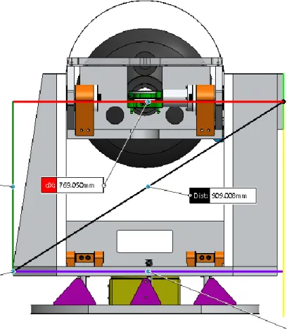
Figure 13: Center of gravity position of the standalone mount structure

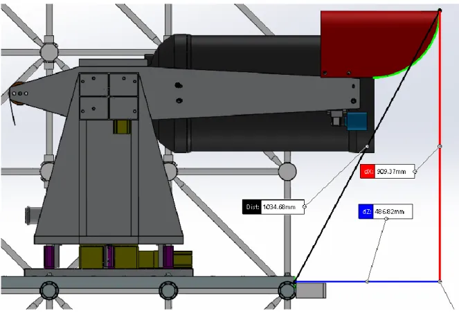
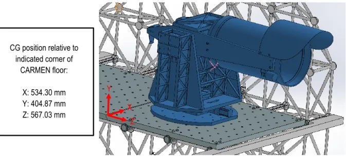
Figure 14: Center of gravity position of the mount structure in the CARMEN gondola

It is clear by looking at Table 2 that Requirement 9 was met during the design phase and validated to be conform in the testing phase, regardless of the discrepancy. Also, although it was not a requirement, Figures 9 and 10 demonstrate that the CG of the mount structure is very close to the center of the gondola’s floor (only 34.3 mm away) between the walls of the gondola. This means that it’s well-positioned in the gondola and the

CG position relative to the intersection point of mount’s azimuth axis and the top surface

of the CARMEN: X: -22.68 mm Y: 404.87 mm Z: 172.03 mm Y X Z CG position relative to indicated corner of CARMEN floor: X: 534.30 mm Y: 404.87 mm Z: 567.03 mm Y X Z

(24)

structure itself has good symmetry, which is an important design feature when dealing with dynamic structures and increased load scenarios.

1.4 Evaluation of the Design

This section will demonstrate conformance to Requirements 10-16 pertaining to the general structural requirements of the mount structure and the load limit of the CARMEN M6 inserts, and increased loads experienced at landing. All designs in this section were made in SolidWorks 2017 and imported into ANSYS 18.0 for structural simulation. All calculations were done in accordance to section 5.4.2 of CSA’s Safety Regulations for Aerostat Design and Operations document (CSA-STRATOS-RPT-0004-A-EN).

1.4.1 Numerical Analyses

The numerical analyses performed in this section all utilize the same strategy: removing parts of the structure surrounding the area of interest, making a free-body diagram, performing the necessary calculations to determine the resultant forces, torques, and moments, and, finally, evaluating the design.

1.4.1.1 RM-3 Motor – Moment Load Analysis

As mentioned in section 2.3.1, the RM-3 motor is responsible for controlling the orientation of the Nasmyth mirror in the altitude direction. The motor is mounted with its rotational axis being coaxial with the rotational axis of the mount structure’s entire top portion (i.e. the rotational axis of the RM-5 motor). This section will demonstrate how the operational load limits of the RM-3 motor was respected. The complete datasheet for the motor is shown in Appendix 1, but, for convenience, the operational load limits are shown in Figure 15.

Figure 15: Operational load limits of the RM-3 motor

The main concern for the RM-3 motor is the moment load since it is holding 3 components in a cantilever configuration, as shown in Figure 16. Since the CG of these components is centered very close to the rotational axis and are of relatively low mass, the normal and torque loads are negligible in terms of criticality.

(25)

Figure 16: RM-3 assembly configuration (left) and resulting free-body diagram (right) 𝑇𝑜𝑡𝑎𝑙 𝑤𝑒𝑖𝑔ℎ𝑡 𝑜𝑓 𝑠𝑢𝑝𝑝𝑜𝑟𝑡𝑒𝑑 𝑐𝑜𝑚𝑝𝑜𝑛𝑒𝑛𝑡𝑠 (𝐹𝑐𝑜𝑚𝑝𝑜𝑛𝑒𝑛𝑡𝑠): 0.71 𝑘𝑔 = 6.9651 𝑁 𝐷𝑖𝑠𝑡𝑎𝑛𝑐𝑒 𝑜𝑓 𝑡𝑜𝑡𝑎𝑙 𝑤𝑒𝑖𝑔ℎ𝑡 𝐶𝐺 𝑡𝑜 𝑅𝑀 − 3 (𝐷𝐶𝐺_𝑐𝑜𝑚𝑝𝑜𝑛𝑒𝑛𝑡𝑠) = 60.128 𝑚𝑚 = 0.060128 𝑚 𝑀𝑜𝑚𝑒𝑛𝑡 (𝑀𝑟𝑒𝑠𝑢𝑙𝑡𝑎𝑛𝑡) = 𝐹𝑜𝑟𝑐𝑒 (𝐹𝑐𝑜𝑚𝑝𝑜𝑛𝑒𝑛𝑡𝑠) × 𝐷𝑖𝑠𝑡𝑎𝑛𝑐𝑒 (𝐷𝐶𝐺_𝑐𝑜𝑚𝑝𝑜𝑛𝑒𝑛𝑡𝑠) = 0.4188 𝑁𝑚 𝑴𝒐𝒎𝒆𝒏𝒕 𝑳𝒐𝒂𝒅: 𝐹𝑎𝑐𝑡𝑜𝑟 𝑜𝑓 𝑆𝑎𝑓𝑒𝑡𝑦 (𝐹𝑜𝑆) = 13.5 𝑁𝑚 0.4188 𝑁𝑚= 32.23 ≥ 1.2 (𝑚𝑖𝑛𝑖𝑚𝑢𝑚 𝐹𝑜𝑆 𝑑𝑒𝑠𝑖𝑟𝑒𝑑) With an FoS of 32.23, we have more than enough confidence to state that the operational load limits of the motor are respected.

1.4.1.2 RM-8 Motor – Normal and Moment Load Analysis

As mentioned in section 2.3.1, the RM-8 motor is responsible for controlling the orientation of the entire mount structure in the azimuth direction. This section will demonstrate how the operational load limits of the RM-8 motor was respected. The complete datasheet for the motor is shown in Appendix 1, but, for convenience, the operational load limits are shown in Figure 17.

(26)

Figure 17: Operational load limits of the RM-8 motor

The main concerns for the RM-8 motor are the normal and moment loads since it is holding most of the components that make up the mount structure, as shown in Figure 18. Since there are no forces or moments causing a torque, the torque loads can be neglected in terms of criticality.

Figure 18: RM-8 assembly configuration (left) and resulting free-body diagram (right)

𝑇𝑜𝑡𝑎𝑙 𝑤𝑒𝑖𝑔ℎ𝑡 𝑜𝑓 𝑠𝑢𝑝𝑝𝑜𝑟𝑡𝑒𝑑 𝑐𝑜𝑚𝑝𝑜𝑛𝑒𝑛𝑡𝑠 (𝐹𝑐𝑜𝑚𝑝𝑜𝑛𝑒𝑛𝑡𝑠): 71.213 𝑘𝑔 = 698.6 𝑁 𝑵𝒐𝒓𝒎𝒂𝒍 𝑳𝒐𝒂𝒅: 𝐹𝑎𝑐𝑡𝑜𝑟 𝑜𝑓 𝑆𝑎𝑓𝑒𝑡𝑦 (𝐹𝑜𝑆) = 317 𝑘𝑔 71.213 𝑘𝑔= 4.451 ≥ 1.2 (𝑚𝑖𝑛𝑖𝑚𝑢𝑚 𝐹𝑜𝑆 𝑑𝑒𝑠𝑖𝑟𝑒𝑑) 𝐷𝑖𝑠𝑡𝑎𝑛𝑐𝑒 𝑜𝑓 𝑡𝑜𝑡𝑎𝑙 𝑤𝑒𝑖𝑔ℎ𝑡 𝐶𝐺 𝑡𝑜 𝑅𝑀3 (𝐷𝐶𝐺_𝑐𝑜𝑚𝑝𝑜𝑛𝑒𝑛𝑡𝑠) = 150.712 𝑚𝑚 = 0.150712 𝑚 𝑀𝑜𝑚𝑒𝑛𝑡 (𝑀𝑟𝑒𝑠𝑢𝑙𝑡𝑎𝑛𝑡) = 𝐹𝑜𝑟𝑐𝑒 (𝐹𝑐𝑜𝑚𝑝𝑜𝑛𝑒𝑛𝑡𝑠) × 𝐷𝑖𝑠𝑡𝑎𝑛𝑐𝑒 (𝐷𝐶𝐺_𝑐𝑜𝑚𝑝𝑜𝑛𝑒𝑛𝑡𝑠) = 105.29 𝑁𝑚 𝑴𝒐𝒎𝒆𝒏𝒕 𝑳𝒐𝒂𝒅: 𝐹𝑎𝑐𝑡𝑜𝑟 𝑜𝑓 𝑆𝑎𝑓𝑒𝑡𝑦 (𝐹𝑜𝑆) = 135.5 𝑁𝑚 105.29 𝑁𝑚= 1.287 ≥ 1.2 (𝑚𝑖𝑛𝑖𝑚𝑢𝑚 𝐹𝑜𝑆 𝑑𝑒𝑠𝑖𝑟𝑒𝑑)

M

F

(27)

With FoS’s of 4.451 and 1.287 for the normal and moment loads, respectively, we have enough confidence to state that the operational load limits of the motor are respected for normal operation. For impact during landing, the increased load felt (up to 15 g) would drop our FoS below 1.2 for both limits. In order to avoid this, support posts were integrated in the design to transfer the impact to the interface plate and gondola floor below and, consequently, relieve the RM-8 motor of this increased load.

1.4.1.3 Altitude-Direction Coupling – Torque Load Analysis

As mentioned in section 2.3.1, the altitude-direction coupling is responsible for transferring the torque from the RM-5 motor to the top portion of the mount structure (i.e. the structure that supports the telescope), as seen in Figure 19. In other words, the RM-5 motor controls the movement of the top portion of the mount structure in the altitude direction. Since the top portion of the mount structure is supported by bearings on both sides, the normal loads experienced by the RM-5 motor itself are negligible in terms of criticality; however, the coupling still encounters a significant torque load that must be considered. Therefore, this section will show the analysis that determined the maximum torque that would be experienced by the coupling, to compare it to how much it is designed to handle. The complete datasheet for the coupling and RM-5 motor are shown in Appendix 1, but, for convenience, the allowable torque limit for the coupling is 10 Nm and the maximum torque output for the RM-5 motor is 12.RM-5 Nm; therefore, the coupling is the bottleneck of the design.

Figure 19: RM-5 coupling assembly configuration (left) and resulting free-body diagram (right)

We start with a balance of forces of the top portion of the structure to determine the resultant torque to apply to the coupling:

𝐿𝑜𝑎𝑑 𝑎𝑝𝑝𝑙𝑖𝑒𝑑 𝑑𝑢𝑒 𝑡𝑜 𝑠𝑝𝑟𝑖𝑛𝑔 𝑡𝑒𝑛𝑠𝑖𝑜𝑛 (𝐹𝑠𝑝𝑟𝑖𝑛𝑔) = 18.55 𝑘𝑔 = 182 𝑁 𝐶𝐺 𝑑𝑖𝑠𝑡𝑎𝑛𝑐𝑒 𝑓𝑟𝑜𝑚 𝑟𝑜𝑡𝑎𝑡𝑖𝑜𝑛𝑎𝑙 𝑎𝑥𝑖𝑠 (𝐷𝐶𝐺_𝑠𝑝𝑟𝑖𝑛𝑔) = 0.298 𝑚 𝑅𝑒𝑠𝑢𝑙𝑡𝑎𝑛𝑡 𝑡𝑜𝑟𝑞𝑢𝑒 (𝑇𝑠𝑝𝑟𝑖𝑛𝑔) = 𝐹𝑜𝑟𝑐𝑒 (𝐹𝑠𝑝𝑟𝑖𝑛𝑔) × 𝐷𝑖𝑠𝑡𝑎𝑛𝑐𝑒 (𝐷𝐶𝐺_𝑠𝑝𝑟𝑖𝑛𝑔) = 54.236 𝑁𝑚 𝐿𝑜𝑎𝑑 𝑎𝑝𝑝𝑙𝑖𝑒𝑑 𝑑𝑢𝑒 𝑡𝑜 𝑤𝑒𝑖𝑔ℎ𝑡 𝑜𝑓 𝑡𝑒𝑙𝑒𝑠𝑐𝑜𝑝𝑒 (𝐹𝑡𝑒𝑙𝑒𝑠𝑐𝑜𝑝𝑒) = 26.04 𝑘𝑔 = 255.45 𝑁 𝐶𝐺 𝑑𝑖𝑠𝑡𝑎𝑛𝑐𝑒 𝑓𝑟𝑜𝑚 𝑟𝑜𝑡𝑎𝑡𝑖𝑜𝑛𝑎𝑙 𝑎𝑥𝑖𝑠 (𝐷𝐶𝐺_𝑡𝑒𝑙𝑒𝑠𝑐𝑜𝑝𝑒) = 0.244 𝑚

T

(28)

𝑅𝑒𝑠𝑢𝑙𝑡𝑎𝑛𝑡 𝑡𝑜𝑟𝑞𝑢𝑒 (𝑇𝑡𝑒𝑙𝑒𝑠𝑐𝑜𝑝𝑒) = 𝐹𝑜𝑟𝑐𝑒 (𝐹𝑡𝑒𝑙𝑒𝑠𝑐𝑜𝑝𝑒) × 𝐷𝑖𝑠𝑡𝑎𝑛𝑐𝑒 (𝐷𝐶𝐺_𝑡𝑒𝑙𝑒𝑠𝑐𝑜𝑝𝑒) = 62.33 𝑁𝑚

𝑅𝑒𝑠𝑢𝑙𝑡𝑎𝑛𝑡 𝑡𝑜𝑟𝑞𝑢𝑒 𝑜𝑛 𝑡ℎ𝑒 𝑐𝑜𝑢𝑝𝑙𝑖𝑛𝑔 (𝑇𝑟𝑒𝑠𝑢𝑙𝑡𝑎𝑛𝑡) = 62.33 − 54.236 = 8.094 𝑁𝑚 𝑻𝒐𝒓𝒒𝒖𝒆 𝑳𝒐𝒂𝒅: 𝐹𝑎𝑐𝑡𝑜𝑟 𝑜𝑓 𝑆𝑎𝑓𝑒𝑡𝑦 (𝐹𝑜𝑆) = 10 𝑁𝑚

8.094 𝑁𝑚= 1.235 ≥ 1.2 (𝑚𝑖𝑛𝑖𝑚𝑢𝑚 𝐹𝑜𝑆 𝑑𝑒𝑠𝑖𝑟𝑒𝑑) With an FoS of 1.235, we have enough confidence to state that the operational load limit of the coupling is respected.

1.4.2 Simulation Analyses

This section will highlight the simulations performed for various critical parts of the mount structure, followed by brief discussions on the results.

The simulations performed in this section utilize a similar strategy as seen for the numerical analyses in Section 2.4.1: simplifying the structure surrounding the area of interest in the CAD model (discussed in Section 2.4.2.1), applying the appropriate parameters, constraints, and loads (discussed in Section 2.4.2.1), running the simulation, and, finally, analyzing the accuracy of the results (discussed in Section 2.4.2.6).

1.4.2.1 General Simulation Setup and Analysis

1.4.2.1.1 Simulation Setup

The primary goal of this section is to build confidence in the setup of the simulations performed. More specifically, to build confidence in the simulation model’s preparation and the parameters used. This section will outline the setup of the simulation by describing the general setup strategy, the input parameters, the parameter values, and the results expected.

To begin, the type of simulation chosen was the explicit dynamics simulation. This decision is the most appropriate since the loads experienced by the structure are impact loads. The general strategy for the simulations was to simplify the model as much as possible by removing parts to save simulation time, while retaining all the parts that may have a significant impact on the results. For some simulations, removing the parts also improved the accuracy of the simulation model. For example, the telescope arms and standing structure (Sections 2.4.2.1.4 and 2.4.2.1.5) were separated because the interaction between the two proved difficult to model correctly. To compensate, they were separated and constrained accordingly in each of their simulation conditions. All the parts that were removed were replaced with a single point mass located at the CG of all those parts combined and applied to the areas that they were connected to.

The next step was to ensure that the meshing of the components was well-generated. Meshing is the practice of breaking up a component into small pieces, called elements, to be solved by a finite element analysis through the software’s numerical solver. The meshing of components will directly impact the accuracy of the results. The overall goal is to generate a mesh that is fine enough to deliver accurate results, but coarse enough to minimize simulation time. For the general components that were typically larger, the mesh sizes were left to

(29)

the default sizes (up to 20 mm) determined by the software. If a load-bearing component or area was close to the critical path, or expected critical path, of the stress, mesh sizes were refined down to 0.1 to 5 mm. Mesh sizes were also refined for areas that presented higher level of structural error or lower levels of mesh quality, as discussed in Section 2.4.2.2. This was also the case for geometries that were more complex. Again, mesh sizes can be seen in Figures 20-24 for each simulation performed.

With the simulation model established, the loads of the simulation can be applied. In order to satisfy Requirements 11-16, the landing scenario is the determining factor for the loads applied since it is the worst-case scenario. Therefore, an acceleration load was applied to the simulation model, with 15 g in the vertical direction and 6.8 g in the lateral direction.

With the loads applied, the constraints must also be applied; this varied from simulation to simulation. For example, for the standing structure, the bottom of the base plate was fixed at the location of the bolts that held it in place and the area that it was resting on. For the interface plate, the bolts were fixed in place themselves. For the telescope mounting bolts simulation, the telescope arm was fixed. The constraints were made to simulate the physical model as accurately as possible.

Finally, the results desired must be defined. Again, this varies simulation to simulation. For most of them, the Von-Mises stress is the most important data because it can be used to show conformance to Requirements 14-16 and is, widely considered to be the most accurate means of determining the structural integrity of a ductile-material structure, since it is used to predict yield behavior. For the interface plate, where the force on the bolts was of prime concern, the force reactions was the desired data. In both cases, structural error is another result that was desired in order to perform one of the V&V activities outlined in Section 2.4.2.2.

1.4.2.2 Analysis Setup

In order to prepare the following sections for the results of the simulations performed, some context must be provided about the CSA’s Safety Data Pack (CSA-STRATOS-RPT-0004-A-EN), which can be found, in partial format, in Appendix 3, and how it outlines the approach to be taken to satisfy Requirements 14-16.

Section 5.3.2 of the CSA’s Safety Data Pack outlines the steps taken to prove structural integrity of a part using the maximum stress simulated (LL). This stress will be the Von-Mises stress since it better predicts the behavior of ductile metals. Safety factors defined by the CSA are then applied to this value to determine three design loads; the same three design loads required to satisfy Requirements 14-16 that can be found for each simulation. The following are the list of safety factors and the equations required to determine the design loads.

Safety factors as defined by the CSA: • Model factor (KM) = 1.4 • Project factor (KP) = 1.15 • Design factor (FOSD) = 1.2 • Yield factor (FOSY) = 1.25 • Ultimate factor (FOSU) = 1.5

(30)

Design load equations:

• DLL (Design Limit Load) = LL × KP × KM • DYL (Design Yield Load) = DLL × FOSY • DUL (Design Ultimate Load) = DLL × FOSU

(31)

1.4.2.2.1 Telescope Arm Structure and Screws (Top Section) – Stress Analysis

The telescope arm structure is the top section of the mount structure. It holds the telescope on one end and uses constant-force springs on the other end to balance the structure on the elevation axis. This structure was deemed important to analyze since it is holding the telescope (which is about a quarter of the total weight of the structure) and presents a big risk in the event of failure. There are two areas of interest for this simulation: the maximum stress on the structure itself and the stresses experienced by the eight screws supporting the telescope.

Using the strategy and parameters mentioned in Section 2.4.2.1, the simulation was performed, and the results are shown in Figure 20 and Table 3.

Figure 20 shows the maximum stress experienced by the structure of the telescope arms and the analysis that follows is done using the CSA’s criteria mentioned in Section 2.4.2.2.

Figure 20: Maximum Von-Mises stress due to impact simulation of telescope arm structure

𝐷𝑒𝑠𝑖𝑔𝑛 𝐿𝑖𝑚𝑖𝑡 𝐿𝑜𝑎𝑑 (𝐷𝐿𝐿) = 𝐿𝐿 × KM × KP × FOSD = 55.2 × 1.4 × 1.15 × 1.2 = 106.65 MPa 𝑫𝒆𝒔𝒊𝒈𝒏 𝒀𝒊𝒆𝒍𝒅 𝑳𝒐𝒂𝒅 (𝑫𝒀𝑳) = 𝐷𝐿𝐿 × FOSY = 106.65 × 1.25 = 𝟏𝟑𝟑. 𝟑𝟏 𝐌𝐏𝐚 ≤ 𝟐𝟕𝟔 𝐌𝐏𝐚 (𝐘𝐋) 𝑫𝒆𝒔𝒊𝒈𝒏 𝑼𝒍𝒕. 𝑳𝒐𝒂𝒅 (𝑫𝑼𝑳) = 𝐷𝐿𝐿 × FOSU = 106.65 × 1.5 = 𝟏𝟓𝟗. 𝟗𝟖 𝐌𝐏𝐚 ≤ 𝟑𝟏𝟎 𝐌𝐏𝐚 (𝐔𝐋) 𝑮𝒆𝒏𝒆𝒓𝒂𝒍 𝑺𝒂𝒇𝒆𝒕𝒚 𝑭𝒂𝒄𝒕𝒐𝒓 𝑪𝒉𝒆𝒄𝒌: 𝐿𝐿 × 1.5 = × 1.5 = 𝟖𝟐. 𝟖 𝐌𝐏𝐚 ≤ 𝟐𝟕𝟔 𝐌𝐏𝐚 (𝐘𝐋)

In order to satisfy Requirements 14-16, we can compare these results to the material’s tensile yield strength (YL). We see that the values are less than the material’s tensile yield strength (276 MPa) on all counts (DYL, DUL, and the general safety factor check) so the design is sufficiently strong; the results are summarized in table format in Section 2.4.3.2.

(32)

Table 3 summarizes the maximum stress experienced by each of the screws supporting the telescope with a comparison to their shear strength. The location of the screws is indicated by red dots in Figure 20.

Table 3: Maximum stresses experienced by the screws supporting the telescope

Location Maximum Shear Stress _{Experienced (MPa)} Shear Strength of _{Screws (MPa)} Factor of Safety

Front 7.215 1172.11 162.45 7.218 162.39 6.940 168.89 7.622 153.78 Back 11.228 104.39 11.712 100.08 10.72 109.34 11.515 101.79

With the maximum shear stress experienced by the screws significantly lower than their shear strength, it can be concluded that the 8 screws are sufficiently strong and distribute the load effectively enough to be safe. It is worth noting that the screws closer to the elevation axis are experiencing loads that are about 58% larger than those in the front. This is expected knowing that the center of gravity is closer to those screws but still interesting for future designs.

(33)

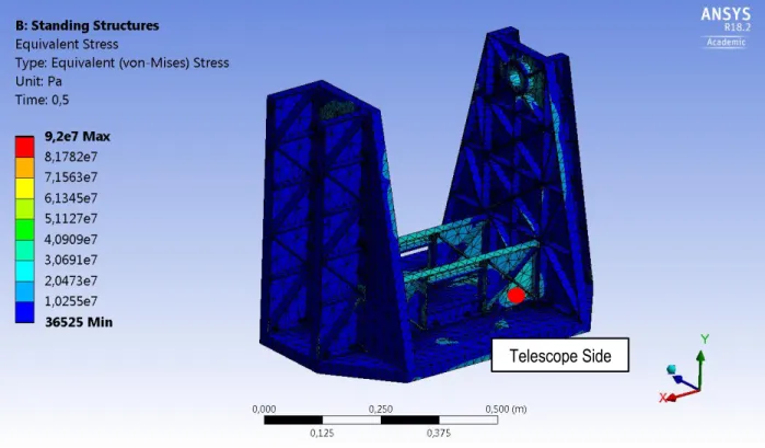
Standing Structure and Base (Mid Section) – Stress Analysis

The standing structure is the mid-level portion of the mount structure. This part of the design is an essential to the overall structural integrity of the mount. It was deemed important to analyze since it is supporting the entire top-portion of the structure (which is close to half of the weight of the entire mount), making it critical from a safety standpoint.

Using the strategy and parameters mentioned in Section 2.4.2.1, the simulation was performed, and the result is shown in Figure 21. The analysis that follows the simulation is done using the criteria mentioned in Section 2.4.2.2.

Figure 21: Maximum Von-Mises stress from the impact simulation of the standing structure

𝐷𝑒𝑠𝑖𝑔𝑛 𝐿𝑖𝑚𝑖𝑡 𝐿𝑜𝑎𝑑 (𝐷𝐿𝐿) = 𝐿𝐿 × KM × KP × FOSD = 92.7 × 1.4 × 1.15 × 1.2 = 179.10 MPa 𝑫𝒆𝒔𝒊𝒈𝒏 𝒀𝒊𝒆𝒍𝒅 𝑳𝒐𝒂𝒅 (𝑫𝒀𝑳) = 𝐷𝐿𝐿 × FOSY = 179.10 × 1.25 = 𝟐𝟐𝟑. 𝟖𝟖 𝐌𝐏𝐚 ≤ 𝟐𝟕𝟔 𝐌𝐏𝐚 (𝐘𝐋) 𝑫𝒆𝒔𝒊𝒈𝒏 𝑼𝒍𝒕. 𝑳𝒐𝒂𝒅 (𝑫𝑼𝑳) = 𝐷𝐿𝐿 × FOSU = 179.10 × 1.5 = 𝟐𝟔𝟖. 𝟔𝟓 𝐌𝐏𝐚 ≤ 𝟑𝟏𝟎 𝐌𝐏𝐚 (𝐔𝐋) 𝑮𝒆𝒏𝒆𝒓𝒂𝒍 𝑺𝒂𝒇𝒆𝒕𝒚 𝑭𝒂𝒄𝒕𝒐𝒓 𝑪𝒉𝒆𝒄𝒌: 𝐿𝐿 × 1.5 = 92.7 × 1.5 = 𝟏𝟑𝟗. 𝟎𝟓 𝐌𝐏𝐚 ≤ 𝟐𝟕𝟔 𝐌𝐏𝐚 (𝐘𝐋)

In order to satisfy Requirements 14-16, we can compare these results to the material’s tensile yield strength (YL). We see that the values are less than the material’s tensile yield strength (276 MPa) on all counts (DYL, DUL, and the general safety factor check) so we can conclude that the design is sufficiently strong and safe; the results are summarized in table format in Section 2.4.3.2.

(34)

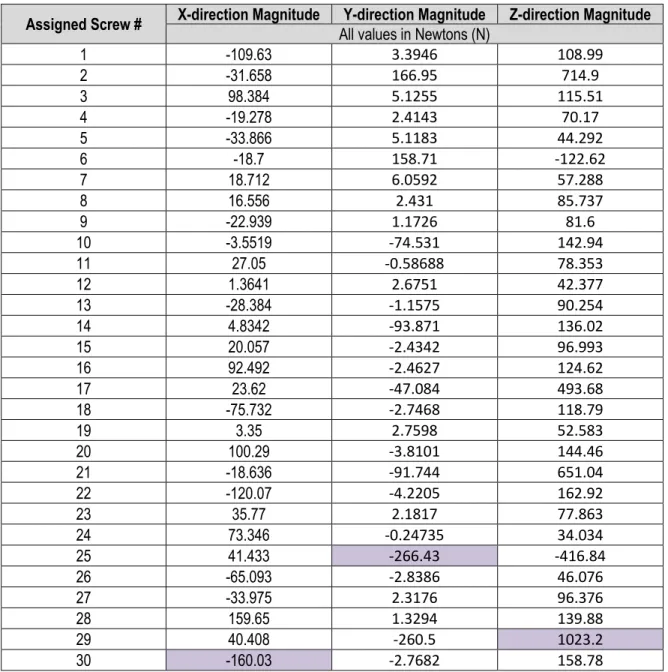
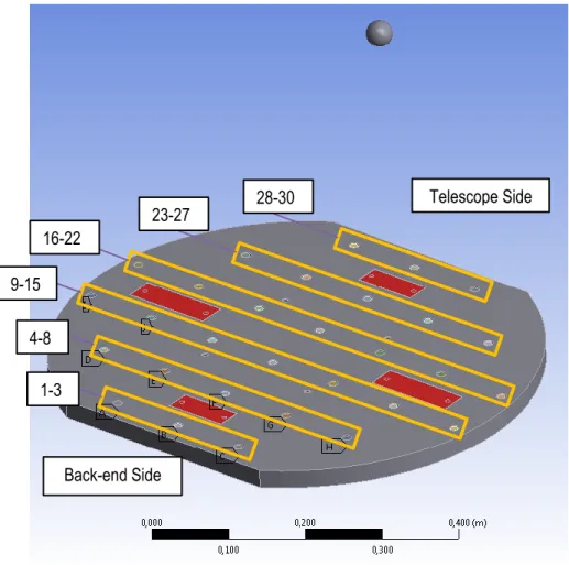
1.4.2.2.2 Interface Plate Screws – Force Analysis

The interface plate screws are the screws that fix the payload (using the interface place) to the gondola’s floor; there is a total of thirty M6 screws that are used for this as displayed in Figure 22. This section is relevant to improve the confidence in the load distribution across the gondola floor’s inserts and to prove conformance to Requirements 11-13. It was deemed important to analyze since the screws are experiencing increased loads from the acceleration of the entire mount structure and because the gondola floor’s inserts have never been subject to a payload of this size before.

Using the strategy and parameters mentioned in Section 2.4.2.1, the simulation was performed, and the results are shown in Table 4 with the maximum forces for each direction highlighted; for convenience, Figure 22 displays the interface plate simulation model with the assigned screws’ numbers.

Table 4: Force reactions for the screws interfacing the mount structure to the gondola’s floor

Assigned Screw # X-direction Magnitude _{All values in Newtons (N)}Y-direction Magnitude Z-direction Magnitude

1 -109.63 3.3946 108.99 2 -31.658 166.95 714.9 3 98.384 5.1255 115.51 4 -19.278 2.4143 70.17 5 -33.866 5.1183 44.292 6 -18.7 158.71 -122.62 7 18.712 6.0592 57.288 8 16.556 2.431 85.737 9 -22.939 1.1726 81.6 10 -3.5519 -74.531 142.94 11 27.05 -0.58688 78.353 12 1.3641 2.6751 42.377 13 -28.384 -1.1575 90.254 14 4.8342 -93.871 136.02 15 20.057 -2.4342 96.993 16 92.492 -2.4627 124.62 17 23.62 -47.084 493.68 18 -75.732 -2.7468 118.79 19 3.35 2.7598 52.583 20 100.29 -3.8101 144.46 21 -18.636 -91.744 651.04 22 -120.07 -4.2205 162.92 23 35.77 2.1817 77.863 24 73.346 -0.24735 34.034 25 41.433 -266.43 -416.84 26 -65.093 -2.8386 46.076 27 -33.975 2.3176 96.376 28 159.65 1.3294 139.88 29 40.408 -260.5 1023.2 30 -160.03 -2.7682 158.78

(35)

Figure 22: Interface plate with assigned numbering scheme for the insert screws

Application of standard safety factor to the maximum forces experienced in each direction:

𝑿 − 𝒅𝒊𝒓𝒆𝒄𝒕𝒊𝒐𝒏: 160.03 × 1.2 = 𝟏𝟗𝟐. 𝟎𝟒 𝑵 𝒀 − 𝒅𝒊𝒓𝒆𝒄𝒕𝒊𝒐𝒏: 266.43 × 1.2 = 𝟑𝟏𝟗. 𝟕𝟐 𝑵 𝒁 − 𝒅𝒊𝒓𝒆𝒄𝒕𝒊𝒐𝒏: 1023.2 × 1.2 = 𝟏𝟐𝟐𝟕. 𝟖𝟒 𝑵

In order to satisfy Requirements 11 and 12, we can compare these maximum forces experienced to the limits defined in the requirements themselves. The values, after applying a standard safety factor of 1.2, are less than the values provided by CNES for the requirements. Since the maximum forces in each direction across all the screws are all below the limits, it is implied that the forces on all the screws, in all directions, are also below the limits. Therefore, we can conclude that Requirements 11 and 12 are satisfied.

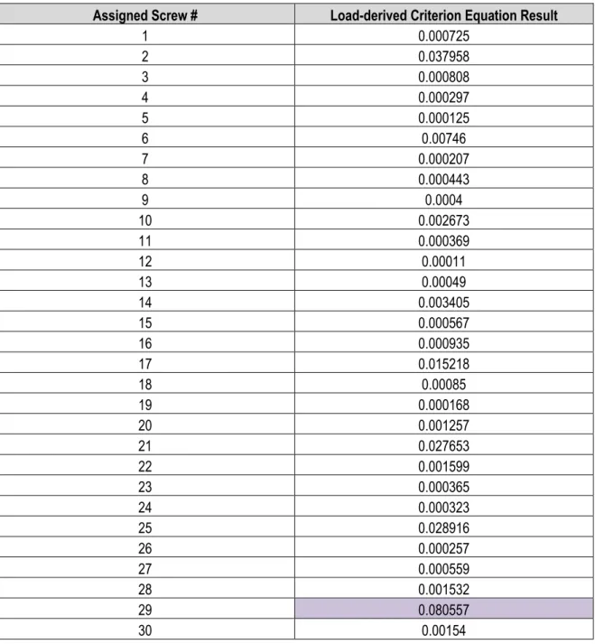
In order to satisfy Requirement 13, however, further calculations must be made. Table 5 outlines the results of calculations performed in Excel that uses the equation defined in Requirement 13 to see if the forces experienced by each screw satisfy the criterion. The maximum normal load (P) is taken as the Y-direction force reaction and the maximum transverse load (Q) is taken as the vector sum of the X- and Z-direction forces.

1-3 4-8 9-15 16-22 23-27 28-30 Telescope Side Back-end Side

(36)

Table 5: Verification of conformance of loads on each screw for the force equation criterion

Assigned Screw # Load-derived Criterion Equation Result

1 0.000725 2 0.037958 3 0.000808 4 0.000297 5 0.000125 6 0.00746 7 0.000207 8 0.000443 9 0.0004 10 0.002673 11 0.000369 12 0.00011 13 0.00049 14 0.003405 15 0.000567 16 0.000935 17 0.015218 18 0.00085 19 0.000168 20 0.001257 21 0.027653 22 0.001599 23 0.000365 24 0.000323 25 0.028916 26 0.000257 27 0.000559 28 0.001532 29 0.080557 30 0.00154

With the largest result being 0.080557, it’s clear that the criterion is met for all the screws. With this, we can conclude that the design satisfies Requirement 13 as well.

(37)

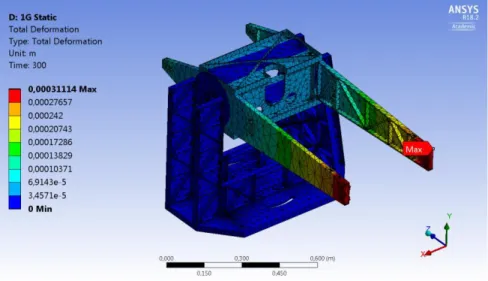
1.4.2.2.3 Full Structure (1G Static) – Stress Analysis

The top section and mid section of the mount design was analyzed separately for the worst-case impact load simulations because the interaction between the two can be difficult to model correctly. Separating them yields two simulations that are more accurate instead of a single inaccurate simulation resulting from a poorly constructed model. However, the full structure still requires a 1G static analysis. This analysis is important to assess how the mount structure behaves under its own weight while it is not moving. It is simulation that does not have a validation criterion, the main purpose is to find the critical areas in the design (the most stressed) and assess if the maximum stresses on those areas are reasonable.

Using the strategy and parameters mentioned in Section 2.4.2.1, the simulation was performed, and the results are shown in Figures 23 and 24.

Figure 23: Maximum Von-Mises stress from the 1G static simulation of the structure

(38)

The maximum stress from the 1G static test occurs on the shaft that connects the telescope arm to the coupling. This was expected since the shafts are supporting the weight of the entire top section of the mount. The stress induced by the weight of the mount is very low (18.4 MPa), though, and does not raise any concerns for failure under its own weight. This further lends to proving the structural integrity of the design.

The maximum deformation is more relevant for this simulation because it provides information that may directly affect the pointing system. A deformation of 0.311 mm can be observed at the ends of the telescope arms, which is very small compared to it’s overall length and does not present a problem for the pointing system that has an auto-adjustment feature within the algorithm.

1.4.2.3 Verification and Validation (V&V) of Results

This section will demonstrate the measures taken post-simulation to build confidence in the simulation results.

There are numerous ways to check the validity of simulation results within ANSYS. For this simulation, 3 verification checks were performed: convergence, structural error, and mesh quality. All of these are, essentially, providing you with the same information (the accuracy of your results), but they confirm it in different ways and with different metrics.

The first check to perform is the convergence check. This is a broad scope check that provides information on how well the numerical solver was able to work through the finite element calculations. This is done by establishing a validation criterion by setting a predefined level of permissible error for the change in

stress across elements and between timesteps. Typically, an error of 10-20% is acceptable for most applications;

10% was chosen for this simulation to be safe. ANSYS is then able to generate a convergence curve based on the numerical solver’s ability to find an accurate solution. Whenever it can converge to an acceptable solution (in the acceptable amount of iterations), the curve should be below the curve of the validation criterion. This check was performed for all the simulations; the result for the standing structures simulation is displayed in Figure 25 with the criterion curve in blue and the convergence curve in purple.

(39)

Figure 25: Stress convergence curve for the full-assembly structural simulation

The convergence curve is below the validation criterion curve for almost the entire duration of the simulation, which is a good indication that the next checks should yield positive results as well. If convergence problems were present, the next checks would be used to investigate the specific problem areas and find solutions accordingly; typically, the solution can be resolved by refining the mesh or changing element geometry in those problem areas.

The second check is the structural error check. This check is excellent for indicating the areas in the simulation model that require mesh refinement because of problems in the finite element calculations in those areas. It is, essentially, a more in-depth version of the convergence check. If specific areas, or even specific elements, are causing problems, it will take longer to converge, or will not converge at all and the structural error is able to display this. There were many problem areas with the original simulation models because of the bracketed design’s curves. The mesh was refined in these areas and some elements were merged with adjacent elements to avoid the overlap of element areas. Across all simulations, a maximum structural error of 0.072 (7.2%) was achieved, which is within the accepted range (up to 10%) defined by ANSYS.

Lastly is the mesh quality check using the aspect ratio and element quality as metrics. The aspect ratio defines the degree to which elements are “stretched” in the mesh generation to fill out the simulation model; in other words. This can impact the simulation results because a large aspect ratio could cause mesh elements to span a large area in one direction. This can yield inaccurate results and impact the rest of the results in the numerical solver that follow that element’s location. Typically, aspect ratio values under 10 is excellent, with larger aspect ratios (around 20) being accepted for elements outside the critical areas if they make up less than

(40)

10% of the total elements. Figure 26 demonstrates the distribution of the aspect ratios for the standing structures simulation model used.

Figure 26: Distribution of aspect ratios of the standing structures simulation model

As observed, the aspect ratio of all the elements are below 10, indicating a great consistency in the shape of the elements. This check can be considered a success since it follows the criteria mentioned earlier.

Element quality is a more encompassing metric that is based on a ratio of the volume to the edge length. More specifically, it is determined by the following equation:

𝐸𝑙𝑒𝑚𝑒𝑛𝑡 𝑄𝑢𝑎𝑙𝑖𝑡𝑦 = 𝑆ℎ𝑎𝑝𝑒 𝐹𝑎𝑐𝑡𝑜𝑟 × 𝑉𝑜𝑙𝑢𝑚𝑒

√[∑(𝐸𝑑𝑔𝑒 𝐿𝑒𝑛𝑔𝑡ℎ)2_]3

This is a check that is comparable to the aspect ratio in that it aims to check how stretched out the elements are. A value of 1 would imply that the element is a perfect cube, whereas a value close to zero would imply a shape that is flatter with some edge lengths much longer than others. This being the case, in order to have a good balance of edge lengths, an element quality larger than 0.30 is required. Figure 27 demonstrates the distribution of the element quality for all elements for the standing structures simulation model used.

(41)

Figure 27: Distribution of element quality for the standing structures simulation model

As observed, the element quality of all the elements are above 0.30, which is also indicative of great geometry of the elements. This check can be considered a success since it also follows the criteria mentioned earlier.

(42)

1.4.2.4 Summary of Results

1.4.2.4.1 Numerical Analyses

Table 6: Summary of numerical results for the standing mount structure

Area Stress Type Analysis _Result _PermissibleMax Factor of _Safety Conform?

RM-3 Motor

Normal Load (N) Negligible 200.12 N/A N/A

Moment Load (N·m) 0.4188 13.5 32.23 Y

Torque (N·m) Negligible 4.50 N/A N/A

RM-8 Motor

Normal Load (N) 698.6 3 109.77 4.451 Y

Moment Load (N·m) 105.29 135.50 1.287 Y

Torque (N·m) Negligible 23 N/A N/A

Altitude-Direction

Coupling Torque (N·m) 8.094 10 1.235 Y

1.4.2.4.2 Simulation Analyses

Table 7: Summary of simulation results for the standing mount structure

Area Stress Type Indicator Sim. Result Max Permissible Conform?

Telescope Arm Structure Von-Mises (MPa) DYL 133.31 276 Y DUL 159.98 310 Y

Telescope Screws N/A 11.712 1172.11 Y

Standing Structures (Mid-Portion)

DYL 221.45 276 Y

DUL 265.74 310 Y

Full Structure N/A 18.40 N/A N/A

Interface Screws Force (N) Max X-Z 1035.7 4080 Y

(43)

1.4.3 Mission Performance

Although there aren’t many quantitative means to measure the performance of the telescope mount, there is still room for discussion. This section will highlight specific subjects surrounding the telescope mount, provide more information about how they performed, and the problems encountered.

1.4.3.1 Structural Integrity

Based on inspection post-flight, the large structures proved to be well-designed. There was no major structural damage done to the mount itself, all parts could be reused for future missions, if desired. There are countless 1-mm diameter dents throughout the structure caused by the jettisoned stainless-steel balls used for altitude control, but it’s not enough to impact the structural integrity of the design in a significant manner. For context, Figure 28 displays the type of landing environment that the payload landed in and withstood.

Figure 28: Landing environment of the gondola

The only data we have that can be used to measure the performance of the structure is the acceleration loads that were experienced by the gondola during the major events. CNES provided this data and the full graphs are available in Appendix 4; for convenience, however, Table 8 summarizes the maximum loads experienced at separation and at landing, along with the loads that the mount was designed to withstand for each.