O
pen
A
rchive
T
OULOUSE
A
rchive
O
uverte (
OATAO
)
OATAO is an open access repository that collects the work of Toulouse researchers and
makes it freely available over the web where possible.
This is an author-deposited version published in :
http://oatao.univ-toulouse.fr/
Eprints ID : 12968
To link to this article :
DOI:10.1109/TMI.2012.2225636
URL :
http://dx.doi.org/10.1109/TMI.2012.2225636
To cite this version :
Chaari, Lotfi and Vincent, Thomas and Forbes, Florence
and Dojat, Michel and Ciuciu, Philippe Fast joint detection-estimation of
evoked brain activity in event-related fmri using a variational approach.
(2013) IEEE Transactions on Medical Imaging, vol. 32 (n° 5). pp. 821-837.
ISSN 0278-0062
Any correspondance concerning this service should be sent to the repository
administrator: [email protected]
Fast Joint Detection-Estimation of Evoked
Brain Activity in Event-Related fMRI
Using a Variational Approach
LotÞ Chaari*, Member, IEEE, Thomas Vincent, Florence Forbes, Michel Dojat, Senior Member, IEEE, and
Philippe Ciuciu, Senior Member, IEEE
Abstract—In standard within-subject analyses of event-related functional magnetic resonance imaging (fMRI) data, two steps are usually performed separately: detection of brain activity and estimation of the hemodynamic response. Because these two steps are inherently linked, we adopt the so-called region-based joint detection-estimation (JDE) framework that addresses this joint issue using a multivariate inference for detection and estimation. JDE is built by making use of a regional bilinear generative model of the BOLD response and constraining the parameter estimation by physiological priors using temporal and spatial information in a Markovian model. In contrast to previous works that use Markov Chain Monte Carlo (MCMC) techniques to sample the resulting intractable posterior distribution, we recast the JDE into a missing data framework and derive a variational expectation-maximization (VEM) algorithm for its inference. A variational approximation is used to approximate the Markovian model in the unsupervised spatially adaptive JDE inference, which allows automatic Þne-tuning of spatial regularization parameters. It provides a new algorithm that exhibits interesting properties in terms of estimation error and computational cost compared to the previously used MCMC-based approach. Experiments on artiÞcial and real data show that VEM-JDE is robust to model misspeciÞcation and provides computational gain while main-taining good performance in terms of activation detection and hemodynamic shape recovery.
Index Terms—Expectation-maximization (EM) algorithm, func-tional magnetic resonance imaging (fMRI), joint detection-estima-tion, Markov random Þeld, variational approximation.
Manuscript received July 23, 2012; revised October 01, 2012; accepted Oc-tober 09, 2012. Date of publication OcOc-tober 19, 2012; date of current version April 27, 2013. Asterisk indicates corresponding author.
*L. Chaari is with the Mistis team, Inria Grenoble Rhône-Alpes, 38334 Saint Ismier Cedex, France, and also with the University Joseph Fourier, 38041 Grenoble, France, and also with the CEA/DSV/I2BM/Neurospin, CEA Saclay, 91191 Gif-sur-Yvette cedex, France (e-mail: lotÞ[email protected]).
T. Vincent is with the Mistis team, Inria Grenoble Rhône-Alpes, 38334 Saint Ismier Cedex, France, and also with the University Joseph Fourier, 38041 Grenoble, France, and also with the CEA/DSV/I2BM/Neurospin, CEA Saclay, 91191 Gif-sur-Yvette cedex, France (e-mail: [email protected]).
F. Forbes is with the Mistis team, Inria Grenoble Rhône-Alpes, 38334 Saint Ismier Cedex, France, and also with the University Joseph Fourier, 38041 Grenoble, France.
M. Dojat is with INSERM, U836, GIN and University Joseph Fourier, 38041 Grenoble, France (e-mail: [email protected]).
P. Ciuciu is with CEA/DSV/I2BM/Neurospin, CEA Saclay, 91191 Gif-sur-Yvette cedex, France (e-mail: [email protected]).
Color versions of one or more of the Þgures in this paper are available online at http://ieeexplore.ieee.org.
Digital Object IdentiÞer 10.1109/TMI.2012.2225636
I. INTRODUCTION
F
UNCTIONAL magnetic resonance imaging (fMRI) is a powerful tool to noninvasively study the relationship between a sensory or cognitive task and the ensuing evoked neural activity through the neurovascularcoupling measured by the BOLD signal [1]. Since the 1990s, this neuroimaging modality has become widely used in brain mapping as well as in functional connectivity study in order to probe the spe-cialization and integration processes in sensory, motor, and cognitive brain regions [2]–[4]. In this work, we focus on the recovery of localization and dynamics of local evoked activity, thus on specialized cerebral processes. In this setting, the key issue is the modeling of the link between stimulation events and the induced BOLD effect throughout the brain. Physiological nonlinear models [5]–[8] are the most speciÞc approaches to properly describe this link but their computational cost and their identiÞability issues limit their use to a restricted number of speciÞc regions and to a few experimental conditions. In contrast, the common approach, being the focus of this paper, rather relies on linear systems which appear more robust and tractable [2], [9]. Here, the link between stimulation and BOLD effect is modelled through a convolutive system where each stimulus event induces a BOLD response, via the convolution of the binary stimulus sequence with the hemodynamic re-sponse function (HRF). There are two goals for such BOLD analysis: the detection of where cerebral activity occurs and the estimation of its dynamics through the HRF identiÞca-tion. Commonly, the estimation part is ignored and the HRF is Þxed to a canonical shape which has been derived from human primary visual area BOLD response [10], [11]. The detection task is performed by a general linear model (GLM), where stimulus-induced components are assumed to be known and only their relative weighting are to be recovered in the form of effect maps [2]. However, spatial intra-subject and between-subject variability of the HRF has been highlighted [12]–[14], in addition to potential timing ßuctuations induced by the paradigm (e.g., variations in delay [15]). To take this variability into account, more ßexibility can be injected in the GLM framework by adding more regressors. In a parametric setting, this amounts to adding a function basis, such as canon-ical HRF derivatives, a set of gamma or logistic functions [15], [16]. In a nonparametric setting, all HRF coefÞcients are explicitly encoded as a Þnite impulse response (FIR) [17]. The major drawback of these GLM extensions is the multiplicity of regressors for a given condition, so that the detection taskbecomes more difÞcult to perform and that statistical power is decreased. Moreover, the more coefÞcients to recover, the more ill-posed the problem becomes. The alternative approaches that aim at keeping a single regressor per condition and add also a temporal regularization constraint to Þx the ill-posedness are the so-called regularized FIR methods [18]–[20]. Still, they do not overcome the low signal-to-noise ratio (SNR) inherent to BOLD signals, and they lack robustness especially in nonac-tivated regions. All the issues encountered in the previously mentioned approaches are linked to the sequential treatment of the detection and estimation tasks. Indeed, these two problems are strongly linked: on the one hand, a precise localization of brain activated areas strongly depends on a reliable HRF model; on the other hand, a robust estimation of the HRF is only possible in activated areas where enough relevant signal is measured [21]. This interdependence and retroactivity has motivated the idea to jointly perform these two tasks [22]–[24] (detection and estimation) in a joint detection-estimation (JDE) framework [25] which is the basis of the approach developed in this paper. To improve the estimation robustness, a gain in HRF reproducibility is performed by spatially aggregating signals so that a constant HRF shape is locally considered across a small group of voxels, i.e., a region or a parcel. The procedure then implies a partitioning of the data into functionally homoge-neous parcels, in the form of a cerebral parcellation [26]. As will be recalled in more detail in Section II, the JDE approach rests upon three main elements: 1) a nonparametric or FIR parcel-level modeling of the HRF shape; 2) prior information about the temporal smoothness of the HRF to guarantee its physiologically plausible shape; and 3) the modeling of spatial correlation between the response magnitudes of neighboring voxels within each parcel using condition-speciÞc discrete hidden Markov Þelds. In [22], [23], [25], posterior inference is carried out in a Bayesian setting using a computationally intensive Markov Chain Monte Carlo (MCMC) method, which is computationally intensive and requires Þne tuning of several parameters.
In this paper, we reformulate the complete JDE framework [25] as a missing data problem and propose a simpliÞcation of its estimation procedure. We resort to a variational approx-imation using a variational expectation maximization (VEM) algorithm in order to derive estimates of the HRF and stim-ulus-related activity. Variational approximations have been widely and successfully employed in the context of fMRI data analysis: 1) to model auto-regressive noise in the context of a Bayesian GLM [27]; 2) to characterize cerebral hierarchical dynamic models [28]; 3) to model transient neuronal signals in a Bayesian dynamical system [29] or 4) to perform inference of spatial mixture models for the segmentation of GLM effect maps [30]. As in our study, the primary goal of resorting to variational approximations is to alleviate the computational burden associated with stochastic MCMC approaches. Akin to [30], we aim at comparing the stochastic and variational-based inference schemes, but on the more complex matter of detecting activation and estimating the HRF whereas [30] treated only a detection problem.
Compared to the JDE MCMC implementation, the proposed approach does not require priors on the model parameters for
TABLE I
ACRONYMSUSED IN THEJDE MODELPRESENTATION ANDINFERENCE
inference to be carried out. However, such priors may be in-jected in the adopted model for more robustness and to make the proposed approach fully auto-calibrated. Experiments on artiÞcial and real data demonstrate the good performance of our VEM algorithm. Compared to the MCMC implementation, VEM is more computationally efÞcient, robust to misspeciÞca-tion of the parameters, to deviamisspeciÞca-tions from the model, and adapt-able to various experimental conditions. This increases consid-erably the potential impact of the JDE framework and makes its application to fMRI studies in cognitive and clinical neuro-science easier and more valuable. This new framework has also the advantage of providing straightforward criteria for model selection.
The rest of this paper is organized as follows. In Section II, we introduce the hierarchical Bayesian model for the JDE frame-work in the within-subject fMRI context. In Section III, the VEM algorithm based on variational approximations for infer-ence is described. Evaluation on real and artiÞcial fMRI datasets are reported in Section IV and the performance comparison be-tween the MCMC and VEM implementations is carried out in Section V. Finally, Section VI discusses the pros and cons of the proposed approach and some perspectives.
II. BAYESIAN FRAMEWORK FOR THE JOINT
DETECTION-ESTIMATION
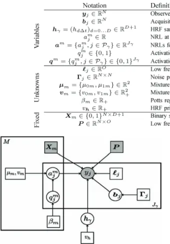
Matrices and vectors are denoted with bold upper and lower case letters (e.g., and ). A vector is by convention a column vector. The transpose is denoted by . Unless stated otherwise, subscripts , , and are respectively indexes over voxels, stimulus types, mixture components, and time points. The Gaussian distribution with mean and covariance matrix is denoted by . The main acronyms used in the paper are deÞned in Table I. Table II gathers deÞnitions of the main variables and parameters. A graphical representation of the model is given in Fig. 1.
A. The Parcel-Based Model
We Þrst recast the parcel-based JDE model proposed in [23], [25] in a missing data framework. Let us assume that the brain is decomposed in parcels, each of them con-taining voxels and having homogeneous hemodynamic prop-erties. The fMRI time series is measured in voxel at times , where , being the number of
TABLE II
NOTATIONS FORVARIABLES ANDPARAMETERSUSED IN THEMODEL FOR AGIVENPARCEL WITH VOXELS
Fig. 1. Graphical model describing dependencies between latent and observed variables involved in the JDE generative model for a given parcel with voxels. Circles and squares indicate random variables and model parameters, re-spectively. Observed variables and Þxed parameters are shaded. We used stan-dard graphical notations where plates represent multiple similar nodes with their number given in the plate.
scans and , the time of repetition. The number of different stimulus types or experimental conditions is . For a given parcel containing a group of connected voxels, a unique BOLD signal model is used in order to link the observed data
to the unknown HRF
speciÞc to , and also to the unknown response amplitudes with , being the magnitude at voxel for condition . More speciÞcally, the observation model at each voxel is expressed as follows [23]:
(1)
where is the summation of the stimulus-induced components of the BOLD signal. The binary matrix is of size and provides information on the stim-ulus occurrences for the th experimental condition, being the sampling period of the unknown HRF in . This hemodynamic response is a consequence of the neuronal excitation which is commonly assumed to occur following stimulation. The scalars ’s are
weights that model the response magnitude evoked by the stimuli, whose occurrences are informed by the matrices . They model the transition between stimuli and the vascular response informed by the Þlter . It follows that the ’s are generally referred to as neural response levels (NRLs). The rest of the signal is made of matrix , which corresponds to physiological artifacts accounted for via a low frequency orthonormal function basis of size . With each voxel is associated a vector of low frequency drifts
which has to be estimated. Within parcel , these vectors may be grouped into the same matrix . As regards observation noise, the ’s are assumed to be independent with at voxel (see Section II-B-1 for more details). The set of all unknown precision matrices (inverse of the covariance matrices) is denoted by . The forward BOLD model expressed in (1) relies on the classical assumption of a linear and time invariant system which is adopted in the GLM framework [2]. Indeed, it can easily be recast in the same formulation where the response magnitudes ’s and drift coefÞcient ’s are equivalent to the effects associated with stimulus-induced and low frequency basis regressors, respectively. However, the JDE forward model generalizes the GLM model since the hemodynamics Þlter is unknown. Finally, detection is handled through the introduction of activation class assignments where and represents the activation class at voxel for condition . The NRL coefÞcients will therefore be expressed conditionally to these hidden variables. In other words, the NRL coefÞcients will depend on the activation status of the voxel , which itself depends on the activation status of neighboring voxels thanks to a Markov model used as a spatial prior on (cf Section II-B2c). Without loss of generality, we consider here two activation classes akin to [25] (activated and nonactivated voxels). An additional deactivation class may be considered depending on the experiment as proposed within the JDE context in [31]. In the following developments, all provided formulas are general enough to cover this case.
B. A Hierarchical Bayesian Model
In a Bayesian framework, we Þrst need to deÞne the likelihood and prior distributions for the model
vari-ables and parameters . Using the hi-erarchical structure between , , , , and , the complete model is given by the joint distribution of both the observed and unobserved (or missing) data: . To fully deÞne the hierarchical model, we now specify each term.
1) Likelihood: The deÞnition of the likelihood depends on
the noise model assumptions. In [23], [32], an autoregressive (AR) noise model has been adopted to account for serial corre-lations in fMRI time series. It has also been shown in [23] that a spatially-varying Þrst-order AR noise model helps control the false positive rate. In the same context, we will assume such a noise model with where is a tridiagonal symmetric matrix which depends on the AR(1)
pa-rameter [23]: , for
and for
. These parameters are assumed voxel-speciÞc due to their tissue-dependence [33], [34]. Denoting
and , the likelihood can be factorized over voxels as follows:
(2)
2) Model Priors:
a) Hemodynamic response function: Akin to [23], [25], we
introduce constraints in the HRF prior that favor smooth vari-ations in by controlling its second order derivative:
with where is the second-order Þnite difference matrix and is a parameter to be esti-mated. Moreover, boundary constraints have also been Þxed on as in [23], [25] so that . The prior assumption expressed on the HRF amounts to a smooth FIR model intro-duced in [18] and is ßexible enough to recover any HRF shape.
b) Neural response levels: Akin to [23], [25], the NRLs
are assumed to be statistically independent across
condi-tions: where
and gathers the parameters for the th condition. A mixture model is then adopted by using the assignment vari-ables to segregate nonactivated voxels from acti-vated ones . For the th condition, and conditionally to the assignment variables , the NRLs are assumed to be
in-dependent: . If
then . It is worth noting that the Gaussianity assumed for a given NRL is similar to the assumption of Gaussian effects in the classical GLM context [10]. The Gaussian parameters are unknown. For the sake of conciseness, we rewrite
where with and
with . More specif-ically, for nonactivated voxels we set for all , .
c) Activation classes: As in [25], we assume prior
independence between the experimental conditions re-garding the activation class assignments. It follows that where we assume in addition that
is a Markov random Þeld prior, namely a Potts model. Such prior modeling assumption is consistent with the physiological properties of the fMRI signal where the activity is known to be correlated in space [33], [35]. Here, the prior Potts model with interaction parameter [25] is expressed as
(3)
and where is the normalizing constant and for all if and 0 otherwise. The notation means that the summation is over all neighboring voxels. The unknown parameters are denoted by . In what follows, we will consider a six-connexity 3-D neighboring system.
For the complete model, the whole set of parameters is de-noted by and belong to a set .
III. ESTIMATION BY VARIATIONAL
EXPECTATION-MAXIMIZATION
We propose to use an expectation-maximization (EM) frame-work to deal with the missing data namely, , ,
.
A. Variational Expectation-Maximization Principle
Let be the set of all probability distributions on . EM can be viewed [36] as an alternating maximization proce-dure of a function on , for all
(4) where denotes the expectation with respect to and is the entropy of . This function is called the free energy functional. It can be equivalently expressed in terms of the log-likelihood as where is the KL divergence between and
(5)
Hence. maximizing the free energy with respect to amounts to minimizing the KL divergence between and the posterior dis-tribution of interest . Since the KL divergence is always non-negative, and because the KL divergence of the posterior distribution to itself is zero, it follows easily that the maximum free energy over all is the log-likelihood. The link to the EM algorithm follows straightforwardly. At iteration , denoting the current parameter values by , the alter-nating procedure proceeds as follows:
(6)
However, the optimization step in (6) leads to
, which is intractable for our model. Hence, we resort to a variational EM (VEM) variant in which the intractable posterior is approximated by constraining the space of possible distributions in order to make the maximiza-tion procedure tractable. In that case, the free energy optimal value reached is only a lower bound on the log-likelihood. The most common variational approximation consists of optimizing over the distributions in that factorize as a product of three pdfs on , and , respectively.
Previous attempts to use variational inference [37], [38] and in particular in fMRI [27], [30] have been successful, with this type of approximations usually validated by assessing its Þdelity to its MCMC counterpart. In Section IV, we will also provide such a comparison. The actual consequences of the factorization may vary with the models under study. Some couples of latent variables may capture more dependencies that would then need to be kept whereas others may induce only weak local corre-lation at the expense of a long-range correcorre-lation which to Þrst order can be ignored (see [39] for more details on the conse-quences of the factorization for particular models). The way it may affect inference is that often variational approximations are shown to lead to underestimated variances and consequently to conÞdence intervals that are too narrow. Note that [38] sug-gested that nonparametric bootstrap intervals whenever possible may alleviate this issue. Also, when the concern is the compu-tation of maximum a posteriori estimates, the required ingre-dients for designing an accurate variational approximation lie in the shape of the optimized free energy. All that is needed for our inference to work well is that the optimized free energy have a similar shape (mode and curvature) to the target log-like-lihood whenever the likelog-like-lihood is relatively large. As a matter of fact, there are cases, such as mixtures of distributions from the exponential family, where the variational estimator is asymp-totically consistent. The experiments in [38] even report very accurate conÞdence intervals. Unfortunately no general theo-retical results exist that would include our case to guarantee the accuracy of estimates based on the variational approxima-tion. The other few cases for which the variational approach has shown good theoretical properties are to the best of our knowl-edge simpler than our setting. The fact that the HRF can be equivalently considered as a missing variable or a random pa-rameter induces some similarity between our VEM variant and the Variational Bayesian EM algorithm in [37]. Our framework varies slightly from the case of conjugate exponential models described in [37] and more importantly, our presentation offers the possibility to deal with extra parameters for which prior information may not be available. This is done in a maximum likelihood manner and avoids tusing noninformative priors that could be problematic [40, pp. 64–65]. Consequently, the vari-ational Bayesian M-step of [37] is transferred into our E-step while our M-step has no equivalent in the formulation of [37].
B. Variational Joint Detection-Estimation
We propose here to use a EM variant in which the intractable E-step is instead solved over , a restricted class of probability distributions chosen as the set of distributions that factorize as
where , and are probability distributions on , and , respectively. It follows then that our E-step becomes an approximate E-step, which can be further decomposed into three stages that consist of updating the three pdfs, , and in turn using three equivalent expressions of when factorizes as in . At iteration with current es-timates denoted by , and , the up-dating rules become
In other words, the factorization is used to maximize the free energy by alternately maximizing it with respect to , and while keeping the other distributions Þxed. The steps above can then be equivalently written in terms of minimizations of some KL divergences. The properties of the latter lead to the following solutions (see Appendix for details):
(8)
(9)
(10)
The corresponding is (since and are independent [see (4)]
(11) These steps lead to explicit calculations for , , and the parameter set . Although the approximation by a factorized distribution may have seemed initially drastic, the equations it leads to are cou-pled. More speciÞcally, the approximation consists of replacing stochastic dependencies between latent variables by determin-istic dependencies between moments of these variables (see Appendices A to C as mentioned below).
• step: From (8) standard algebra enables to derive that is a Gaussian distribution
whose parameters are detailed in Appendix B. The expres-sions for and are similar to those derived in the MCMC case [23, Eq. (B.1)] with expressions involving the ’s replaced by their expectations with respect to with re-spect to .
• step: Using (9), standard algebra rules allow to identify the Gaussian distribution of which writes as with . More de-tail about the update of is given in Appendix C. The relationship with the MCMC update of is not straight-forward. In [23], [25], the ’s are sampled independently and conditionally on the ’s. This is not the case in the VEM framework but some similarity appears if we set the probabilities either to 0 or 1 and consider only the diagonal part of .
• step: Using the expressions of and in Section II, (10) yields
which is intractable due to the Markov random Þeld prior. To overcome this difÞculty, a number of ap-proximation techniques are available. To decrease the computational complexity of our VEM algorithm and to avoid introducing additional variables as done in [30], we use a mean-Þeld like algorithm which con-sists of Þxing the neighbors to their mean value. Fol-lowing [41], can be approximated by a fac-torized density such that if ,
where is a par-ticular conÞguration of updated at each itera-tion according to a speciÞc scheme, denotes neighboring voxels to on the brain volume and
. Hereabove, and
denote the and entries of the mean vector and covariance matrix , respectively. The Gaussian distribution with mean and variance is denoted by , while . More details are given in Appendix D.
• step: For this maximization step, we can Þrst rewrite (11) as
(12)
The M-step can therefore be decoupled into four sub-steps involving separately , , and . Some of these sub-steps admit closed-form expressions, while some other require resorting to iterative or alternate optimiza-tion. For more details about the related calculations, the interested reader can refer to Appendix E.
IV. VALIDATION OF THEPROPOSEDAPPROACH
This section aims at validating the proposed variational ap-proach. Synthetic and real contexts are considered respectively in Sections IV-A and IV-B. To corroborate the effectiveness of the proposed method, comparisons with its MCMC counterpart, as implemented in [25], will also be conducted throughout the
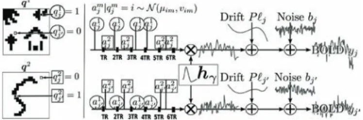
Fig. 2. Single parcel artiÞcial data generation process using two experi-mental conditions . From left to right: label maps are hand-drawn. Conditionally on them, NRL values are drawn from Gaussian distributions with means and variances whenever . Then, for any given voxel , the stimulus sequence of a given experimental condition is multiplied by the corresponding NRL value . The resulting sequence is convolved with a normalized HRF which is common to all conditions and voxels. Nuisance signals are Þnally added (drift and noise ) to form the artiÞcial BOLD signal .
present section. The two approaches have been tuned at best so as to make them as close as possible. This reduces essentially to moderate the effect of the MCMC priors. The hyper-priors have been parameterized by a set of hyper-parameters that have a lim-ited impact on the priors themselves. For instance, for the mean and variance parameters involved in the mixture model , conjugate Gaussian and inverse-gamma
hyper-prior distributions have been considered whose param-eters have been tuned by hand so as to make them ßat while proper (e.g., ). For doing so, the relationship between the hyper-parameters (e.g., ) and the statistical moments of the distribution have been carefully studied to guarantee a large variance or a large entropy in the latter. Moreover, given the above mentioned ßatness of the hyper-priors, the MCMC approach is fairly robust to hyper-parameter setting.
A. ArtiÞcial fMRI Datasets
In this section, experiments have been conducted on data sim-ulated according to the observation model in (1) where has been deÞned from a cosine transform basis as in [23]. The sim-ulation process is illustrated in Fig. 2.
Different studies have then been conducted in order to vali-date the detection-estimation performance and robustness. For each of these studies, some simulation parameters have been changed such as the noise or the paradigm properties. Changing these parameters aims at providing for each simulation context a realistic BOLD signal while exploring various situations in terms of SNR.
1) Detection-Estimation Performance: The Þrst
artiÞ-cial data analysis was conducted on data simulated with a Gaussian white noise ( is the -di-mensional identity matrix). Two experimental conditions have been considered while ensuring stim-ulus-varying contrast-to-noise ratios (for condition , ) achieved by setting , , , and , so that a higher CNR is simu-lated for the Þrst experimental condition
compared to the second one . For each of these conditions, the initial artiÞcial paradigm comprised 30 stimulus events. The simulation process Þnally yielded time-series of 268 time-points. Condition-speciÞc activated
Fig. 3. Detection results for the Þrst artiÞcial data analysis. Ground truth (left) and estimated PPM using MCMC (middle) and VEM (right). Note that condition (bottom row) is associated with a lower CNR than condition
(top row).
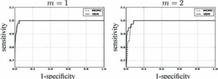
Fig. 4. Detection results for the Þrst artiÞcial data analysis. ROC curves associ-ated with the label posteriors using VEM and MCMC. Condition is associated with a higher CNR than condition . Curves are plotted in solid and dashed line for VEM and MCMC, respectively.
and nonactivated voxels ( values) were deÞned on a 20 20 2-D slice as shown in Fig. 2 [left]. No parcellation was per-formed. Simulated NRLs and BOLD signal were thus assumed to belong to a single parcel of size 20 20.
The posterior probability maps (PPMs) obtained using MCMC and VEM are shown in Fig. 3 [middle] and Fig. 3 [right]. PPMs here correspond to the activation class assign-ment probabilities . These Þgures clearly show the gain in robustness provided by the variational approx-imation. This gain consists of lower missclassiÞcation error (a lower false positive rate) illustrated by higher PPM values, especially for the experimental condition with the lowest CNR
.
For a quantitative evaluation, the receiver operating char-acteristic (ROC) curves corresponding to the estimated PPMs using both algorithms were computed. As shown in Fig. 4, they conÞrm that both algorithms perform well at high CNR
and that the VEM scheme outperforms the MCMC implemen-tation of the second experimental condition .
Fig. 5 shows the NRL estimates obtained by the two methods. Although some differences are exhibited on the PPMs, both al-gorithms report similar qualitative results with respect to the NRLs. However, the difference between NRL estimates (VEM-MCMC) in Fig. 5 [right] points out that regions corresponding to activated areas for the two conditions present positive inten-sity values, which means that VEM helps retrieving higher NRL values for activated area compared to MCMC.
Fig. 5. Detection results for the Þrst artiÞcial data analysis. From left to right: Ground truth and NRL estimates by MCMC and VEM, and NRL image difference (right). Top row: ; bottom row: .
Quantitatively speaking, the gain in robustness is con-Þrmed by reporting the sum of squared error
values on NRL estimates which are slightly lower using VEM compared to MCMC for the Þrst experimental condition ( : versus ), as well as for the second experimental
con-dition ( : versus ).
These error values indicate that, even though the MCMC algo-rithm gives the most precise PPMs for the high CNR condition (Fig. 4, ), the VEM approach is more robust than its MCMC alternative in terms of estimated NRLs. These values also indicate slightly lower SSE for the second experimental conditions compared to the Þrst one with higher CNR. This difference is explained by the presence of larger nonactivated areas for where low NRL values are simulated, and for which SSE is very low.
In addition, a test for equality of means has been conducted to test whether the quadratic errors means over voxels obtained with VEM and MCMC were signiÞcantly close. Very low p-values of 0.0377 and 0.0015 were obtained respectively for condition and , which means that the null hypothesis (the two means are equal) is rejected for the usual 5% threshold. In other words, although the obtained error difference is small, it is signiÞcant from a statistical viewpoint. Interestingly, As corresponds to a lower CNR, this highlights the signiÞcance of the gain in robustness we got with the VEM version in a degraded CNR context.
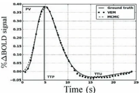
As regards HRF estimates, Fig. 6 shows both retrieved shapes using MCMC and VEM. Compared to the ground truth (solid line), the two approaches yield very similar results and preserve the most important features of the original HRF like the peak value (PV), time-to-peak (TTP), and time-to-undershoot (TTU).
2) Estimation Robustness: Since estimation errors may be
caused by different perturbation sources, in the following, var-ious Monte Carlo analyses have been conducted by varying one-at-a time several simulation parameters, namely the stim-ulus density, the noise parameters and the amount of spatial regularization. The differences in the obtained estimation errors have all been tested for statistical signiÞcance using tests for equality of means for the errors over 100 runs. For all reported comparisons, the obtained p-values were very low
indicating that the performance differences, even when small, were statistically signiÞcant.
Fig. 6. Estimation results for the Þrst artiÞcial data analysis. Ground truth HRF and HRF estimates using the MCMC and VEM algorithms.
a) Varying the stimulus density: In this experiment,
sim-ulations have been conducted by varying the stimulus density from 5 to 30 stimuli in the artiÞcial paradigm, which leads to decreasing interstimuli intervals (ISIs) (from 47 to 9 s, respec-tively). At each stimulus density, 100 realizations of the same ar-tiÞcial dataset have been generated so as to evaluate the estima-tion bias and variance of NRLs. Here, the stimuli are interleaved between the two conditions so that the above mentioned ISIs correspond to the time interval between two events irrespective of the condition they belong to. A second-order autoregressive noise (AR(2)) has also been used for the simulation providing a more realistic BOLD signal [23]. The rest of the simulation process is speciÞed as before. In order to quantitatively eval-uate the robustness of the proposed VEM approach to varying
input SNR ,
re-sults (assuming white noise in the model used for estimation for both algorithms) are compared while varying the stimula-tion rate during the BOLD signal acquisistimula-tion. Fig. 7 illustrates the error evolution related to the NRL estimates for both ex-perimental conditions with respect to the ISI (or equivalently the stimulus density) in the experimental paradigm. Estima-tion error is illustrated in terms of mean squared error (MSE) , which splits into the sum of the variance (Fig. 7 [top]) and squared bias (Fig. 7 [bottom]). This Þgure shows that at low SNR (or high ISI), VEM is more robust in terms of estimation variance to model misspeciÞcation irrespective of the experimental con-dition. At high SNR or low ISI, the two methods perform simi-larly and remain quite robust. As regards estimation bias, Fig. 7 [bottom] shows less monotonous curves for , which may be linked to the lower CNR of the second experimental condi-tion compared to the Þrst one. However, the two methods still perform well since squared bias values are very low, meaning that the two estimators are not highly biased. As reported in Section IV-A-1, error values on NRL estimates remain com-parable for both experimental conditions and all ISI values, al-though PPM results present some imprecisions for the low CNR condition .
As regards hemodynamic properties, Fig. 8 [left] depicts er-rors on HRF estimates inferred by VEM and MCMC in terms of variance (Fig. 8 top]) and squared bias (Fig. 8 [left-bottom]) with respect to the ISI (or equivalently the stimulus density). The VEM approach outperforms the MCMC scheme over the whole range of ISI values, but the bias and variance re-main very low for both methods. When evaluating the estima-tions of the key HRF features (PV, TTP, and TTU), it turns out
Fig. 7. NRL estimation errors over 100 simulations in a semi-logarithmic scale in terms of variance (top) and squared bias (bottom) with respect to ISIs for both experimental conditions and .
Fig. 8. Estimation errors over 100 simulations in a semi-logarithmic scale in terms of variance (top) and squared bias (bottom) with respect to ISIs for both the HRF and its PV.
that the TTP and TTU estimates remain the same irrespective of the inference algorithm, which corroborates the robustness of the developed approach (results not shown). As regards PV estimates, Fig. 8 [right] shows the error values with respect to the ISIs. The VEM algorithm outperforms MCMC in terms of squared bias over all ISI values. However, the performance in terms of estimation variance remains similar with very low vari-ance values over the explored ISIs range. For more complete comparisons, similar experiments have been conducted while changing the ground truth HRF properties (PV, TTP, TTU), and similar results have been obtained. In contrast to NRL estima-tions, variance and squared bias are here comparable. We can even note higher squared bias for PV estimates compared to the variance.
b) Varying the noise parameters: In this experiment,
sev-eral simulations have been conducted using an AR(2) noise with varying variance and correlation parameters in order to illustrate the robustness of the proposed VEM approach to noise param-eter ßuctuation. For each simulation, 100 realizations were gen-erated so as to estimate the estimation bias and variance. Perfor-mance of the two methods are evaluated in terms of MSE (splits
Fig. 9. MSE on NRL estimates split into variance (top) and squared bias (bottom) with respect to input SNR by varying the AR(2) noise variance.
into the sum of the variance and squared bias). Fig. 9 illustrates in a semi-logarithmic scale for NRLs the variance and squared bias of the two estimators plotted against the input SNR when varying the noise variance. This Þgure clearly shows that the bias introduced by both estimators is very low compared to the variance. Moreover, the bias introduced by VEM is very low compared to MCMC. As regards the variance, our results illus-trate that VEM also slightly outperforms MCMC.
Fig. 10 depicts the variance and squared bias plotted in semi-logarithmic scale against input SNR when varying the noise
autocorrelation. Overall, the same conclusions as for Fig. 9
hold. Moreover, as already observed in [42] at a Þxed input SNR value, the impact of a large autocorrelation is stronger than that of a large noise variance irrespective of the inference scheme. Comparing Figs. 9 and 10, this property is mainly vis-ible at low input SNR (as usually observed on real BOLD sig-nals). Although a slight advantage is observed for the VEM ap-proach in terms of estimation error and for both experimental conditions, the two methods perform generally well with a rela-tively low error level. The slightly better performance of VEM compared to MCMC is likely due to a better Þt under model misspeciÞcation.
c) Varying the spatial regularization parameter: This
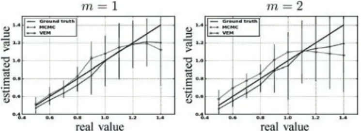
sec-tion is dedicated to studying the robustness of the spatial reg-ularization parameter estimation. For doing so, the synthetic activation maps of Fig. 2 are replaced with maps obtained as simulations of a two-class Potts model with interaction param-eter that varies from 0.5 to 1.4. When positive, this parameter favors spatial regularity across adjacent voxels, and hence smoother activation maps. Fig. 11 shows the estimated mean value and standard deviations for
over 100 simulations using both algorithms and for the two ex-perimental conditions. Three main regions can be distinguished for both experimental conditions. The Þrst one corresponds to , which approximatively matches the phase transition critical value for the two-class Potts model. For this region, Fig. 11 shows that the VEM estimate (green curve) appears to be closer to the Ground truth (black line) than the MCMC one (blue curve). Also, the proposed VEM
Fig. 10. MSE on NRL estimates split into variance (top) and squared bias (bottom) with respect to input SNR (AR(2) noise) by varying the amount of AR(2) noise autocorrelation.
Fig. 11. Reference (diagonal) and estimated mean values of with VEM MCMC for both experimental conditions ( and ). Mean values and standard deviations (vertical bars) are computed based on 100 simulations.
approach yields more accurate estimation, especially for the Þrst experimental condition having relatively high CNR. The second region corresponds to , where MCMC inference becomes more robust than VEM. The third region is identiÞed by , where both methods give less robust estimation than for the Þrst two regions. Based on these regions, we con-clude that the variational approximation (mean-Þeld) improves the estimation performance up to a given critical value. It turns out that such an approximation is more valid for low values, which usually correspond to observed values on real fMRI data.
When comparing estimates for the two conditions, the curves in Fig. 11 show that both methods generally estimate more pre-cise values for the Þrst experimental condition
having higher input CNR. For both cases, and across the three regions identiÞed hereabove, the error bars show that the VEM approach generally gives less scattered estimates (lower stan-dard deviations) than the MCMC one, which conÞrms the gain in robustness induced by the variational approximation.
Note here that estimated values in the experiment of Section IV-A-1 lie in the Þrst region for the Þrst experimental condition ( , ). For the second condition, and because low input SNR, no clear conclusion can be made since MCMC and VEM give relatively different values ( , ) and no ground truth is available since activation maps have been drawn by hand and not simulated according to the Markov model.
B. Real fMRI Datasets
This section is dedicated to the experimental validation of the proposed VEM approach in a real context. Experiments were conducted on real fMRI data collected on a single healthy adult subject who gave informed written consent. Data were collected with a 3T Siemens Trio scanner using a 3-D magnetization pre-pared rapid acquisition gradient echo (MPRAGE) sequence for the anatomical MRI and a gradient-echo echo planar imaging (GRE-EPI) sequence for the fMRI experiment. The acquisi-tion parameters for the MPRAGE sequence were set as fol-lows: time of echo: ms; time of repetition:
ms; sagittal orientation; spatial in-plane resolution: mm ; Þeld-of-view: mm and slice thickness: 1.1 mm. Regarding the EPI sequence, we used the following set-tings: the fMRI session consisted of EPI scans, each of them being acquired using ms, ms, slice thickness: 3 mm, transversal orientation, mm and spatial in-plane resolution was set to mm . Data was col-lected using a 32 channel head coil to enable parallel imaging during the EPI acquisition. Parallel SENSE imaging was used to keep a reasonable time of repetition (TR) value in the context of high spatial resolution.
The fMRI experiment design was a functional localizer par-adigm [43] that enables a quick mapping of cognitive brain functions such as reading, language comprehension and mental calculations as well as primary sensory-motor functions. It con-sists of a fast event-related design comprising sixty auditory, vi-sual and motor stimuli, deÞned in ten experimental conditions and divided in two presentation modalities (auditory and visual sentences, auditory and visual calculations, left/right aurally and visually induced motor responses, horizontal and vertical checkerboards). The average ISI is 3.75 s including all exper-imental conditions. Such a paradigm is well suited for simul-taneous detection and estimation, in contrast to slow event-re-lated and block paradigms which are considered as optimal for estimation and detection, respectively [44]. After standard pre-processing steps (slice-timing, motion corrections and normal-ization to the MNI space), the whole brain fMRI data was Þrst parcellated into functionally homogeneous parcels by resorting to the approach described in [26]. This parcellation method consisted of a hierarchical clustering (Euclidean dis-tance, Ward’s linkage) of the experimental condition effects es-timated by a GLM analysis. This GLM analysis comprised the temporal and dispersion HRF derivatives as regressors so that the clustering took some HRF variability into account. To en-force parcel connexity, the clustering process was spatially con-strained to group only adjacent positions. This parcellation was used as an input of the JDE procedure, together with the fMRI time series. We stress the fact that the latter signals were not spatially smoothed prior to the analysis as opposed to the clas-sical SPM-based fMRI processing. In what follows, we com-pare the MCMC and VEM versions of JDE with the classical GLM analysis by focusing on two contrasts of interest: 1) the
visual–auditory (VA) contrast which evokes positive and
neg-ative activity in the primary occipital and temporal cortices, respectively, and 2) the computation-sentences (CS) contrast which aims at highlighting higher cognitive brain functions.
Besides, results on HRF estimates are reported for the two JDE versions and compared to the canonical HRF, as well as maps of regularization factor estimates.
Fig. 12 shows results for the VA contrast. High positive values are bilaterally recovered in the occipital region and the overall cluster localizations are consistent for both MCMC and VEM algorithms. The only difference lies in the temporal auditory regions, especially on the right side, where VEM yields rather more negative values than MCMC. Thus VEM seems more sensitive than MCMC. The results obtained by the classical GLM (see Fig. 12 [right]) are comparable to those of JDE in the occipital region with roughly the same level of re-covered activations. However, in the central region, we observe activations in the white matter that can be interpreted as false positives and that were not exhibited using the JDE formalism. The bottom part of Fig. 12 compares the estimated values of the regularization factors between VEM and MCMC algorithms for two experimental conditions involved in the VA contrast. Since these estimates are only relevant in parcels which are activated by at least one condition, a mask was applied to hide non-activated parcels. We used the following criterion to classify a parcel as activated: (and nonactivated otherwise). These maps of estimates show that VEM yields more contrasted values between the visual and auditory conditions. Table III provides the estimated values in the highlighted parcels of interest. The auditory condition does not elicit evoked activity and yields lower values in both parcels whereas the visual condition is associated with higher values. The latter comment holds for both algorithms but VEM provides much lower values than MCMC for the non-activated condition. For the activated condition, the situation is comparable, with and . This illustrates a noteworthy difference between VEM and MCMC. Probably due to the mean Þeld and variational approximations, the hidden Þeld may not have the same behaviour (different regularization effect) between the two algorithms. Still, this discrepancy is not visible on the NRL maps.
Fig. 12(a) and (b) depicts HRF estimation results which are rather close for both methods in the two regions under consid-eration. VEM and MCMC HRF estimates are also consistent with the canonical HRF shape. Indeed, the latter has been pre-cisely calibrated on visual regions [10], [11]. These estimation results explain why JDE does not bring any gain in sensitivity compared to the classical GLM: the canonical HRF is the op-timal choice for visual areas. We can note a higher variability in the undershoot part, which can be explained, Þrst, by the fast event-related nature of the paradigm where successive evoked responses are likely to overlap in time so that it is more difÞ-cult to disentangle their ends; and second, by the lower signal strength and SNR in the tail of the response. To conclude on the VA contrast which focused on well-known sensory regions, VEM provides sensitive results consistent with the MCMC ver-sion, both with respect to detection and estimation tasks. These results were also validated by a classical GLM analysis which yielded comparable sensitivity in a region where the canonical HRF is known to be valid (see Fig. 12 [right]).
Fig. 12. Results for the VA contrast obtained by the VEM and MCMC JDE versions, compared to a GLM analysis. Top part, from left to right: NRL contrast maps for MCMC, VEM, and GLM with sagittal, coronal and axial views from top to bottom lines (neurological convention: left is left). Middle part: plots of HRF estimates for VEM and MCMC in the two parcels circled in indigo and magenta on the maps: occipital left (a) and right (b), respectively. The canonical HRF shape is depicted in dashed line. Bottom part: axial maps of estimated regularization parameters for the two conditions, auditory (aud.) and visual (vis.), involved in the VA contrast. Parcels that are not activated by any condition are hidden. For all contrast maps, the input parcellation is super-imposed in white contours.
TABLE III
ESTIMATEDREGULARIZATIONPARAMETERS OBTAINEDWITHVEM ANDMCMC JDEFOR THEEXPERIMENTALCONDITIONSINVOLVED IN THE STUDIEDCONTRASTS: VAANDCS. RESULTS AREPROVIDED FOR THETWO
HIGHLIGHTEDPARCELS FOREACHCONTRAST(SEEFig. 12 and 13)
Results related to the CS contrast are depicted in Fig. 13. As for VA, NRL contrast maps are roughly equiva-lent for VEM and MCMC in terms of cluster localizations. Still, in Fig. 13 [left-center], we observe that MCMC seems quite less speciÞc than VEM as positive contrast values are exhib-ited in the white matter for MCMC, and not for VEM (com-pare especially the middle part of the axial slices). Here, GLM results clearly show lower sensitivity compared to the JDE re-sults. For the estimates of the regularization parameters, the sit-uation is globally almost the same as for the VA contrast, with VEM yielding more contrasted maps than MCMC. However, these values are slightly lower than the ones reported for the VA contrast.
Fig. 13. Results for the CS contrast obtained by the VEM and MCMC JDE ver-sions compared to a GLM analysis. Top part, from left to right: NRL contrast maps for MCMC, VEM, and GLM, with sagittal, coronal and axial views from top to bottom lines (neurological convention: left is left). Middle part: plots of HRF estimates for VEM and MCMC in the two parcels circled in indigo and magenta on the maps: left parietal lobule (a) and left middle frontal gyrus (b), respectively. The canonical HRF shape is depicted in dashed line. Bottom part: axial maps of estimated regularization parameters for the two conditions, computation (comp.) and sentence (sent.), involved in the CS con-trast. Parcels that are not activated by any condition are hidden. For all contrast maps, the input parcellation is superimposed in white contours.
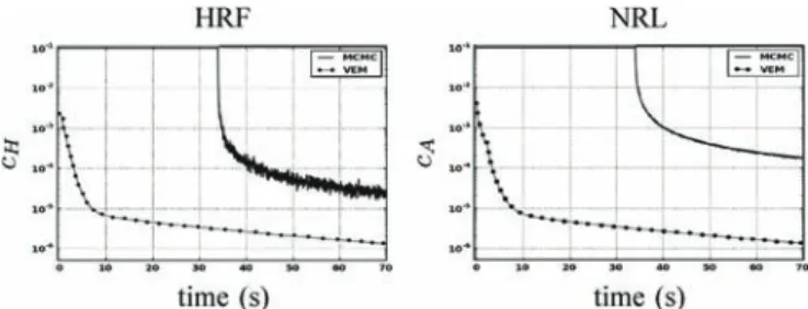
Fig. 14. Convergence curves in semi-logarithmic scale of HRF (left) and NRL (right) estimates using MCMC (blue lines) and VEM (green lines).
We Þrst focus on the left frontal cluster, located in the middle frontal gyrus which has consistently been exhibited as involved in mental calculation [45]. HRF estimates in this region are shown in Fig. 13(b) and strongly depart from the canonical ver-sion, which explains the weaker sensitivity in the GLM results as the canonical HRF model is not optimal in this region. Es-pecially, the TTP value is much more delayed with JDE (7.5 s), compared to the canonical situation (5 s). The VEM and MCMC shapes are close to each other, except at the beginning of the curves where VEM presents an initial dip. This might be in-terpreted as a higher temporal regularization introduced in the MCMC scheme. Still, the most meaningful HRF features such
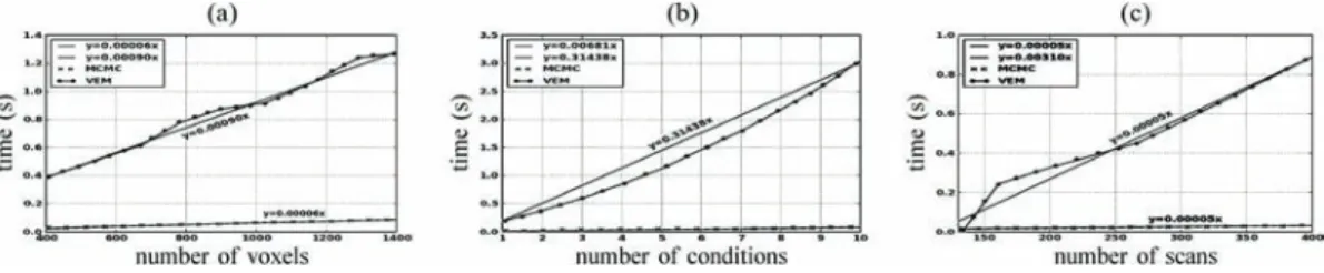
Fig. 15. Evolution of the computational time per iteration using the MCMC and VEM algorithms when varying the problem dimension according to: (a) number of voxels; (b) number of conditions; (c) number of scans.
as the TTP and the full-width at half-maximum (FWHM) are very similar.
The second region of interest for the CS contrast is located in the inferior parietal lobule and is also consistent with the compu-tation task [45]. Note that the contrast value is lower than the one estimated in the frontal region, whatever the inference scheme. Interestingly, this activation is lost by the GLM Þtting proce-dure. HRF estimates are shown in Fig. 13(a). The statement relative to the previous region holds again: they strongly differ from the canonical version, which explains the discrepancy be-tween the different detection activation results each method re-trieved. When comparing MCMC and VEM, even if the global shape and the TTP position are similar, the initial dip in the HRF estimate is still stronger with VEM and the corresponding FWHM is also smaller than for the MCMC version. As previ-ously mentioned, this suggests that MCMC may tend to over-smooth the HRF shape. Results for the regularization parame-ters, as shown in Table III [fourth column], indicate that for VEM and the Sentence condition is not as low as it is for the other parcels and the nonactivated conditions (
against ). This is explained by the fact that both Computation and the Sentence conditions yield activations in this parcel as conÞrmed by the low contrast value.
The studied contrasts represent decreasing CNR situations, with the VA contrast being the stronger and CS the weaker. From the detection point of view, the contrast maps are very similar for both JDE versions and are only dimly affected by the CNR ßuctuation. In contrast, HRF estimation results are much more sensitive to this CNR variation, with stronger discrepan-cies between the VEM and MCMC versions, especially for the HRF estimates associated with the CS parietal cluster. The latter shows the weaker contrast magnitude. Still, both versions pro-vide results in agreement on the TTP and FWHM values. In-deed, the differences mainly concern the heading and tailing parts of the HRF curves.
V. ALGORITHMICEFFICIENCY
In this section, the computational performance of the two approaches are compared on both artiÞcial and real fMRI datasets. Both algorithms were implemented in Python and fully optimized by resorting to the efÞcient array operations of the Numpy library (http://numpy.scipy.org) as well as C-ex-tensions for the computationally intensive parts (e.g., NRL sampling in MCMC or the VE-Q step for VEM). Moreover, our implementation handled distributed computing resources as the JDE analysis consists of parcel-wise independent processings which can thus be performed in parallel. This code is available
in the PyHRF package (http://www.pyhrf.org). For both the VEM and MCMC algorithms, the same stopping criterion was used. This criterion consists of simultaneously evaluating the online relative variation of each estimate. In other words, for instance for the estimated , one has to check whether . By evaluating a similar criterion for the NRLs estimates, the algorithm is Þnally stopped once and . For the MCMC algorithm, this criterion is only computed after the burn-in period, when the samples are assumed to be drawn from the target distribution. The burn-in period has been Þxed manually based on several a posteriori controls of simulated chains relative to different runs (here 1000 iterations). More sophisticated convergence monitoring techniques [46] should be used to stop the MCMC algorithm, but we chose the same criterion as for the VEM to carry out a more direct comparison. Considering the artiÞcial dataset presented in Section IV-A-1, Fig. 14 illustrates the evolution of and with respect to the computational time for both algorithms. Only about 18 s are enough to reach convergence for the VEM algorithm, while the MCMC alternative needs about 1 min to converge on the same Intel Core 4—3.20 GHz—4 Gb RAM architecture. The horizontal line in the blue curve relative to the MCMC algorithm corresponds to the burn-in period (1000 iterations). It can also be observed that the gain in computational efÞciency the VEM scheme brings is independent of the unknown variables (e.g., HRF) we look at.
To illustrate the impact of the problem dimensions on the computational cost of both methods, Fig. 15 shows the evolu-tion of the computaevolu-tional time of one iteraevolu-tion when varying the number of voxel (left), the number of experimental condi-tions (center) and the number of scans (right). The three curves show that the computational time increases almost linearly (see the blue and red curves) for both algorithms, but with different slopes. Blue curves (VEM) have steeper slopes than red ones (MCMC) in the three plots showing that the computational time of one iteration increases faster with VEM than with MCMC with respect to the problem dimensions.
As regards computational performance on the real fMRI data set presented in Section IV-B and comprising 600 parcels, the VEM also appeared faster as it took 1.5 h to perform a whole brain analysis whereas the MCMC version took 12 h. These analysis timings were obtained by a serial processing of all parcels for both approaches. When resorting to the distributed implementation, the analysis durations boiled down to 7 min for VEM and 20 min for MCMC (on a 128-core cluster). To go further, we illustrate the computational time difference
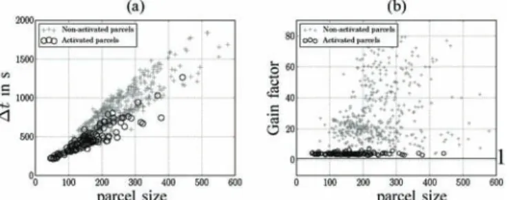
Fig. 16. Comparison of durations for MCMC and VEM analyses in terms of parcel size, each dot coding for a different parcel. (a): differential timing
. (b): gain factor of VEM compared to MCMC, horizontal line indicates a gain factor . Plus marks indicate parcels estimated as activated, i.e., and circles indicate parcels estimated as nonactivated.
between both algorithms in terms of parcel size which ranged from 50 to 580 voxels. As VEM versus MCMC efÞciency appears to be inßuenced by the level of activity within the parcel, we resorted to the same criterion as in Section IV-B to distinguish non-activated from activated parcels and tag the analysis durations accordingly in Fig. 16. Fig. 16(a) clearly shows that the differential timing between the two algorithms is higher for nonactivated parcels (blue dots) and increases with the parcel size, which conÞrms the utility of the proposed VEM approach especially in low CNR/SNR circumstances. To further investigate the gain in terms of computational time induced by VEM, Fig. 16(b) illustrates the gain factor for activated and non-activated parcels. This Þgure shows that the VEM algorithm always outperforms the MCMC alternative since in all parcels [see horizontal line in Fig. 16(b)]. Moreover, the gain factor is clearly higher for nonactivated parcels for which the input SNRs and CNRs are relatively low, and we found
.
VI. DISCUSSION ANDCONCLUSION
In this paper, we have proposed a new intra-subject method for parcel-based joint detection-estimation of brain activity from fMRI time series. The proposed method relies on a Vari-ational EM algorithm as an alternative solution to intensive stochastic sampling used in previous work [23], [25]. Com-pared to the latter formulation, the proposed VEM approach does not require priors on the model parameters for inference to be carried out. However, to achieve gain in robustness and make the proposed approach completely auto-calibrated, the adopted model can be extended by injecting additional priors on some of its parameters as detailed in Appendix E for and
estimation.
Illustrations on simulated and real datasets have been deeply conducted in order to assess the robustness of the proposed method compared to its MCMC counterpart in different exper-imental contexts. Simulations have shown that the proposed VEM algorithm retrieved more accurate activation labels and NRLs especially at low input CNR, while yielding similar performance for HRF estimation. VEM superiority in terms of NRLs and labels estimation has been conÞrmed by mean equality statistical tests over estimation errors obtained through 100 Monte Carlo runs. Conducted tests showed very low
p-values, which means that differences in terms of obtained error means were statistically signiÞcant. Simulations have also shown that our approach was more robust to any decrease of stimulus density (or equivalently to any increase of ISI value). Similar conclusions have been drawn with respect to noise level and autocorrelation structure. In addition, our VEM approach provided more robust estimation of the spatial regularization parameter and more compact activation maps that are likely to better account for functional homogeneity. These good properties of the VEM approach are obtained faster than using the MCMC implementation. Simulations have also been conducted to study the computational time variation with respect to the problem dimensions, which may signiÞcantly vary from one experimental context to another.
As a general comment, this performance of VEM compared to MCMC may be counterintuitive. The sampled chain in MCMC is supposed to converge to the true target distribution after the burn-in period. However, since non-informative priors are used in the MCMC model such as the uniform prior for Potts parameters , imprecisions in the target distribution may occur. In this case, VEM may outperform MCMC as observed in our simulations. Also, in some of the experiments, the model assumes a two-class Potts model for the activation classes while we used more realistic synthetic images instead. The images we used (e.g., the house shape) are more regular and realistic than would be a typical realization of a Potts model. Then, our results show lower MSE (variance and squared bias) for VEM when the noise model is misspeciÞed and we suspect that VEM is less sensitive to model misspeciÞcation. In a misspeciÞcation context, the variational approach may be favored by the fact that the factorization assumption acts as an extra regularizing term that smoothes out the solutions in a more appropriate manner. There exists a number of other studies in which the variational approach is compared to its MCMC counterpart and provides surprisingly accurate results [30], [38], [47], [48]. It is true that results showing the superior performance of VEM over MCMC are more seldom. For instance, the results reported in [38] show that their variational approach is highly accurate in approximating the posterior distribution. These authors show like us, smaller MSE for the variational approach versus MCMC on simulations and point out a MCMC sensitivity to initialization conditions. On a computational efÞciency point of view, most works on variational methods lead to EM-like algorithms in which one iteration consists of updating sufÞ-cient statistics (e.g., means and variances) that characterize the distribution approximating the target posterior. In our set-ting the approximaset-ting distribution is made of Gaussian parts fully speciÞed by their mean and variance. In contrast, sam-pling-based methods like MCMC are not focused on sufÞcient statistics computation, but rather simulate realizations from the full posterior. Approximating a limited number of moments is less complex than approximating a full distribution, which may also be an ingredient that explains improved VEM efÞciency and performance.
Regarding real data experiments, VEM and MCMC showed similar results with a higher speciÞcity for the former. Com-pared to the classical GLM approach, the JDE methodology yields similar results in the visual areas where the canonical
HRF is well recovered, whereas in the areas involved in the
CS contrast, the estimation of more adapted HRFs that strongly
differ from the canonical version enables higher sensitivity in the activation maps. These results further emphasize the interest of using VEM for saving a large amount of computational time. From a practical viewpoint, another advantage of the proposed algorithm lies in its simplicity to track convergence even if the latter is local: the VEM algorithm only requires a simple stop-ping criterion to achieve a local minimizer in contrast to the MCMC implementation [25]. It is also more ßexible to account for more complex situations such as those involving higher AR noise order, habituation modeling [49] or considering three in-stead of two activation classes with an additional deactivation class.
To conÞrm the impact of the proposed inference, compar-isons between the MCMC and VEM approaches should also take place at the group level. The most straightforward way would be to compare the results of random effect analyses (RFX) based on group-level Student t-test on averaged effects, the latter being computed either by a standard individual SPM analysis or by the two VEM and MCMC JDE approaches. In this direction, a preliminary study has been performed in [14] where group results based on JDE MCMC intra-subject analyses provide higher sensitivity than results based on GLM based intra-subject analyses. Ideally, the JDE framework could be extended to perform group-level analysis and yield group-level NRL maps as well as group-level HRFs. To break down the complexity, this extension could operate parcel-wisely by grouping subject-dependent data into group-level function-ally homogeneous parcels. This procedure would result in a hierarchical mixed effect model and encode mean group-level values of NRLs and HRFs so that subject-speciÞc NRL and HRF quantities would be modeled as ßuctuations around theses means.
Such group-level validations would also shed the light on the impact of the used variational approximation in VEM. In fact, no preliminary spatial smoothing is used in the JDE approach in contrast to standard fMRI analyses where this smoothing helps retrieving clearer activation clusters. In this context, the used mean Þeld approximation especially in the VE-Q step should help getting less noisy activation clusters compared to the MCMC approach. Eventually, akin to [23], the model used in our approach accounts for functional homogeneity at the parcel scale. These parcels are assumed to be an input of the proposed JDE procedure and can be a priori provided independently by any parcellation technique [26], [50]. In the present work, parcels have been extracted from functional features we obtained via a classical GLM processing assuming a canonical HRF for the entire brain. This assumption does not bias our HRF local model estimation since a large number of parcels is considered (600 parcels) with an average parcel size of 250 voxels.
However, on real dataset, results may depend on the relia-bility of the used parcellation technique. A sensitivity analysis has been performed in [51] on real data and for MCMC JDE version, that assesses the reliability of this parcellation against a computationally heavier approach which tends, by randomly sampling the seed positions of the parcels, to identify the
parcel-lation that retrieved the most signiÞcant activation maps. Still, it would be of interest to investigate the effect of the parcella-tion choice in the VEM context, and more generally to extend the present framework to incorporate an automatic online par-cellation strategy to better Þt the fMRI data while accounting for the HRF variability across regions, subjects, populations and experimental contexts. The current variational framework has the advantage to be easily augmented with parcel identiÞ-cation at the subject-level as an additional layer in the hierar-chical model. Automatically identifying parcels raises a model selection problem in the sense of getting sparse parcellation (re-duced number of parcels) which guarantees spatial variability in hemodynamic territories while enabling the reproducibility of parcel identiÞcation across fMRI datasets. More generally, a model selection approach can be easily carried out within the VEM implementation as variational approximations of standard information criteria based on penalised log-evidence can be ef-Þciently used [52].
APPENDIX
A. Derivation of the VEM Formula
We show here how to obtain the variational E-steps using the properties of the KL divergence without resorting to calculus of variation as usually done. We illustrate the approach for the derivation of the VE-H step (8). The following VE-steps can be derived similarly. Dropping the and superscripts, the VE-H step is deÞned as
DeÞnition (4) of leads to
, s.t.:
In the last equality above, we artiÞcially introduced the exponential by taking the logarithm. We then de-note by the distribution on proportional to . The normalizing constant of the latter quantity is by deÞnition independent of so that the above argmax is
where is the KL divergence between and . From the KL divergence properties, it follows that the op-timal is which provides (8) as desired.
B. VE-H Step
For the VE-H step, the expressions for and are
and with , and denoting respectively the and entries of the mean vector and covariance matrix of the current .
C. VE-A Step
The VE-A step also leads to a Gaussian pdf for
: . The parameters
are updated as and
, where a number of intermediate quantities need to be speciÞed.
First, and
where is the matrix made of columns . The th column of is then also denoted by
. Then,
and is an matrix whose element is given by
.
D. VE-Q Step
From and in Section II, it follows that the couples correspond to independent hidden Potts models with Gaussian class distributions. It fol-lows an approximation that factorizes over conditions:
where
is the posterior of in a modiÞed hidden Potts model , in which the observations ’s are replaced by their mean values and an external Þeld
is added to the prior Potts model . It follows that the deÞned Potts reads as
. Since the expression here above is intractable, and using the mean-Þeld approximation [41], is approximated by a factorized density such that if ,
, where is a particular conÞgura-tion of updated at each iteration according to a speciÞc scheme and
.
E. M Step
1) M- Step: By maximizing with respect to , (12) reads
(13)
By denoting , and after deriving with respect to and for every and
, we get and
.
2) M- Step: By maximizing with respect to , (12) reads as . Then it fol-lows the closed-form
.
For a more accurate estimation of , one may take advantage of the ßexibility of the VEM inference and inject some prior knowledge about this parameter in the model. Being positive, a suitable prior can be an exponential distribution with mean
(14) Accounting for this prior, the new expression of the current es-timate is
3) M- Step: By maximizing with respect to , (12) reads
(15)
Updating consists of making further use of a mean Þeld-like approximation [41], which leads to a function that can be opti-mized using a gradient algorithm. To avoid overestimation of this key parameter for the spatial regularization, one can intro-duce for each , some prior knowledge that pe-nalizes high values. As in (14), an exponential prior with mean can be used. The expression to optimize is then given by
After calculating the derivative with respect to , we retrieve the standard equation detailed in [41] in which
is replaced by
. It can be easily seen that, as expected, subtracting the constant helps penalizing high values.
4) M- Step: This maximization problem factorizes
over voxels so that for each , we need to compute
(16) where . Finding the maximizer with respect to leads to ( is deÞned in the VE-A step)