Pépite | Caractérisation chimique, sources et origines des aérosols inorganiques secondaires mesurés sur un site suburbain du Nord de la France

Texte intégral

(1)Thèse de Roger Roig Rodelas, Université de Lille, 2018. THESE présentée en vue d’obtenir le grade de. DOCTEUR en Sciences de la Terre et de l’Univers par. Roger ROIG RODELAS Doctorat de l’Université de Lille délivré par IMT LILLE DOUAI. Titre de la thèse:. Chemical characterization, sources and origins of secondary inorganic aerosols measured at a suburban site in Northern France. Soutenue publiquement le 29 juin 2018 devant le jury d’examen: Rapportrice Rapporteur Examinateur Examinateur Encadrante Directrice de Thèse. Magda CLAEYS Jean-Luc JAFFREZO Laurent POULAIN Olivier FAVEZ Esperanza PERDRIX Véronique RIFFAULT. Professeure émerite, University of Antwerp Directeur de Recherche, CNRS IGE Grenoble Chercheur, TROPOS Leipzig Ingénieur docteur, INERIS Maître-Assistante, IMT Lille Douai Professeure, IMT Lille Douai. Laboratoire d’accueil: Département Sciences de l’Atmosphère et Génie de l’Environnement, IMT Lille Douai Ecole Doctorale SMRE 104 (Lille, Artois, ULCO, UVHC, Centrale Lille, Chimie Lille, IMT Lille Douai). © 2018 Tous droits réservés.. lilliad.univ-lille.fr.

(2) Thèse de Roger Roig Rodelas, Université de Lille, 2018. 2 © 2018 Tous droits réservés.. lilliad.univ-lille.fr.

(3) Thèse de Roger Roig Rodelas, Université de Lille, 2018. Résumé Les particules fines troposphériques de diamètre aérodynamique inférieur à 2,5 µm (PM2.5) peuvent impacter la santé et les écosystèmes. Les aérosols inorganiques secondaires (AIS) et organiques (AO) contribuent fortement aux PM2.5. Pour comprendre leur formation et leur origine, une campagne d’1 an (août 2015 - juillet 2016) de mesures horaires de gaz précurseurs inorganiques et d’ions hydrosolubles particulaires a été menée sur un site suburbain du nord de la France avec un MARGA 1S, complétées par les concentrations massiques en PM2.5, carbone suie, oxydes d’azote et éléments traces. Des niveaux élevés de nitrate d’ammonium (NA) ont été observés la nuit au printemps et de sulfate d’ammonium la journée en été. L’étude de la contribution des sources par le modèle PMF (Positive Matrix Factorization) a permis d’identifier 8 facteurs sources: 3 régionaux (riche en sulfates, riche en nitrates et marin) pour 73 à 78%, et 5 locaux (trafic, combustion de biomasse, fond industriel métallurgique, industrie locale et poussières minérales) (22-27%). De plus, un HR-ToF-AMS (spectromètre de masse à aérosols) et un SMPS (granulomètre) ont été utilisés lors d’une campagne intensive en hiver, afin de mieux documenter l’AO et la formation de nouvelles particules, respectivement. L’application du PMF aux spectres de masses d’AO a permis d’identifier 5 facteurs liés au trafic (15%), à la cuisson (11%), à la combustion de biomasse (25%), et à une oxydation plus ou moins forte de la matière organique (33% et 16%). Plusieurs événements nocturnes de formation de nouvelles particules impliquant les AIS, notamment du NA, ont été observés.. Mots clés: particules fines, aérosol inorganique secondaire, aérosol organique, gaz précurseur, nitrate d’ammonium, spectrométrie de masse à aérosols, identification de sources, Positive Matrix Factorization. 3 © 2018 Tous droits réservés.. lilliad.univ-lille.fr.

(4) Thèse de Roger Roig Rodelas, Université de Lille, 2018. Abstract Tropospheric fine particles with aerodynamic diameters less than 2.5 µm (PM2.5) may impact health, climate and ecosystems. Secondary inorganic (SIA) and organic aerosols (OA) contribute largely to PM2.5. To understand their formation and origin, a 1-year campaign (August 2015 to July 2016) of inorganic precursor gases and PM2.5 water-soluble ions was performed at an hourly resolution at a suburban site in northern France using a MARGA 1S, complemented by mass concentrations of PM2.5, Black Carbon, nitrogen oxides and trace elements. The highest levels of ammonium nitrate (AN) and sulfate were observed at night in spring and during daytime in summer, respectively. A source apportionment study performed by positive matrix factorization (PMF) determined 8 source factors, 3 having a regional origin (sulfate-rich, nitrate-rich, marine) contributing to PM2.5 mass for 73-78%; and 5 a local one (road traffic, biomass combustion, metal industry background, local industry and dust) (2227%). In addition, a HR-ToF-AMS (aerosol mass spectrometer) and a SMPS (particle sizer) were deployed during an intensive winter campaign, to gain further insight on OA composition and new particle formation, respectively. The application of PMF to the AMS OA mass spectra allowed identifying 5 source factors: hydrocarbon-like (15%), cooking-like (11%), oxidized biomass burning (25%), less- and more-oxidized oxygenated factors (16% and 33%, respectively). Combining the SMPS size distribution with the chemical speciation of the aerosols and precursor gases allowed the identification of nocturnal new particle formation (NPF) events associated to the formation of SIA, in particular AN. Keywords: fine particles, secondary inorganic aerosols, organic aerosols, precursor gases, ammonium nitrate, aerosol mass spectrometry, sources apportionment, Positive Matrix Factorization. 4 © 2018 Tous droits réservés.. lilliad.univ-lille.fr.

(5) Thèse de Roger Roig Rodelas, Université de Lille, 2018. Table of contents. List of Figures .......................................................................................................................... 10 List of tables ............................................................................................................................. 14 List of Abbreviations ................................................................................................................ 15 GENERAL INTRODUCTION ................................................................................................ 21 CHAPTER 1. Atmospheric Context ........................................................................................ 29 1.1. General introduction to atmospheric aerosols ........................................................... 29. 1.1.1 Definition of atmospheric particulate matter (PM) ................................................. 29 1.1.2 Size of aerosols ........................................................................................................ 29 1.1.3 Sources ..................................................................................................................... 31 1.1.4 Aerosol life cycle ..................................................................................................... 39 1.1.5 Chemical composition of aerosols ........................................................................... 41 1.1.6 Effects ...................................................................................................................... 44 1.1.7 Legal framework ...................................................................................................... 47 1.2. Secondary inorganic aerosols (SIA) .......................................................................... 48. 1.2.1 Sulfur species ........................................................................................................... 48 1.2.2 Nitrogen species....................................................................................................... 52 1.2.3 Neutralization reactions for SIA formation ............................................................. 55 1.2.4 Ammonium nitrate formation .................................................................................. 56 1.3 Techniques for the measurement of aerosols and gaseous precursors in the ambient air…… .................................................................................................................................. 60 1.3.1 Offline measurements .............................................................................................. 60 1.3.2 Online measurements............................................................................................... 62 1.4. Source apportionment ................................................................................................ 62. 1.4.1 Source receptor models............................................................................................ 62 1.4.2 Positive matrix factorization (PMF) ........................................................................ 64 1.4.3 PM2.5 source apportionment with PMF in North-Western Europe .......................... 65 1.5. Work motivation ........................................................................................................ 66. 1.5.1 Pollution in Northern France ................................................................................... 66 1.5.2 Previous studies in the region of Northern France .................................................. 69 1.5.3 Issues in air quality modelling ................................................................................. 71 1.6. Objectives and scientific strategy .............................................................................. 75 5. © 2018 Tous droits réservés.. lilliad.univ-lille.fr.

(6) Thèse de Roger Roig Rodelas, Université de Lille, 2018. 1.7. References ................................................................................................................. 78. CHAPTER 2. Materials and methods ...................................................................................... 89 2.1. Location of the campaign and summary of the instrumentation used ....................... 89. 2.1.1 Site description ........................................................................................................ 89 2.1.2 Air quality in Douai ................................................................................................. 90 2.1.3 Instrumentation ........................................................................................................ 93 2.2. MARGA .................................................................................................................... 96. 2.2.1 Description ............................................................................................................... 96 2.2.2 Literature review .................................................................................................... 101 2.2.3 Data validation ....................................................................................................... 112 2.2.4 Detection limit calculations ................................................................................... 113 2.3. Aethalometer ........................................................................................................... 114. 2.4. Partisol 2300 – filter sampling and ICP-MS analysis of trace and major elements 116. 2.5. BAM-1020 ............................................................................................................... 117. 2.6. Gas monitors ............................................................................................................ 118. 2.6.1 NOx ........................................................................................................................ 118 2.6.2 SO2 ......................................................................................................................... 118 2.7. HR-ToF-AMS .......................................................................................................... 119. 2.7.1 Description and operating principle....................................................................... 119 2.7.2 Data collection ....................................................................................................... 120 2.7.3 Data analysis .......................................................................................................... 121 2.7.4 Calibrations of the AMS ........................................................................................ 124 2.8. Scanning Mobility Particle Sizer (SMPS) ............................................................... 127. 2.9. Calculation of uncertainties ..................................................................................... 129. 2.9.1 MARGA ................................................................................................................ 129 2.9.2 Filter sampling and ICP-MS analysis of trace and major elements....................... 130 2.10 Ratios for the analysis of the aerosol acidity and the oxidation of nitrogen and sulfur ................................................................................................................................. 132 2.11 Source apportionment .............................................................................................. 134 2.11.1. Application of PMF to hourly to daily-resolved data of inorganic compounds..... .......................................................................................................................... 134. 2.11.2. Application of PMF to mass spectrometry data of organic compounds .......... 136. 2.12 Geographical determination of sources ................................................................... 137 2.12.1. Local sources .................................................................................................... 137 6. © 2018 Tous droits réservés.. lilliad.univ-lille.fr.

(7) Thèse de Roger Roig Rodelas, Université de Lille, 2018. 2.12.2. Distant sources ................................................................................................. 138. 2.13 Thermodynamic partitioning analysis: ISORROPIA II .......................................... 140 2.14 References ............................................................................................................... 142 CHAPTER 3. Characterization and variability of inorganic aerosols and their gaseous precursors at a suburban site in northern France over one year (2015-2016) (ARTICLE 1) 149 1.. Introduction ..................................................................................................................... 152. 2.. Materials and methods .................................................................................................... 154 2.1.. Campaign description .............................................................................................. 154. 2.2.. Instrumentation ........................................................................................................ 155. 2.3.. Ratios (NR and GR) ................................................................................................ 156. 2.4.. Weather and trajectory models ................................................................................ 156. 2.4.1. Non-parametric wind regression............................................................................ 156 2.4.2. Back-trajectory calculations .................................................................................. 157 2.4.3. Potential source contribution function ................................................................... 157 2.5. 3.. Thermodynamic module .......................................................................................... 158. Results ............................................................................................................................. 158 3.1.. PM2.5 chemical composition and correlations between species .............................. 158. 3.2.. Seasonal daily variability of precursor gases and inorganic aerosol species .......... 162. 3.2.1. Precursor gases ...................................................................................................... 162 3.2.2. Aerosols ................................................................................................................. 167 3.3.. Study of ratios and SIA partitioning ........................................................................ 172. 3.3.1. Ammonium neutralization ratio (NR) and gas ratio (GR) ..................................... 172 3.3.2. Hourly gas-aerosol partitioning of SIA ................................................................. 175 3.4.. Source identification ................................................................................................ 177. 3.4.1. Local sources ......................................................................................................... 177 3.4.2. Distant sources ....................................................................................................... 179 3.5.. Characteristics of high daily PM2.5 concentrations.................................................. 181. 4.. Conclusions ..................................................................................................................... 184. 5.. Data availability .............................................................................................................. 185. 6.. Acknowledgements ......................................................................................................... 185. 7.. References ....................................................................................................................... 185. CHAPTER 4. Real-time assessment of wintertime organic aerosol characteristics and sources at a suburban site in northern France ..................................................................................... 193 1.. Introduction ..................................................................................................................... 196 7. © 2018 Tous droits réservés.. lilliad.univ-lille.fr.

(8) Thèse de Roger Roig Rodelas, Université de Lille, 2018. 2.. Materials and methods .................................................................................................... 198 2.1. Measurement site ......................................................................................................... 198 2.2. Instrumentation ............................................................................................................ 198 2.3. Source apportionment of OA ....................................................................................... 200 2.4. Geographical determination of sources ....................................................................... 200 2.5. Ventilation coefficient ................................................................................................. 202. 3.. Results and discussion .................................................................................................... 202 3.1. Overview of NR-PM1 .................................................................................................. 202 3.2. OA characteristics........................................................................................................ 204 3.3. Source apportionment of OA ....................................................................................... 206 3.3.1. HOA ...................................................................................................................... 207 3.3.2. COA ...................................................................................................................... 209 3.3.3. oBBOA ................................................................................................................. 211 3.3.4. LO-OOA and MO-OOA ....................................................................................... 212 3.4. Impact of meteorological parameters and long range transport on NR-PM1 characteristics ..................................................................................................................... 213. 4.. Conclusions ..................................................................................................................... 216. 5.. Acknowledgements ......................................................................................................... 217. 6.. References ....................................................................................................................... 218. CHAPTER 5. Effect of high temporal resolution and database composition on source apportionment of PM2.5 using positive matrix factorization .................................................. 227 1. Introduction ........................................................................................................................ 230 2. Materials and methods ....................................................................................................... 232 2.1. Site description ............................................................................................................ 232 2.2. Instrumentation ............................................................................................................ 233 2.3. Source apportionment .................................................................................................. 234 2.4. Geographical determination of sources ....................................................................... 236 2.4.1. Non-parametric wind regression (NWR) .............................................................. 236 2.4.2. Potential source contribution function (PSCF) ..................................................... 236 3. Results and discussion ........................................................................................................ 238 3.1. Dataset presentation ..................................................................................................... 238 3.2. Hourly PMF results ..................................................................................................... 239 3.3. Daily PMF results ........................................................................................................ 247 3.4. Geographical determination of source factors ............................................................. 254 8 © 2018 Tous droits réservés.. lilliad.univ-lille.fr.

(9) Thèse de Roger Roig Rodelas, Université de Lille, 2018. 3.5. Comparison with other SA studies .............................................................................. 258 4. Conclusions ........................................................................................................................ 260 5. Acknowledgements ............................................................................................................ 262 6. References .......................................................................................................................... 262 CONCLUSIONS AND PERSPECTIVES ............................................................................. 271 ANNEX 0: Scientific Valorization ........................................................................................ 281 ANNEX 1: Detection limits for major and trace elements .................................................... 282 ANNEX 2: Supplementary material for Article 1 .................................................................. 284 ANNEX 3: Supplementary material for Article 2 .................................................................. 318 ANNEX 4: Supplementary material for Article 3 .................................................................. 331. 9 © 2018 Tous droits réservés.. lilliad.univ-lille.fr.

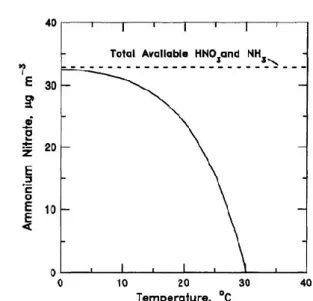
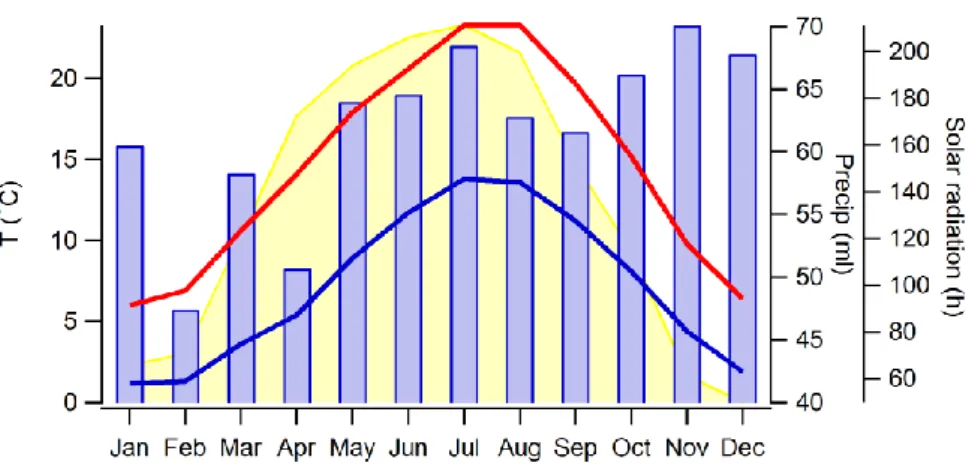
(10) Thèse de Roger Roig Rodelas, Université de Lille, 2018. List of Figures Figure 1.1 Representation of aerosol size distribution and main processes of the aerosol life cycle (Buseck and Adachi, 2008) ............................................................................................. 31 Figure 1.2 (a) Emission shares of NOx for EEA member countries for 2011 and (b) atmospheric emissions of NOx (in Kt per year) in the metropolitan France; *2016= Estimation (CITEPA, 2017) ....................................................................................................................... 35 Figure 1.3 (a) Emission shares of SO2 for EEA member countries for 2011 and (b) atmospheric emissions of SO2 (in Kt per year) in the metropolitan France; *2016= Estimation (CITEPA, 2017) ....................................................................................................................... 37 Figure 1.4 (a) Emission shares of NH3 for EEA member countries for 2011 and (b) atmospheric emissions of NH3 (in Kt per year) in the metropolitan France; *2016= Estimation (CITEPA, 2017) ....................................................................................................................... 38 Figure 1.5 Representation of the nucleation process from H2SO4, NH3, organics and other ions (Pierce, 2011) ........................................................................................................................... 40 Figure 1.6 Average size distribution of main aerosol ions (Seinfeld and Pandis, 2006) ......... 42 Figure 1.7 PM2.5 relative average composition at different European sites (Putaud et al., 2010) .................................................................................................................................................. 44 Figure 1.8 Deposition potential of PM depending on the size (Kim et al., 2015) ................... 45 Figure 1.9 Predicted average gain in life expectancy (in months) for 30-year old aged people in 25 European cities for a decrease in the annual average PM2.5 level to the WHO recommendation of 10 µg m-3 (Aphekom report) .................................................................... 45 Figure 1.10 Scattering of a radiation beam by (A) reflection, (B) refraction, (C) refraction and internal reflection and (D) diffraction (Jacob, 1999) ............................................................... 46 Figure 1.11 Comparison of aqueous-phase main oxidation pathways at 298 K (Seinfeld and Pandis, 2006) ............................................................................................................................ 52 Figure 1.12 NH4NO3 concentration dependence on temperature for a system with 7 and 26.5 µg m-3 of NH3 and HNO3, respectively, and RH 30% (from Seinfeld and Pandis, 2006) ....... 56 Figure 1.13 Deliquescence and efflorescence curves for some hygroscopic salts in relation to RH at 20 °C (Hidy, 1984)......................................................................................................... 59 Figure 1.14 Schematic of a denuder-filter pack (Limón-Sánchez et al., 2002) ....................... 61 Figure 1.15 Synthesis of the different receptor models used for estimating pollution source contributions (from Viana et al., 2008) .................................................................................... 63 Figure 1.16 Maps of France (left, in red the Hauts-de-France) and of the Hauts-de-France region (right). ........................................................................................................................... 67 Figure 1.17 Monthly averaged meteorological trends from 1981 to 2010 (blue and red curves: minimum and maximum temperatures; blue bars: cumulative precipitations; shaded yellow area: solar radiation) ................................................................................................................. 68 Figure 1.18 PM2.5 seasonal averages (Wi: winter, Sp: spring; Su: Summer; Au: Autumn) measured in the station of Douai Theuriet between 2010 and 2016 ........................................ 68 Figure 1.19 Measured and modelled monthly concentrations for NO3- (a), NH4+ (b), SO42- (c), HNO3 (d) and NH3 (e) (Schaap et al., 2011) ............................................................................ 73 Figure 1.20 Measured and modelled daily concentrations for NO3- (a), SO42- (b) and NH4+ (c) (Schaap et al., 2011) ................................................................................................................. 74 10 © 2018 Tous droits réservés.. lilliad.univ-lille.fr.

(11) Thèse de Roger Roig Rodelas, Université de Lille, 2018. Figure 1.21 Measured and modelled hourly concentrations for NO3- (a), NH4+ (b), SO42- (c), HNO3 (d) and NH3 (e) (Schaap et al., 2011) ............................................................................ 75 Figure 2.1 Maps of France (left) and “Hauts-de-France” (right) ............................................. 90 Figure 2.2 Map of Douai showing the urban area (shaded grey area), main roads (orange lines), rivers (blue lines), railroad track (black line), industrial activities (blue symbols) and sampling site (red symbol). ...................................................................................................... 91 Figure 2.3 View of the Portakabin where the permanent instrumentation was located (left) and MARGA 1S setup (right) ......................................................................................................... 95 Figure 2.4 OMEGA trailer (left) where the HR-ToF-AMS (right) was installed .................... 95 Figure 2.5 MARGA front view (left) and flow diagram (right) ............................................... 96 Figure 2.6 (a) Sample box front view; (b) WRD and (c) SJAC schematics ............................ 98 Figure 2.7 (a) Detector box front view; (b) syringe pumps; (c) sampling valves; (d) ion chromatographs ........................................................................................................................ 99 Figure 2.8 Example of calculated retention times for the anions ........................................... 100 Figure 2.9 Air flow control box ............................................................................................. 101 Figure 2.10 HR-ToF-AMS diagram (DeCarlo et al., 2006) ................................................... 120 Figure 2.11 Data collection configuration for the campaign carried out in Douai ................ 121 Figure 2.12 Flow calibration curve for the campaign carried out in Douai ........................... 125 Figure 2.13 Velocity of the particle relative to the aerodynamic diameter ............................ 127 Figure 2.14 Schematics of the DMA (left) and the CPC (right) ............................................ 128 Figure 2.15 Fishbone diagram of the main sources of uncertainty in the analysis of aerosols and gases by the MARGA ...................................................................................................... 129 Figure 2.16 Fishbone diagram of sources of uncertainty for metals ...................................... 131 Figure 2.17 Scheme of the deconvolution of the organic matrix X into two different factors and a residual matrix (Zhang et al., 2011).............................................................................. 136 Figure P1.1 Maps of France (left) and Douai (right) with the sampling site (yellow cross), the main roads (red lines), railroad (black line), city center (grey area), non-ferrous metal industry (brown area), slaughterhouse (green cross) and waste water treatment plant (WWTP, blue cross). ..................................................................................................................................... 154 Figure P1.2 PM2.5 average monthly (a) mass concentration and (b) relative contribution for the major chemical species, ND: not determined, BC: Black carbon. ................................... 161 Figure P1.3 Average daily profiles of (a) NO, (b) NO2, (c) O3, (d) HONO, (e) NH3, (f) SO2 for each season (winter: blue; spring: green, summer: red, autumn: brown). * O3 was obtained from the Atmo-HdF station in Douai Theuriet....................................................................... 163 Figure P1.4 HONO vs. NOx concentrations for (a) all daytime-averaged points and (b) data averaged over rush hours (6:00-10:00 am). ........................................................................... 164 Figure P1.5 Daily profiles of (a) PM2.5, (b) NO3-, (c) NH4+, (d) SO42-, (e) C2O42-, (f) Na+, (g) Cl-, (h) Mg2+, (i) Ca2+, (j) K+, and (k) BC for each season (winter: blue; spring: green, summer: red, autumn: brown). ............................................................................................... 169 Figure P1.6 Neutralization ratio (NR) daily profiles for each season, with the corresponding seasonal averages. .................................................................................................................. 173 Figure P1.7 (a) Observed vs. predicted NH4+ colored by Na+ concentration; and (b) NWR annual plot for the neutralization ratio (NR). ......................................................................... 174 11 © 2018 Tous droits réservés.. lilliad.univ-lille.fr.

(12) Thèse de Roger Roig Rodelas, Université de Lille, 2018. Figure P1.8 Comparison between ISORROPIA II predicted values and MARGA measurements for (a) NH3, (b) HNO3, (c) NH4+, and (d) NO3-.............................................. 176 Figure P1.9 NWR plots for the main precursor gases and particulate ions (concentrations in µg m-3) over the whole field campaign. The radial and tangential axes represent the wind direction and speed in km h-1, respectively. ........................................................................... 178 Figure P1.10 PSCF analysis for the three main particulate ions. The selected threshold is set at the 75th percentile. All used back-trajectories were weighted using a sigmoidal function. ... 180 Figure P1.11 (a) Number of hours when hourly PM2.5 is above 25 µg m-3. (b) Average chemical composition for PM2.5 hourly mass concentrations above 25 µg m-3 and (c) below 25 µg m-3 ................................................................................................................................ 182 Figure P2.1 Time series of NR-PM1, elemental ratios (OM:OC, H:C and O:C) and of the main meteorological parameters (T: temperature, RH: relative humidity, P: atmospheric pressure, WD: wind direction and WS: wind speed) ............................................................. 203 Figure P2.2 Median daily profiles for OM:OC, O:C, H:C and N:C ...................................... 206 Figure P2.3 Van Krevelen diagram for all the data colored by time, with identified PMF factors (HOA: Hydrogen-like OA, COA: cooking-like OA; oBBOA: oxidized biomass burning OA, MO-OOA: more oxidized – oxygenated OA, LO-OOA: less oxidized – oxygenated OA). .................................................................................................................... 206 Figure P2.4 (a) Factor profiles with fragments colored by chemical families, and (b) time series of the concentrations and mass fractions of the PMF factors (HOA: Hydrogen-like OA, COA: cooking-like OA; oBBOA: oxidized biomass burning OA, MO-OOA: more oxidized – oxygenated OA, LO-OOA: less oxidized – oxygenated OA). ............................................... 208 Figure P2.5 Daily profiles of PMF factors by (a) concentration and (b) contribution to OA (HOA: Hydrogen-like OA, COA: cooking-like OA; oBBOA: oxidized biomass burning OA, MO-OOA: more oxidized – oxygenated OA, LO-OOA: less oxidized – oxygenated OA). . 209 Figure P2.6 NWR plots for AMS PMF factors, colored by mass concentration (radius: wind speed in km h-1). HOA: Hydrogen-like OA, COA: cooking-like OA; oBBOA: oxidized biomass burning OA, MO-OOA: more oxidized – oxygenated OA, LO-OOA: less oxidized – oxygenated OA. ...................................................................................................................... 210 Figure P2.7 Averaged mass concentrations and relative contributions of PMF factors as a function of RH bins (the width of the bins, represented by the horizontal bars, was chosen to increase the representativeness of each interval, with n ≥ 40). HOA: Hydrogen-like OA, COA: cooking-like OA; oBBOA: oxidized biomass burning OA, MO-OOA: more oxidized – oxygenated OA, LO-OOA: less oxidized – oxygenated OA. ................................................ 212 Figure P2.8 Average chemical composition of NR-PM1 for (a) period I and (b) period II. The OA fraction (highlighted in light green) is subdivided into its PMF factors. ........................ 215 Figure P3.1 (Left) PMFh factor profiles with concentrations (shaded grey bars) in µg m-3 and contributions (red dots) in % for every species; (Right) Time series of PMFh factors together with the main tracer of each source. ....................................................................................... 241 Figure P3.2 (Left) annual and (right) seasonal average contributions (in %) of PMFh source factors to PM2.5 (modeled concentrations) ............................................................................. 242 Figure P3.3 Daytime and nighttime averaged contributions (in %) of PMFh source factors to PM2.5 (modeled concentrations) ............................................................................................. 244 12 © 2018 Tous droits réservés.. lilliad.univ-lille.fr.

(13) Thèse de Roger Roig Rodelas, Université de Lille, 2018. Figure P3.4 Daily variations of PMFh factor concentrations (in µg m-3) for every season and for the whole year. .................................................................................................................. 245 Figure P3.5 Daily variations of (a) sulfate-rich, (b) nitrate-rich and (c) road traffic concentrations (in µg m-3) together with the main trace gases for each source ..................... 246 Figure P3.6 PMFd source profiles with the concentrations (shaded grey bars) in µg m-3 and contributions (red dots) in % for every species. MIB: Metal Industry Background. ............. 248 Figure P3.7 Time series of PMFd factors together with the main tracer for each source (concentrations in µg m-3). MIB: Metal Industry Background. ............................................. 249 Figure P3. 8 Annual (left) and seasonal (right) average contributions (in %) of PMFd source factors to PM2.5 (modeled concentrations). MIB: Metal Industry Background. .................... 251 Figure P3.9 Comparison of the species concentrations (shaded bars, in µg m-3) and contributions (filled circles, in %) for the common factors between PMFd (in blue) and PMFh (in red) approaches (only common species are shown). ........................................................ 254 Figure P3.10 Annual NWR plots of PMFh and PMFd factor concentrations (in µg m-3) per wind direction. The radial axis represents the wind speed in km h-1...................................... 255 Figure P3.11 Annual PSCF probability maps for PMFh factors identified as regional. The selected threshold is set at the 75th percentile. All used backtrajectories were weighted using a sigmoidal function. ................................................................................................................. 256 Figure P3.12 Comparison of the relative contributions of sources to PM2.5 (in %) between various western European sites where the site typology and average PM mass concentration (in µg m-3) are indicated below each bar. ............................................................................... 259. 13 © 2018 Tous droits réservés.. lilliad.univ-lille.fr.

(14) Thèse de Roger Roig Rodelas, Université de Lille, 2018. List of tables Table 1.1 Global emission estimates for major aerosol classes ............................................... 32 Table 1.2 Inorganic tracers associated with industrial activities and traffic ............................ 36 Table 1.3 Settling velocities of aerosol particles at 1 atm (adapted from Hinds, 1999) .......... 41 Table 1.4 Main characteristics of coarse and fine particles ..................................................... 42 Table 1.5 Dependence of the dissociation coefficient on temperature (T, in K) ..................... 57 Table 1.6 Thermodynamic cases for ammonium nitrate dissociation ...................................... 57 Table 1.7 DRH and concentration for saturated solutions at 25°C (Hidy, 1984) .................... 59 Table 1.8 Equilibrium state of ammonium nitrate and its precursor gases with relation to temperature and RH ................................................................................................................. 60 Table 1.9 Distribution of estimated regional emissions in the Nord-Pas-de-Calais region for 2008 (emission inventory from Atmo Nord- Pas-de-Calais) ................................................... 69 Table 2.1 Summary of main industrial activities in Douai and its surroundings by wind sector .................................................................................................................................................. 92 Table 2.2 Summary of the used instrumentation in the field campaign ................................... 94 Table 2.3 Experimental detection limits of the MARGA ...................................................... 103 Table 2.4 Characteristics and results of the comparisons between MARGA and filter-based measurements published in recent studies ............................................................................. 107 Table 2.5 Comparison results of the MARGA SO2 against two SO2 monitors ..................... 109 Table 2.6 Characteristics and results of the comparison between the MARGA and the AMS ................................................................................................................................................ 109 Table 2.7 Summary of the performance of the MARGA based on the comparison between two MARGA units performed by Rumsey et al. (2014) ........................................................ 111 Table 2.8 This study and manufacturer DLs for every species analyzed by the MARGA (in µg m-3) ......................................................................................................................................... 114 Table 2.9 Fragments (m/z) used for the determination of major chemical species in low resolution mode (from Canagaratna et al., 2007) ................................................................... 123 Table 2.10 Summary of the different calibrations and their frequency during the campaign in Douai ...................................................................................................................................... 124 Table P1.1 Statistical summary (mean ± one standard deviation) of meteorological parameters for each season ....................................................................................................................... 159 Table P1.2 Statistical summary of all measured parameters at the site of Douai for each season: average, standard deviation (SD) and percentiles (Pi) are concentrations in µg m-3; nv>D: percentage of valid data, i.e. above the detection limit (DL) for each compound ........ 160 Table P1.3 Summary of ambient HONO/NOx ratios reported in this work and other studies ................................................................................................................................................ 166 Table P1.4 Summary of PM2.5 chemical composition for each high concentration episode (concentrations in µg m-3) ...................................................................................................... 183 Table P3.1 Main statistics for the input data as used in PMFh (7862 points) and PMFd (298 points) (concentrations are in µg m-3 except for elements analyzed by ICP-MS (from Ca to Zn) which are in ng m-3). ........................................................................................................ 240. 14 © 2018 Tous droits réservés.. lilliad.univ-lille.fr.

(15) Thèse de Roger Roig Rodelas, Université de Lille, 2018. List of Abbreviations AE: AIM-IC: AMS: BAM: BBOA: BC: BVOC: CCN: CDCE: CE: CMB: COA: CPC: CTM: C-ToF-AMS: CV: DL: DMA: DMPS: DMS: DRH: EC: EEA: EMEP: EPA: ERH: FCB: GAC: GPIC: GR: GV: HEPA: HOA: HPLC: HR: HR-ToF-AMS: HYSPLIT: IB: IC: ICP-MS: IE: LO-OOA:. Aethalometer Ambient Ion Monitor – Ion chromatography Aerosol Mass Spectrometer Beta Attenuation Monitor Biomass burning-like aerosol Black carbon Biogenic volatile organic compound Cloud condensation nuclei Composition-dependent collection efficiency Collection efficiency Chemical mass balance Cooking-like aerosol Condensation Particle Counter Chemistry Transport Model Compact Time-of-Flight Aerosol Mass Spectrometer Coefficient of variation Detection limit Differential Mobility Analyzer Differential Mobility Particle Sizer Dimethyl sulfide Deliquescence relative humidity Elemental carbon European Economic Area European Monitoring and Evaluation Program United States Environmental Protection Agency Efflorescence relative humidity Flow control box Gas and Aerosol Collector Gas Particle Ion Chromatography Gas ratio Guideline value High Efficiency Particle Arrestance Hydrocarbon-like organic aerosol High performance liquid chromatography High resolution High-Resolution Time-of-Flight Aerosol Mass Spectrometer HYbrid Single-Particle Lagrangian Integrated Trajectory Ionic balance Ion chromatography Inductively Coupled Plasma – Mass Spectrometry Ionization efficiency Less oxidized - oxygenated organic aerosol 15. © 2018 Tous droits réservés.. lilliad.univ-lille.fr.

(16) Thèse de Roger Roig Rodelas, Université de Lille, 2018. LOTOS-EUROS: LRT: LV: MARGA: MCP: MDRH: ME: MEL: MFC: MO-OOA: MS: MU: NOR: NPF: NR: NR-PM1: NWR: OA: oBBOA: OM: OOA: PAH: PBL: PCA: PE: PFA: PIKA: PILS: PM: PMF: PNSD: POA: POP: PSCF: PTFE: PToF: QC: RIE: RH: RM: SCOA: SCR: SIA: SJAC:. Long Term Ozone Simulation – European Operational Smog Long-range transport Limit value Monitor for Gases and AeRosols in ambient Air Multichannel Plate Mutual deliquescence relative humidityx Multilinear Engine European Metropolis of Lille Mass Flow Controller More oxidized – oxygenated organic aerosol Mass Spectrometry Marga Unit Nitrogen oxidation ratio New particle formation event Neutralization ratio Non-refractory fine particles Non-parametric wind regression Organic aerosol Oxidized biomass burning-like aerosol Organic matter Oxygenated organic aerosol Polycyclic aromatic hydrocarbons Planetary Boundary Layer Principal Component Analysis Polyethylene Perfluoroalkoxy Peak Integration by Key Analysis Particle-Into-Liquid-Sampler Particulate matter Positive matrix factorization Particle number size distribution Primary organic aerosol Persistent organic pollutant Potential source contribution function Polytetrafluoroethylene Particle time of flight Quality control Relative ionization efficiency Relative humidity Receptor model Sulfur-containing organic aerosol Selective catalytic reduction system Secondary inorganic aerosols Steam Jet Aerosol Collector 16. © 2018 Tous droits réservés.. lilliad.univ-lille.fr.

(17) Thèse de Roger Roig Rodelas, Université de Lille, 2018. SMPS: SNR: SOA: SOR: SQUIRREL: T: TEOM-FDMS: UMR: UTC: VK: VOC: WHO: WRD: WSII:. Scanning Mobility Particle Sizer Signal-to-noise ratio Secondary inorganic aerosols Sulfur oxidation ratio SeQUential Igor data RetRIEvaL Temperature Tapered Element Oscillation Monitor – Filter Dynamics Measurement System Unit mass resolution Universal Time Coordinated Van Krevelen Volatile organic compound World Health Organization Wet Rotating Denuder Water soluble inorganic ions. 17 © 2018 Tous droits réservés.. lilliad.univ-lille.fr.


(19) Thèse de Roger Roig Rodelas, Université de Lille, 2018. GENERAL INTRODUCTION. 19 © 2018 Tous droits réservés.. lilliad.univ-lille.fr.


(21) Thèse de Roger Roig Rodelas, Université de Lille, 2018. GENERAL INTRODUCTION The interest in atmospheric aerosols or particulate matter (PM) has grown large in the last decades due to their numerous effects towards the climate (Hallquist et al., 2009), environment (EEA, 2017) and most notably, human health (Kelly and Fussell, 2012). Only in the year 2016, ambient air pollution was responsible for 4.2 million deaths worldwide, mostly due to the inhalation of particulate matter (WHO, 2018). In Europe, the premature mortality associated to ambient air pollution is also alarmingly high, with estimations for the year 2012 ranging from 190,000 to 289,000 for low- to middle-income and high-income countries, respectively (WHO, 2016) . In France alone, a comprehensive study reported an annual average of 48,000 premature deaths related to PM2.5 exposure (Santé publique France, 2016). Particularly the region of northern France is frequently affected by high ambient levels of PM2.5. These recurring particulate pollution events are partly attributed to the presence of industrialized, agricultural or highly populated areas nearby despite of the flat topography which favors the dispersion of pollutants. While SIA is a great contributor to PM2.5 in northwestern Europe (Putaud et al., 2010), it has previously been shown that in the north of France there is a particularly high contribution of biomass burning emissions during wintertime (Joaquin, 2015). In order to reduce the PM2.5 levels, it is necessary to apply effective pollution reduction strategies. A good knowledge on the sources of PM and its composition is therefore necessary both at the local and regional scales. A common and effective approach is the identification of PM sources by the use of statistical receptor models applied to a database of pollutants collected at a given location, also known as source apportionment. However, up to date most source apportionment studies have been carried out with low time resolution databases, which do not provide information about the (trans)formation processes of the aerosols or the change of pollution sources at a high time resolution, and are rather a reflection of the long-term equilibrium. This hampers the understanding of source patterns, which might be essential in the implementation of mitigation policies (Peng et al., 2016). In this context, the main goal of this work is to improve the scientific knowledge on SIA and their precursor gases, as well as on their main drivers and their interaction with other particulate constituents. For this purpose, a MARGA 1S (Monitor for AeRosols and Gases in ambient Air), financed within the framework of the Laboratoire Central de Surveillance de la Qualité de l’Air funded by the French Ministry of Environment, has been implemented for the 21 © 2018 Tous droits réservés.. lilliad.univ-lille.fr.

(22) Thèse de Roger Roig Rodelas, Université de Lille, 2018. first time in France over a year to measure the concentrations of SIA and their precursor gases at an hourly time resolution. The chosen site is an urban background one and the database obtained allows identifying the sources of PM2.5 SIA, in order to help policymakers to devise effective mitigation strategies. This part of the work is inserted within the ISARD (Identification des Sources d’AéRosols dans le Douaisis) project, which is funded by ADEME (French Environment and Energy Management Agency), and aims at designing strategies to decrease particulate pollution in Douai and other similar cities of the northern Coal Basin. This long campaign was complemented by additional instruments, and more particularly, by an intensive wintertime campaign carried out using a High-Resolution Time-of-Flight Aerosol Mass Spectrometer (HR-ToF-AMS) in order to study the sources of organic aerosol (OA) and evaluate the importance of biomass burning emissions. The first chapter of this manuscript presents an overview on the current knowledge about tropospheric aerosols, including their composition, sources and effects, with a specific focus towards SIA and their gaseous precursors. A summary on the main measurement techniques and a thorough description of the source apportionment approach and its application in North-Western Europe is also given. The chapter is completed by a presentation of the specific air pollution issues in northern France and of the main objectives of the thesis and work strategy. The second chapter is centered on the description of the instrumentation used throughout the long-term and intensive campaigns. For the MARGA, the main instrument of work of this thesis, a special consideration is given, with a detailed description complemented by a review of its use in previous studies and its validation. While the HR-ToF-AMS, used in the intensive campaign, is also described thoroughly, the rest of the instrumentation is presented more briefly. In addition, we present the details of the methodologies used in this thesis, including the calculation of uncertainties, use of ratios, source apportionment, geographical determination of sources and study of the thermodynamic partitioning. The core of the manuscript focuses on the presentation of the results, and is divided into three chapters in the form of scientific articles:  The third chapter is based on the measurements obtained from the long-term measurement campaign and is presented under the form of an article entitled “Characterization and variability of inorganic aerosols and their gaseous precursors at a suburban site in northern France over one year (2015-2016)” submitted to 22 © 2018 Tous droits réservés.. lilliad.univ-lille.fr.

(23) Thèse de Roger Roig Rodelas, Université de Lille, 2018. Atmospheric Environment. It describes the main characteristics and the variability of secondary inorganic aerosols and their gaseous precursors throughout one year, and presents a first approach on the possible sources of aerosol and their geographical origins. The study is complemented by the analysis of the characteristics of high pollution episodes.  The fourth chapter is centered on the results of the intensive measurement campaign and focuses on the “Real-time assessment of wintertime organic aerosol characteristics and sources at a suburban site in northern France”, which is ready for submission. The article describes the main characteristics of the organic aerosol during winter and presents the results obtained from a typical source apportionment study applied to the organic fraction of the aerosol.  The fifth chapter presents a thorough source apportionment study of PM 2.5 based on the hourly database of MARGA and 2-λ aethalometer measurements. This approach being not so common, a comparison with other source apportionment approaches performed with two more typical datasets (different input variables and/or temporal resolutions) is presented. The first one consists of a daily database where the hourly MARGA and aethalometer measurements have been averaged to daily values and major and trace elements have been included in order to take advantage of their tracing capabilities and eventually determine additional sources. The second one is based on the organic mass spectra presented in the fourth chapter. This chapter is also presented as a research article named “Effect on high temporal resolution and database composition on source apportionment of PM2.5 using positive matrix factorization” which is currently under preparation and needs to be sent to some co-authors. Finally, the main conclusions drawn from the data analysis of these extended datasets are given together with some guidelines and perspectives for future work.. 23 © 2018 Tous droits réservés.. lilliad.univ-lille.fr.

(24) Thèse de Roger Roig Rodelas, Université de Lille, 2018. References EEA: Air Quality in Europe 2017. [online] Available from: https://www.eea.europa.eu/publications/air-quality-in-europe-2017, 2017. Hallquist, M., Wenger, J. C., Baltensperger, U., Rudich, Y., Simpson, D., Claeys, M., Dommen, J., Donahue, N. M., George, C., Goldstein, A. H., Hamilton, J. F., Herrmann, H., Hoffmann, T., Iinuma, Y., Jang, M., Jenkin, M. E., Jimenez, J. L., Kiendler-Scharr, A., Maenhaut, W., McFiggans, G., Mentel, T. F., Monod, A., Prévôt, A. S. H., Seinfeld, J. H., Surratt, J. D., Szmigielski, R. and Wildt, J.: The formation, properties and impact of secondary organic aerosol: current and emerging issues, Atmos Chem Phys, 9(14), 5155– 5236, doi:10.5194/acp-9-5155-2009, 2009. Joaquin: Composition and source apportionment of PM10. Joint Air Quality Initiative, Work Package 1 Action 2 and 3. Flanders Environment Agency, Aalst. [online] Available from: http://joaquin.eu/, 2015. Kelly, F. J. and Fussell, J. C.: Size, source and chemical composition as determinants of toxicity attributable to ambient particulate matter, Atmos. Environ., 60(Supplement C), 504– 526, doi:10.1016/j.atmosenv.2012.06.039, 2012. Peng, X., Shi, G.-L., Gao, J., Liu, J.-Y., HuangFu, Y.-Q., Ma, T., Wang, H.-T., Zhang, Y.-C., Wang, H., Li, H., Ivey, C. E. and Feng, Y.-C.: Characteristics and sensitivity analysis of multiple-time-resolved source patterns of PM2.5 with real time data using Multilinear Engine 2, Atmos. Environ., 139(Supplement C), 113–121, doi:10.1016/j.atmosenv.2016.05.032, 2016. Putaud, J.-P., Van Dingenen, R., Alastuey, A., Bauer, H., Birmili, W., Cyrys, J., Flentje, H., Fuzzi, S., Gehrig, R., Hansson, H. C., Harrison, R. M., Herrmann, H., Hitzenberger, R., Hüglin, C., Jones, A. M., Kasper-Giebl, A., Kiss, G., Kousa, A., Kuhlbusch, T. A. J., Löschau, G., Maenhaut, W., Molnar, A., Moreno, T., Pekkanen, J., Perrino, C., Pitz, M., Puxbaum, H., Querol, X., Rodriguez, S., Salma, I., Schwarz, J., Smolik, J., Schneider, J., Spindler, G., ten Brink, H., Tursic, J., Viana, M., Wiedensohler, A. and Raes, F.: A European aerosol phenomenology – 3: Physical and chemical characteristics of particulate matter from 60 rural, urban, and kerbside sites across Europe, Atmos. Environ., 44(10), 1308–1320, doi:10.1016/j.atmosenv.2009.12.011, 2010. Santé publique France: Impacts de l’exposition chronique aux particules fines sur la mortalité en France continentale et analyse des gains en santé de plusieurs scénarios de réduction de la pollution atmosphérique, [online] Available from: http://invs.santepubliquefrance.fr/Publications-et-outils/Rapports-etsyntheses/Environnement-et-sante/2016/Impacts-de-l-exposition-chronique-aux-particulesfines-sur-la-mortalite-en-France-continentale-et-analyse-des-gains-en-sante-de-plusieursscenarios-de-reduction-de-la-pollution-atmospherique, 2016. WHO: Mortality and burden of disease from ambient air pollution, WHO [online] Available from: http://www.who.int/gho/phe/outdoor_air_pollution/burden_text/en/, 2014. WHO: Ambient air pollution: A global assessment of exposure and burden of disease. [online] Available from: http://www.who.int/phe/publications/air-pollution-globalassessment/en/, 2016.. 24 © 2018 Tous droits réservés.. lilliad.univ-lille.fr.

(25) Thèse de Roger Roig Rodelas, Université de Lille, 2018. WHO: 9 out of 10 people worldwide breathe polluted air, but more countries are taking action, World Health Organ. [online] Available from: http://www.who.int/newsroom/detail/02-05-2018-9-out-of-10-people-worldwide-breathe-polluted-air-but-morecountries-are-taking-action, 2018.. 25 © 2018 Tous droits réservés.. lilliad.univ-lille.fr.


(27) Thèse de Roger Roig Rodelas, Université de Lille, 2018. CHAPTER 1 Atmospheric context. 27 © 2018 Tous droits réservés.. lilliad.univ-lille.fr.


(29) Thèse de Roger Roig Rodelas, Université de Lille, 2018. CHAPTER 1. Atmospheric Context 1.1. General introduction to atmospheric aerosols 1.1.1 Definition of atmospheric particulate matter (PM) In atmospheric sciences, aerosols, or particulate matter (PM), are defined as a. collection of solid or liquid particles suspended in a gas, excluding hydrometeors such as cloud and rain droplets or ice crystals (Meszaros, 1999). The size of PM ranges from a few nanometers up to several micrometers (see section 1.1.2). Aerosols may be directly emitted to the atmosphere from a variety of sources, resulting in primary aerosols, or formed in the atmosphere from precursor compounds, leading to secondary aerosols. The sources of primary aerosols are really diverse and a classification between natural and anthropogenic sources is typically made (and is further detailed in section 1.1.3). The type of source might determine the physical characteristics of the aerosols (e.g. size, density, and surface) and their chemical composition (Calvo et al., 2013), which will be presented in section 1.1.5. After being released into the atmosphere, PM or their precursor gases experience a number of physicochemical processes sometimes called ageing, including homogeneous and heterogeneous nucleation, coagulation, adsorption / desorption (Delmas et al., 2005), affecting as well their physical and chemical properties. The removal of particles from the atmosphere occurs through dry and wet deposition, as well as heterogeneous chemistry. Overall, their lifetime will depend on their physical and chemical properties, their concentration, their altitude in the atmosphere, and may range from a few seconds to several years (Hinds, 1999). The aerosol life cycle will be described in section 1.1.4. The interest in studying aerosols becomes evident when their adverse impacts are assessed, which include effects on health (Kim et al., 2015), climate (Jacob, 1999), ecosystems (EEA, 2014), and economy (Calvo et al., 2013). These issues will be presented in section 1.1.6, followed by a discussion on the legal framework concerning aerosols (section 1.1.7). 1.1.2 Size of aerosols The size of airborne particles is one of the most important physical characteristics of aerosols, since many other parameters are dependent on it. Even though the vast majority of particles have irregular shapes, they are considered to be ideally spherical for modelling purposes. The size of a particle is then defined through the equivalent diameter of a non29 © 2018 Tous droits réservés.. lilliad.univ-lille.fr.

(30) Thèse de Roger Roig Rodelas, Université de Lille, 2018. spherical (i.e. irregular) particle, which equals the diameter of a spherical (i.e. ideal) particle that exhibits identical properties to those of the non-spherical particle. Different definitions of equivalent diameter are available; among which the aerodynamic diameter (da) is commonly adopted and used to study the physical nature of particles and their deposition in the human respiratory systems. It is defined as the diameter of a unit density sphere (1 g cm-3) that would have an identical settling velocity as the particle of interest (Renoux and Boulaud, 1998). The da of airborne particles ranges from 0.002 µm to 100 µm, even though the lower end is not clearly defined, as there is not a rigorous agreement on where a cluster of molecules becomes a particle (Finlayson-Pitts and Pitts Jr, 1999). According to the da, a first classification between coarse (da > 2.5 µm) and fine (da < 2.5 µm) particles is made. The distinction between fine and coarse aerosols is essential in the study of aerosols since they proceed from different origins, are transformed separately, get removed from the atmosphere by different processes, have different chemical composition, and differ significantly regarding their deposition in the respiratory tract (Seinfeld and Pandis, 2006). In addition, according to this latter parameter, another classification is commonly made, distinguishing between PM10 (Particulate Matter with da < 10 µm), PM2.5 (da < 2.5 µm) and PM1 (da < 1 µm), where particles with smaller da might be deposited in deeper regions of the respiratory system. Coarse particles are mainly formed by mechanical natural and anthropogenic processes. Natural processes include soil erosion, sea spray generation, volcano eruptions and dispersion of plant debris, while anthropogenic activities involve wearing (e.g. of pneumatics and brake pads), land changes, construction and mining. The size of coarse particles implies high sedimentation velocities and that these particles settle in a relatively short period of time. Fine particles are generally formed due to condensation of gases and coagulation of smaller particles, although they can also be emitted directly by natural and anthropogenic sources. A more detailed classification into three size modes is usually made in order to study different processes and properties that do not affect all fine particles the same manner: -. The nucleation or nuclei mode accounts for particles from 1-2 to 10 nm (again, the lower end is not strictly defined). Although particles in this mode are the most numerous (see number distribution of Figure 1.1), they present a very small size and therefore constitute a small percentage of the aerosol mass. They are generally formed by nucleation (condensation) of hot vapors during combustion processes and from the condensation of gaseous species, and are lost due to coagulation with bigger particles or to condensational growth to give place to particles of the Aitken mode. 30. © 2018 Tous droits réservés.. lilliad.univ-lille.fr.

(31) Thèse de Roger Roig Rodelas, Université de Lille, 2018. -. The Aitken mode includes particles from 10 to 100 nm. It is often described together with the nucleation mode as one unique mode due to its similar characteristics. This mode also accounts for a very small percentage of the aerosol mass and the processes of formation and loss are very similar to those of the nucleation mode.. -. The accumulation mode refers to particles from 100 nm up to 2.5 µm. It accounts for a substantial part of the aerosol volume and mass (Figure 1.1). Particles in this mode originate from the coagulation of particles in the nuclei and Aitken modes and from condensation of hot vapors onto pre-existing particles. Particles tend to accumulate in this mode, since other methods of particle removal like condensation or coagulation (nuclei and Aitken modes) and sedimentation (coarse mode) are not efficient in this size region.. Figure 1.1 Representation of aerosol size distribution and main processes of the aerosol life cycle (Buseck and Adachi, 2008) 1.1.3 Sources Particulate matter, as well as the precursor gases that might lead to its formation, can present natural or anthropogenic origins. Natural sources include emissions from seas and oceans, deserts, soils, volcanoes, vegetation, wildfires and lightning, and represent the vast majority of aerosol sources in the world, mainly due to sea salt and mineral dust. On the other hand, anthropogenic sources of aerosols and precursor gases involve a number of different 31 © 2018 Tous droits réservés.. lilliad.univ-lille.fr.

(32) Thèse de Roger Roig Rodelas, Université de Lille, 2018. activities such as industry, construction, biomass burning, and farming (Calvo et al., 2013). The average aerosol emissions for major sources are summarized in Table 1.1.. Table 1.1 Global emission estimates for major aerosol classes (adapted from Seinfeld and Pandis, 2006) Estimated flux (Tg yr-1). Source Natural Primary Mineral dust (0.1 – 2.5 µm) Mineral dust (2.5 – 10 µm) Sea salt Volcanic dust Biological debris Secondary Sulfates from DMS Sulfates from volcanic SO2 Organic aerosol from BVOC Anthropogenic Primary Industrial dust (w/o BC) BC Organic aerosol Secondary Sulfates from SO2 Nitrates from NOx * Tg C ; **Tg S ; ***Tg NO3-. 308 1,182 10,100 30 50 12.4 20 11.2. 100 12* 81* 48.6** 21.3***. 1.1.3.1 Natural sources Mineral dust, also referred to as the crustal fraction of the aerosol, is generated by the action of the wind on the Earth surface. Even though any type of soil is a potential source of dust, deserts, dry lake beds and semi-arid surfaces are the main contributors. The chemical composition of mineral dust may vary greatly from one region to another, although it is generally composed of calcite, quartz, dolomite, clays, feldspar and small amounts of calcium sulfate and iron oxides. Most of mineral particles are found in the coarse mode, with only between 7% and 20% of the annual dust emissions (in mass) with a diameter lower than 1 µm (Cakmur et al., 2006). Some authors have estimated that dust concentrations in the atmosphere have doubled over the last century and have attributed this increase to anthropogenic activity (Calvo et al., 2013). Sea spray is the most important contributor to the total aerosol mass in the world. It consists mainly of primary marine salt, made of Na+ and Cl-, and smaller amounts of SO42-, K+, Mg2+ and Ca2+. Part of the Cl- might be depleted through chemical reactions with sulfuric 32 © 2018 Tous droits réservés.. lilliad.univ-lille.fr.

(33) Thèse de Roger Roig Rodelas, Université de Lille, 2018. acid and nitric acid to give place to Na-based aerosols such as NaNO3 and Na2SO4. In addition, there is a significant emission at the surface of seas and oceans of organic compounds such as dimethyl-sulfide (DMS), which is the main precursor of sulfate over the oceans. Marine aerosols generally contribute to the coarse aerosol, although a significant fraction is also found in fine particles, and can be transported over long distances implying it is not restricted to coastal areas. After mineral dust and sea spray, biogenic aerosols (primary and secondary), emitted by several types of vegetation and microorganisms, are the third most important contributors to natural PM. Primary biogenic aerosols include pollen, fern spores, fungal spores, and other particles with diameters up to 100 µm, or small fragments and excretions from plants, animals, bacteria, viruses, carbohydrate, proteins, waxes, ions, etc. with diameters less than 10 µm, which might be transported over long distances. Moreover, biogenic volatile organic compounds (BVOC) (mostly isoprene and monoterpenes) which are also emitted to the atmosphere may act as precursors of secondary organic aerosols (SOA). Volcanic eruptions contribute to the increase of aerosol ambient concentrations in the atmosphere. These mainly consist of H2O (v), followed by CO2, SO2, HCl and heavy metals. In addition, large amounts of secondary sulfate might be formed from the oxidation of SO 2. Volcanic ashes are generally found in the size range of 1-10 µm and present an atmospheric lifetime of about 1 week. Although a direct release of particles to the atmosphere is not associated to lightning, it is one of the most important natural sources of NOx and, consequently, of secondary nitrogen aerosols.. 1.1.3.2 Anthropogenic sources Road traffic (i.e. mainly cars, but also motorcycles, trucks and buses) is today one of the main sources of anthropogenic particulate matter, particularly in urban areas. A distinction between exhaust and non-exhaust traffic emissions is usually made. Exhaust emissions are released through vehicle pipes and consist of precursor gases such as NOx (precursors of secondary nitrogen compounds) and ultrafine primary carbon particles. NO is the dominant component of primary road traffic emissions, while NO2 is also directly emitted but only with a contribution of 5 to 10% to total NOx emissions, and is mostly formed in the atmosphere. Diesel vehicles are an important exception, since their exhaust after-treatment systems causes NO2 emission rates to increase up to 70 % of their total NOx 33 © 2018 Tous droits réservés.. lilliad.univ-lille.fr.

(34) Thèse de Roger Roig Rodelas, Université de Lille, 2018. emissions (Grice et al., 2009). In Europe, due to the increased use of diesel vehicles, the primary emissions of NO2 are increasing, particularly for newer vehicles (Euro 4 and 5). Despite this increase, the emissions of NOx in the EU28 fell by 30% in the period 2003-2012. Transport is the sector that emits the most NOx, accounting for 40% of the total European Economic Area (EEA) emissions in 2011, followed by the energy (22%), commercial and institutional households (13%) and industry (13%) sectors (Figure 1.2a). Similarly, the emissions of NOx in France experienced a substantial decrease in the recent years, with road transport also being the main emitter, followed by the industry and residential/tertiary sectors (Figure 1.2b). On the other hand, non-exhaust emissions comprise particles and trace metals emitted from brake wear, tire wear, road surface abrasion and resuspension. Table 1.2 illustrates the main elements released in different types of non-exhaust emissions. Both exhaust and nonexhaust emissions have been found to contribute equally to total traffic emissions (Querol et al., 2004). Recently, NH3 emissions derived from traffic have raised concern in Europe, where new light duty vehicles have started implementing the DeNOx selective catalytic reduction system (SCR) in order to meet the new Euro 6 standards (Suarez-Bertoa et al., 2014). SCR aims at reducing NOx emissions by reacting NO and NO2 with NH3, which is formed by reduction of urea injected into the system, on a catalyst surface. However, some process defaults such as over-doping of urea, low temperatures in the system or catalyst degradation may lead to NH3 emissions (Suarez-Bertoa et al., 2014).. 34 © 2018 Tous droits réservés.. lilliad.univ-lille.fr.

(35) Thèse de Roger Roig Rodelas, Université de Lille, 2018. a). b). Figure 1.2 (a) Emission shares of NOx for EEA member countries for 2011 and (b) atmospheric emissions of NOx (in Kt per year) in the metropolitan France; *2016= Estimation (CITEPA, 2017) Other types of traffic might contribute to PM ambient concentrations in certain environments and have also been subject of study. For instance, railway traffic emissions of iron, aluminum and calcium particles might issue from the abrasion of the gravel bed and the resuspension of mineral dust (Lorenzo et al., 2006). Maritime traffic is also responsible for the emission of important quantities of SO2 (16% of global sulfur emissions), but also NOx and carbonaceous aerosols (Corbett and Fischbeck, 1997). Industrial activities are responsible for the emission of particulate matter and precursor gases. Due to the great diversity of industrial activities and processes, the span of emitted pollutants is also very large. The activities that generate more emissions of PM include industries involved in the production of ceramics, bricks and cement, foundries, mining and quarrying (Jang et al., 2007; Riffault et al., 2015). Table 1.2 summarizes the main inorganic tracers associated with a number of industrial activities. Coal burning is mainly employed for the production of electricity and heat, even though coal might also be consumed in non-industrial sectors. For instance, residential coal combustion represents a serious problem in developing countries. Aside from the emitted carbonaceous aerosols, the added presence of polycyclic aromatic hydrocarbons (PAHs) and heavy metals contributes to a higher toxicity and more severe health effects to population exposed to this type of emissions (Linak et al., 2007). In addition, coal also contains varying quantities of sulfur, which might be emitted as SO2 (precursor of sulfate aerosols) when it is 35 © 2018 Tous droits réservés.. lilliad.univ-lille.fr.