A class of damping models preserving eigenspaces for linear conservative port-Hamiltonian systems

To link to this article: DOI: 10.1016/j.ejcon.2013.10.003

URL:

http://dx.doi.org/10.1016/j.ejcon.2013.10.003

This is an author-deposited version published in:

http://oatao.univ-toulouse.fr/

Eprints ID: 8969

To cite this version:

Matignon, Denis and Hélie, Thomas A class of

damping models preserving eigenspaces for linear conservative

port-Hamiltonian systems. (2013) European Journal of control, vol. 19 (n° 6).

pp. 486-494. ISSN 0947-3580

O

pen

A

rchive

T

oulouse

A

rchive

O

uverte (

OATAO

)

OATAO is an open access repository that collects the work of Toulouse researchers and

makes it freely available over the web where possible.

Any correspondence concerning this service should be sent to the repository

administrator:

staff-oatao@inp-toulouse.fr

A class of damping models preserving eigenspaces for linear conservative

port-Hamiltonian systems

$

Denis Matignon

a,n,1

_{, Thomas Hélie}

b,1

a_{University of Toulouse, ISAE; 10, av. E. Belin; BP 54032. 31055 Toulouse Cedex 4, France} b_{IRCAM & CNRS, UMR 9912, 1, pl. Igor Stravinsky, 75004 Paris, France}

a r t i c l e

i n f o

Keywords: Energy storage Port-Hamiltonian systems Eigenfunctions Damping Caughey series

Partial differential equations Fractional Laplacian

a b s t r a c t

For conservative mechanical systems, the so-called Caughey series are known to define the class of damping matrices that preserve eigenspaces. In particular, for finite-dimensional systems, these matrices prove to be a polynomial of one reduced matrix, which depends on the mass and stiffness matrices. Damping is ensured whatever the eigenvalues of the conservative problem if and only if the polynomial is positive for positive scalar values.

This paper first recasts this result in the port-Hamiltonian framework by introducing a port variable corresponding to internal energy dissipation (resistive element). Moreover, this formalism naturally allows to cope with systems including gyroscopic effects (gyrators).

Second, generalizations to the infinite-dimensional case are considered. They consist of extending the previous polynomial class to rational functions and more general functions of operators (instead of matrices), once the appropriate functional framework has been defined. In this case, the resistive element is modelled by a given static operator, such as an elliptic PDE. These results are illustrated on several PDE examples: the Webster horn equation, the Bernoulli beam equation; the damping models under consideration are fluid, structural, rational and generalized fractional Laplacian or bi-Laplacian.

1. Introduction

In this paper, the idea is to find and even to parametrize damping models of discrete systems (or ODEs) and continuous systems (or PDEs), which leave the eigenvectors or eigenfunctions unaffected by the damping: only the eigenvalues are shifted. To this end, in 1896, Lord Rayleigh, [26], introduced damping models named after him, which are nothing but a first order polynomial in both the mass and stiffness matrices. But the pioneering works by Caughey in 1960, shortly followed by Caughey and O'Kelly in 1965 showed a more general result: it is the structure of the commutant of the two matrices, or two operators, which play a central role in the theory. Hence, not only polynomials of this compound matrix prove admissible, but also series of this matrix, whence the famous Caughey series.

The main idea of the work is to take advantage of the port-Hamiltonian framework, see e.g.[29], and[9, Chapters 2 and 4]for a guided tour, to treat this question, and see how Caughey damping, either polynomials, rational functions, or even more general functions, can fit into it. The extension to systems of PDEs will be looked at with simple examples as well as more technically involved worked-out examples.

The outline of the paper is as follows: inSection 2, a general second order n-d.o.f mechanical system is studied, with a quite general damping matrix, we first put it into the port-Hamiltonian framework, in order to introduce both the skew-symmetric and symmetric structural matrices J and R. We first recall the definition of port-Hamiltonian systems with dissipation and the extension of the framework with resistive ports. We then concentrate on the properties for the G-part of the damping, responsible for the so-called gyroscopic effects. Then, we give the desirable properties for the C-part of damping, in order to follow the so-called Basile hypothesis that is the damped system still has classical normal modes. The nice sufficient condition by Caughey, back to 1960, gives rise to polynomial of matrices, is then easily put in the pH framework with external port variables linked by a closure relation. The general result, a necessary and sufficient condition, made more precise in 1965, is fully recalled, and examined in the case of rational functions and more general functions of matrices, provided that a positivity constraint is fulfilled.

☆_{A first version of this work has been presented at the IFAC Conference on}

Lagrangian and Hamiltonian Methods for Nonlinear Control, LHMNLC 2012, see[24].

n

Corresponding author. Tel.: þ 33 561338112.

E-mail addresses:denis.matignon@isae.fr (D. Matignon), thomas.helie@ircam.fr (T. Hélie).

1_{The contribution of both authors has been done within the context of the}

French National Research Agency sponsored project HAMECMOPSYS. Further information is available athttp://www.hamecmopsys.ens2m.fr/.

InSection 3, we turn to the PDE case, and try to follow the same approach as before: it turns out that the commutation of operators (including the boundary conditions in their domain) happens to be the key point of the result, as first mentioned by the pioneering work by Caughey and O'Kelly in 1965: thus, we extend Rayleigh damping models to Caughey type operators, which amount to polynomials, rational functions or even more general functions (such as fractional powers) of a compound operator: this can be treated seriously e.g. in the case of unbounded operators with compact resolvent that are coercive and self-adjoint; a nice example of those is provided by the coupling with an elliptic PDE. In this Section, a focus is made on worked-out examples such as the Webster wave equation (that allow for space-varying coefficients), and also Bernoulli beam model.

Finally in Section 4, we give many questions that this pre-liminary work on damping has raised, many interesting perspec-tives are listed, and some ideas towards solutions are also provided, giving as broad as possible a perspective on this difficult subject.

2. Finite-dimensional systems: equivalent descriptions and introduction of damping models

We start with the port-Hamiltonian formulation of the n-d.o.f. finite dimensional harmonic oscillator. Following e.g. [11], the dynamic equation is usually written in the form

M €x þ ðC þ GÞ _x þ Kx ¼ 0; ð1Þ

where xðtÞA Rn _{and M ¼ M}T_{40, K ¼ K}T_{Z0 and the damping}

matrix is decomposed into its symmetric part C ¼ CT, and its skew-symmetric part G ¼ % GT.

2.1. Port-Hamiltonian formulation and notations

We refer to[9, Chapter 2]for the concepts recalled here. 2.1.1. Port-Hamiltonian systems with dissipation

Port-Hamiltonian systems, see[30], have been widely used in modelling and control of mechanical and electromechanical sys-tems. It has first been defined from Dirac structures (arising from the use of power conjugate variables and the skew symmetry of the interconnection structure) in the case of power preserving systems.

Definition 1 (port-Hamiltonian system with dissipation). In the case of systems with dissipation, PHs are defined by

d

dtX ¼ ðJðXÞ% RðXÞÞ∂XH0ðXÞ þ gðXÞuðtÞ ð2Þ yðtÞ ¼ gðXÞT_∂

XH0ðXÞ ð3Þ

where X ARn_{, H}

0ðXÞ is the Hamiltonian function usually chosen as

the total energy of the system, the gradient vector ∂XH0ðXÞ is the

driving force, JðXÞ ¼ % JðXÞT _{and RðXÞ ¼ RðXÞ}T_{Z0 specify the}

inter-connection matrix and the dissipation matrix of the system, respectively.

The energy balance associated to this system is dH0 dt ðtÞ ¼ ð∂XH0ðXÞÞ TdX dt ¼ yTuðtÞ % ð∂XH0ðXÞÞTRð∂XH0ðXÞÞ ryTðtÞuðtÞ:

In the case of linear systems the energy can be written as a quadratic form H0ðXÞ ¼12X

t_{LX, where L is symmetric positive}

definite and is directly related to the physical parameters of the

systems; its gradient is then ∂XH0ðXÞ ¼ LX, a linear operator

applied to X.

Example 1 (Damped oscillator). In the introductory example, by using as state variables the energy variables (i.e. the position and the momentum) and defining the Hamiltonian H0 as the total

energy of the system: X≔ _{p ¼ M _x}q ¼ x; " # and H0ðXÞ ¼ 1 2p T_M% 1_{p þ}1 2q T_Kq;

it is possible to rewrite (1) in the form of a port-Hamiltonian system with dissipation ofDefinition 1: indeed, we can compute the gradient vector ∂XH0ðXÞ ¼ ½_M% 1Kq ¼ Kx_{p ¼ _x ¼ v}', andfind the following

matrix decomposition: J≔ 0 I % I % G # $ and R≔ 0 0 0 C # $

Note that J is full rank 2n and skew-symmetric, whereas R is symmetric positive (when C ¼ CT_{Z0), with rank equal to at most}

n, thus not positive definite. 2.1.2. About the G matrix

This matrix is often not considered in modelling processes with damping, why? Because in fact it has no damping effect, of course, since simple computations show that, whatever the value of G (skew-symmetric), when C¼ 0 (which is equivalent to R¼0), the system is conservative: ðd=dtÞH0ðXðtÞÞ ¼ 0.

Hence the question arises: is it a naive generalizations due to mathematicians, or do there exist mechanical examples of systems with such a matrix? Of course the dimension must be nZ 2, otherwise g¼0. Below, we cite two well-known examples.

Coriolis force: Let n¼ 3, and consider the Coriolis force with rotational speed

ω

¼ ðp; q; rÞT; then the classical term

ω

4 _x is nothing but Gωx, with_

Gω≔ 0 % r q r 0 % p % q p 0 2 6 4 3 7 5:

Lorentz force: Let n¼ 3, and consider a charged particle % e in an electromagnetic field, with B0 the induction vector, then it is

subject to the Lorentz force, that is proportional to % e _q 4B0,

which is nothing but GB0q, another gyroscopic term._

Remark 1. Finally, describing the dynamics in the rotating axes system will certainly simplify the dynamics, and maybe help reduce the conservative part to the canonical symplectic structure (i.e. with G¼0) thanks to a simple change of co-ordinates. In order to simplify the following, it will be assumed from now on that G¼0. 2.1.3. Extending the pHs framework with external port variables

We can put a port-Hamiltonian system with dissipation in a framework used, e.g. in[30].

Definition 2 (Extended formulation for resistive ports). Introducing external effort ep and flow variables fp, which are linked by a

closure relation ep¼ Sfp, with S ¼ STZ0, we get

f f_p " # ¼ J Gp % GT_p 0 " # e ep " # and ep¼ Sfp: ð4Þ

With classical flows f ¼ _X , and efforts e ¼ ∂XH0ðXÞ, the previous

relation corresponds to the following dynamics: _

X ¼ ðJ % GpSGTpÞ∂XH0ðXÞ: ð5Þ

Hence, the structure has been extended, and we can say that GpSGTp is a parametrization of the damping matrix R which is

compatible with the pH framework with external effort and flow variables.

So far, the details of the damping parametrization as R ¼ GpSGTp

cannot be made more explicit on Example 1, but this will be worked out later on, especially inSection 2.2.1.

2.2. Structural damping of Caughey type

Our goal now is to parametrize those damping matrices C ¼ CTZ0 which leave unchanged the normal modes of the conser-vative system (i.e. with C¼ 0) in (1). Once a condition has been found, another objective is to see to what extent these parame-trized damping matrices can give rise to a more specific decom-position of R into R ¼ GpSGTp. We proceed in two steps.

2.2.1. Sufficient condition,[4]: the polynomial case

In[4], setting N≔M1=2, ~C ≔N% 1_CN% 1_{and ~K ≔N}% 1_KN% 1_(which

are still symmetric positive matrices), a sufficient condition is found for our problem, namely that ~C be a series in ~K . Finally, taking advantage of the well-known Cayley–Hamilton theorem in finite dimension, it is found to be equivalent that ~C be a polynomial in ~K . Moreover, one must not forget that C ¼ CTZ0, a positivity condition that still has to be checked.

Thus, a sufficient condition is that ~ C ¼ b0I þ ∑ n % 1 l ¼ 1 blK~ l with blZ0: ð6Þ

Remark 2. In order to use the degrees of freedom given by Caughey, some attempts have been made in e.g.[1], but the right change of variable is not performed (M% 1_{K is never a symmetric}

matrix, hence the results of this paper are highly questionable, at least from a mathematical point of view), even if some results seem interesting for applications.

Suppose we want to put the ~C ≔∑n % 1 l ¼ 0blK~

l

damping model into the port-Hamiltonian framework, first we must reinterpret this relation as Cn≔b0M þ ∑

n % 1 l ¼ 1

b_lKM% 1_K⋯M% 1_{K; ð7Þ}

each term having l occurrences of K and l % 1 of M% 1

. The first order development reads C1≔b0M þb1K with b0; b1Z0, which is nothing

more than Rayleigh damping.

Second we can put it in the dissipative framework used, e.g. in [30], by introducing external effort epand flow variables fp, which

are linked by a closure relation ep¼ Sfp, with S ¼ STZ0.

Lemma 1. Let Cndefined by(7)of degree n with S ¼ diagðblIÞ, and

Gp¼ 0 0 0 0 ⋯ M1=2 _K1=2 _KM% 1=2 _KM% 1_K1=2 _⋯ # $ ; we can compute: GSGT_¼ 0 0 0 Cn " # :

With this lemma in hand, system(1)can now be written as: f fp " # ¼ J Gp % GT_p 0 " # e ep " # and ep¼ Sfp:

The feedback form corresponds to the following dynamics: _

X ¼ ðJ %GpSGTpÞ∂XH0ðXÞ;

with an R matrix fully structured into GpSGTp, with structure

matrices M and K involved in the definition of Gp, and the n free

damping parameters bl, to be finely tuned to represent damping,

in S.

For higher order developments, i.e. nZ 2, such as C2≔b0M þ

b1K þ b2KM% 1K; makes explicit use of M% 1, which would be

preferable not to compute in many circumstances, at least from a numerical point of view. In numerical analysis though, some Finite Element Methods (FEM) make use of the so-called mass lumping, which consists of imposing a diagonal structure to the mass matrix M.

Remark 3. Another choice is possible, which circumvents this difficulty, with S ¼ diagðM; KÞ and G parameterized by ffiffiffiffiffi

b0 p , ffiffiffiffiffi b1 p , but this somewhat nicer decomposition does not generalize easily to PDEs.

2.2.2. Necessary and sufficient condition,[5]: the general case There is a more general result proved in [5], which is a necessary and sufficient condition; it reads

½ ~C ; ~K ' ¼ 0; ð8Þ

where ½A; B'≔AB%BA is the commutant.

Remark 4. Obviously we recover the previous sufficient condition (the so-called polynomial case, fully studied inSection 2.2.1) as a special case of the general condition(8).

For short, it is a good idea to write ~C ≔f ð ~K Þ, where function f is well defined in the cone of symmetric positive matrices, which readily amounts to diagonalize the transformation in an ortho-normal basis, and apply ci≔f ðkiÞ on each coordinate, with kiZ0.

Now a condition for damping is that f ðRþ_{Þ ( R}þ_{, so as to ensure}

~

C ≔f ð ~KÞ Z 0, hence C Z 0.

As special cases, not using the Cayley–Hamilton theorem from the beginning, it can be interesting to make a distinction between

1. polynomials, defined explicitly by: ~C≔Qð ~K Þ, such as Rayleigh damping when degðQ Þ ¼ 1, seeSection 2.2.1,

2. rational functions, which can also be defined implicitly by: Pð ~K Þ ~C ≔Qð ~K Þ,

3. irrational functions, such as ~C ¼ ~Kα, see e.g.Appendix A.1. In the sequel, we give some partial results on the last two interesting examples. We begin with rational functions of matrices.

Step 1: Inside the class of invertible matrices C, multiplying(8) by ~C% 1, both at the left and at the right hand sides, yields the equivalent condition ½ ~C% 1; ~K ' ¼ 0. Hence, using the previous suffi-cient condition, it is enough to search ~C% 1as another polynomial Pð ~K Þ with nonnegative coefficients, i.e. PðsÞ ¼ ∑degðPÞk ¼ 0aksk with

akZ0, so that ~C ¼ ½Pð ~K Þ'% 1. More generally, rational functions of ~

K , that is Rð ~K Þ ¼ Q ð ~K Þ ) Pð ~K Þ% 1_{where P and Q are polynomials with}

nonnegative coefficients and Pð0Þ ¼ 1, are well-posed. In this case, ~

C ¼ Rð ~K Þ commutes with ~K and also defines an admissible damp-ing matrices, in the sense of(8).

Step 2: Such damping matrices admit extended formulation with resistive ports. Consider here the simple case where P admits simple real roots sio0, for 1r i r degðPÞ, and introduce the partial

fraction expansion Rð ~K Þ ¼ ∑degðPÞ_{i ¼ 1}

μ

p½ ~K % siI'% 1þ Lð ~K Þ where L is a

polynomial which is zero if degðPÞ 4degðQ Þ. The formulation associated with the L-part is detailed inLemma 1. The comple-mentary part in the C matrix corresponds to the terms ∑degðPÞ_{i ¼ 1}

μ

_iC_i where

Ci¼ M1=2½M% 1=2KM% 1=2% siI'% 1M1=2 ð9Þ

Ci¼ M½K % siM'% 1M: ð10Þ

The contribution of one such term Ciis as inDefinition 2, in which

equation

½KM% 1% siI'ep¼

μ

ifp: ð11Þ

The aggregation of all components i defines an implicit equation involving block-diagonal matrices. Finally, the extension of this decomposition to complex poles with negative real part, and even multiple poles (either real or complex) is possible, but will not be presented here: the principle of the method is now clearly given. Remark 5. Thus, recasting the previous rational family of Caughey damping into a pH framework with dissipation and external ports ofSection 2.1.3proves possible, but can be seen as quite formal so some extent: clearly, C can be decomposed into GpSGTp, but almost

no information is given in the Gpmatrix, whereas all the structure

(i.e. M and K) and damping (i.e. ðakÞ; ðblÞ) information are now

concentrated into the matrix S alone: this case is very different from the previous one, as detailed inSection 2.2.1.

3. Infinite-dimensional systems: theory and examples We now turn to PDE models, or continuous systems. It is indeed the underlying geometric structure of PDEs which must be considered and put forward in our studies, as in[2].

Let us consider the following PDE:

M €x þ ðC þGÞ _x þKx ¼ 0; ð12Þ

where M is symmetric and coercive, K is self-adjoint and positive, and the damping operator is decomposed into its self-adjoint and positive C part, and its skew-adjoint part G.

Our goal is to recast this PDE into an infinite-dimensional port-Hamiltonian framework, and to solve the question of preserving the eigenspaces of the conservative problem when a structured form of damping is introduced.

3.1. Framework for infinite-dimensional port-Hamiltonian systems under study

We refer to[9, Chapter 4]for the concepts recalled here. 3.1.1. Infinite-dimensional port-Hamiltonian systems with dissipation

Port Hamiltonian systems have been extended to the case of distributed parameter systems and more specifically in the case of linear systems defined on one dimensional spatial domain (z A½0; L') by using real Hilbert spaces in [22]. In this case the associate PDE is of the form(13).

Definition 3 (Port-Hamiltonian system with dissipation). d

dtXðz; tÞ ¼ ðJ %RÞ

δ

XH0ðXÞ ð13Þ

with quadratic Hamiltonian: H₀ðXÞ ¼1

2 Z L

0

Xðz; tÞT_{LXðz; tÞ dz;}

and linear variational derivative:

δ

XH0ðXÞ ¼ LzXðz; tÞ:

In(13), operator J is formally skew-symmetric, and operator R is positive self-adjoint.

Example 2 (Damped vibrating system). On (12), a procedure similar to that ofExample 1could be formally applied to adapt toDefinition 3, but it is rather on specific cases that this work proves useful. To this end, we do not write out a general reformulation, but refer the reader to Example 3 for Euler– Bernoulli beam equation (where K ¼ ∂4

z4), and toExample 5 for

Webster horn equation (where K ¼ % ∂2

z2in the uniform case, and

K≔ % SðzÞ% 1_∂

zðSðzÞ∂z:Þ in the non-uniform case). In these examples,

the operators J and R will appear naturally.

3.1.2. Example of gyroscopic effects in infinite-dimension

Here is a simple example for the G operator: an ideal and incom-pressible fluid is governed by ðd=dtÞv ¼ %ðv ) gradÞv %ð1=

ρ

0Þ

gradðpÞ and divðvÞ ¼ 0. After some computations, we find that 8

ϕ

;

ψ

AH1₀ð

Ω

Þ Z Ω

ψ

v ) grad

φ

dV ¼ % Z Ω ð

φ

v ) grad

ψ

þ divðvÞ

φψ

Þ dV:

Let V0a given divergence-free velocity field. Hence, the operator G :

φ

↦_{V0) grad}

_φ

is skew-symmetric w.r.t. L2_ð

_Ω

_Þ:

ð

ψ

; V0) grad

φ

ÞL2

ðΩÞ¼ % ð

φ

; V0) grad

ψ

ÞL2

ðΩÞ;

this non-uniform convection term definitely plays the role of a gyroscopic term in infinite dimension.

3.1.3. Extending the pHs framework with external effort and flow variables

The definition of port-Hamiltonian systems is fundamentally linked to the definition of port variables, usually derived from the skew symmetry of the operator in the case of open systems, and from which the Dirac structure is defined. In the case of systems of the form(13), i.e. with dissipation, the operator is no more skew symmetric. Yet, following e.g. [30], a Dirac structure can be associated with the interconnection structure defined by the extended skew symmetric operator Jeas follows:

Definition 4 (extended formulation for resistive ports). d dtXðz; tÞ f_p 0 B @ 1 C A¼ J Gp % Gn p 0 ! LXð

ξ

; tÞ ep ! ; ð14Þ with ep¼ Sfp ð15Þ which is equivalent to(13).

The above feedback form does correspond to the following dynamics:

_

X ¼ ðJ % GpSGnpÞ

δ

XH0ðXÞ:

Hence, we can say that GpSGnpis a parametrization of the damping

operator R which is compatible with the pH framework with external effort and flow variables.

3.2. Extension of structural damping of Caughey type

The problem at stake is to preserve the eigenspaces of the conservative problem C ¼ 0, when a structured form of damping C Z0 is introduced in the dynamics (12). From now on, we suppose G ¼ 0.

3.2.1. The polynomial case

Note that all the operators (M, C, K) involved in (12) are supposed to be self-adjoints, M being coercive, hence invertible, and K positive. Letting N ≔M1=2_{, we define ~C≔N}% 1_CN% 1 _and

~

K≔N% 1KN% 1.

A sufficient condition for keeping the normal modes unaffected by the damping operator C is that

~ C ¼ b0I þ ∑ n % 1 l ¼ 1 b_lK~l _{with b} lZ0 ð16Þ

contrarily to(6), here the free parameter n stands for the degree of the polynomial Q ðsÞ≔∑n % 1

l ¼ 0blsl, and not the dimension of the

This condition can be equivalently rewritten in the following format: C ¼ b0M þ ∑ n % 1 l ¼ 1 blKM% 1K⋯M% 1K; blZ0: ð17Þ

Since it is still possible to useLemma 1, with operators instead of matrices, we can easily recast the subclass of polynomial damping (17)in the extended pH framework with external port variables presented inSection 3.1.3.

In the sequel, we choose to illustrate this result on two different examples: Euler–Bernoulli beam with Rayleigh damping, and Navier–Stokes equation for a compressible fluid.Example 3is 1-D, linear, and involves a polynomial of degree one, but a differential operator of order 2; whereasExample 4is 3-D, non-linear, and involves a polynomial of degree one, but with a vector-valued differential operator of order 1.

Example 3 (Euler–Bernoulli beam with Rayleigh damping). Consider a dimensional version of the Euler-Bernoulli's beam model (see[12]), excited by the force f at z¼ 0 and with free end at z¼ L, which includes a fluid and a structural damping. For a constant cross-section and a homogeneous material, it corre-sponds to the following equations (see[15]):

YI∂4

zuþ

ρ

S½b0þ b1∂z4'∂tuðt; zÞ þ

ρ

S∂2tu ¼ 0 ð18Þ

∂2

zuðt; 0Þ ¼ ∂2zuðt; LÞ ¼ 0 ðno momentumÞ ð19Þ

∂3_zuðt; 0Þ ¼ f ðtÞ ðforceÞ and ∂3

zuðt; LÞ ¼ 0 ðno forceÞ: ð20Þ

In this model,

ρ

and Y are the density and Young's modulus of the material, respectively, and I ¼ wh3=12 is the geometrical momen-tum of the bar (w is the width and h the height). Positive coefficients b0 and b1 quantify the effect of the fluid and the

structural dampings, respectively.

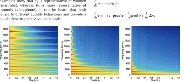
Simulations based on a modal decomposition have been proposed in [15] for realistic sound synthesis purposes, with the following sensible physical values: L¼0.5 m (bar length), w¼ 0.05 m (width), h¼0.0117 m (height), Y ¼ 2:13 + 1010_{Pa (Young's modulus)}

_ρ

_¼

1015 Kg m% 3 _{(purple wood density). When no damping is present,}

the first and last considered modes correspond to frequencies f1¼ 220 Hz and f12¼ 15 190 Hz, respectively.

As the damping coefficients are unknown, several physical orders of magnitude are presented: three sounds are synthesised and their respective spectrograms are presented inFig. 1. Qualita-tively, these examples show that b1 is representative of wooden

bar sounds (marimba), whereas b0 is more representative of

metallic bar sounds (vibraphone). It can be heard that both dampings give rise to different audible behaviours and provide a large set of sounds close to percussive bar sounds.

The spectrograms show how, on a practical example, such damping models can be used to improve the sound synthesis realism: both b0and b1are required.

For Rayleigh damping on conservative PDEs, analyzed in e.g. [18], a port-Hamiltonian formulation is available in e.g.[30]; we recall it here, for sake of clarity. In a simplified way, denoting v≔∂tu, the dynamics now reads

∂2_ttuþ yðvÞ þ ∂4 z4u ¼ 0;

with damping term (a polynomial of degree 1): yðvÞ≔b0vþ b1∂4z4v:

Classically, q≔∂2

z2u and p≔∂tu, with Hamiltonian H0≔12

RL

0ðq2þ p2Þ

dz. We can compute the variational derivatives

δ

qH0¼ q and

δ

pH0¼ p, and check d dt q p " # ¼ 0 ∂ 2 z2 %∂2 z2 0 " #

δ

qH0

δ

pH0 " # % 0 0 0 C # $

δ

qH0

δ

pH0 " # ;

(with C ¼ b0I þb1∂4z4) which has the desired ðJ % RÞ form, with J

skew-symmetric and R symmetric. In order to parametrize R ¼ GSGn , we define next G≔ 0₁ 0 ∂2 z2 " #

and S≔diagðb0I; b1IÞ;

which helps to describe the whole system, using the extended efforts and flows:

f f_p " # ¼ J G % Gn 0 " # e ep " # and ep¼ Sfp:

The feedback form which is obtained corresponds indeed to the damped dynamics:

_

X ¼ ðJ % GSGn

Þ

δ

XH0ðXÞ:

We now come to a non-linear system in 3 dimensions, for which the damping is fully structured: it perfectly fits into the dissipative pHs framework developed above.

Example 4 (Navier-Stokes equations). Following[28], we consider an irrotational and isentropic fluid, in a bounded domain

Ω

( R3. Using standard notations, the dynamical equations of the fluid can be written as d dt

ρ

¼ % divð

ρ

vÞ ð21Þ d dtv ¼ % ðv ) gradÞv % 1

ρ

grad p þ 1 Re

Δ

v; ð22Þ

Fig. 1. Rayleigh type dampings: spectrogram of ∂2

tuðt; LÞ. (left): b0¼ 4e % 2 and b1¼ 3e % 9 (SI), sounds like a metallic bar, (center): b0¼ 2e % 2 and b1¼ 5e % 8 (SI), sounds like

where pressure p is derivable from a potential energy density Uð

ρ

Þ, as p ¼

ρ

2_∂U=∂

_ρ

_{, and where v denotes the (vectorial) particle velocity.}

Here, Re is Reynolds number. Hence, with Hamiltonian H0≔ Z Ω 1 2

ρ

v ) v þ

ρ

Uð

ρ

Þ 7 8 dV; ð23Þ

we first compute the variational derivatives

δ

vH0¼

ρ

v;

and

δ

ρH0¼12v ) v þ hð

ρ

Þ;

with hð

ρ

Þ≔Uð

ρ

Þ þ

ρ

∂U=∂

ρ

being the enthalpy. Then, using the identity ðv ) gradÞv ¼ gradð1

2v ) vÞ which holds since rotðvÞ ¼ 0, we rewrite

Eqs.(21) and (22) as d dt

ρ

v # $ ¼ 0 % div % grad 0 " #

δ

ρH0

δ

vH0 " # % 0 0 0 C # $

δ

ρH0

δ

vH0 " # ;

with C ¼ % ð1=ReÞ

Δ

. It has the desired ðJ % RÞ form: J is skew-symmetric, since the formal adjoint of div is % grad, and R is symmetric and positive, since %

_Δ

is. More important, using the identity

_Δ

v ¼ gradðdivðvÞÞ which holds since % rotðrotðvÞ ¼ 0, the parametrization R ¼ GSGn

is very easily found to be G≔ 0 grad " # ; Gn ¼ ½0 % div'; and S≔1 ReI:

3.2.2. More general cases

Once again, for models of second order in time of the form(12), a sufficient condition for keeping the normal modes unaffected by the damping operator C, and proved in [5], is given by the commutation of the reduced operators, (including their domain). Condition (8) for finite-dimensional becomes (including the domains of these reduced operators)

½ ~C; ~K' ¼ 0: ð24Þ

Note that the original paper gives many counter-examples, either due to the structure of the operators, or their domains; an example is also provided.

As special cases, it proves very interesting to make a distinction between

1. polynomials, defined explicitly by: ~C≔Qð ~KÞ, such as Rayleigh damping when degðQ Þ ¼ 1, already discussed inSection 3.2.1, 2. rational functions, which can also be defined implicitly by:

Pð ~KÞ ~C≔Q ð ~KÞ,

3. irrational functions, such as ~C ¼ ~Kα, see e.g.Appendix A.2. In the sequel, we shall try to illustrate the latter two cases on worked-out examples. Let us start with a linear 1-D example with variable coefficients in space and rational damping.

Example 5 (Webster horn equation with rational damping). This model arising in musical acoustics is a wave equation, which has coefficients S(z) variable in space, it is first put in conservative form. The horn equation[21,3], also called the Webster equation [31], is a linear 1D model of axisymmetric acoustic pipes with a varying cross-section z↦SðzÞ ¼

π

RðzÞ2_{. For acoustic bells, this}

equation appeared to match with measurements choosing the space variable as the curvilinear abscissa which measures the length of the wall[14,16].

Denote

ρ

0 and P0 as the air density and the air pressure at

equilibrium, respectively. Denote

ρ

and p as their acoustic devia-tions for isentropic condidevia-tions. The wave equadevia-tions which govern the acoustic pressure p and the particle velocity v are given by,

respectively, 1 SðzÞ∂z½SðzÞ∂zpðz; tÞ'% 1 c2 0 ∂2tpðz; tÞ ¼ 0; ð25Þ ∂z 1 SðzÞ∂z½SðzÞvðz; tÞ' # $ %1 c2 0 ∂2_tvðz; tÞ ¼ 0; ð26Þ in the linear approximation, namely, for p , c2

0

ρ

where c0¼

ffiffiffiffiffiffiffiffiffiffiffiffiffiffiffiffi

γ

P0=

ρ

0

p

is the sound celerity and

γ

is the isentropic coefficient. The acoustic energy inside a pipe with length L is given by H0≔ Z L 0 1 2

ρ

0v2þ

ρ

0Uð

ρ

Þ 7 8 SðzÞ dz; ð27Þ where Uð

ρ

Þ ¼ ðc2 0=2

ρ

0Þ

ρ

2¼ ð

γ

P0=2

ρ

20Þ

ρ

2. Compared to (23), note

that the infinitesimal volume is dVðzÞ ¼ SðzÞ dz, that the kinetic energy is unchanged and that the potential energy is not the total internal energy of the gas, but is reduced to the acoustic part only. In acoustics, it is usually expressed as a function of p, namely,

ρ

0U ð

ρ

Þ ¼ p2=2

ρ

0c20. For z in ð0; LÞ, the corresponding

port-Hamiltonian system is described by d dt

ρ

v # $ ¼ 0 % 1 S∂zðS)Þ %∂z 0 2 4 3 5

δ

ρH0

δ

vH0 " # ; ð28Þ

where ð1=SÞ∂zðS)Þ stands for the divergence operator and∂zstands

for the gradient vector projected on ez. Moreover, operator J in(28)

is clearly skew-symmetric, w.r.t. the weighted scalar product ðv; wÞ≔RL

0vwSðzÞ dz.

Remark 6. In this 1D example, since the coefficients are space-varying, two distinct compound operators are to be found, depending on which variable we work on: either % SðzÞ% 1∂z½SðzÞ∂z:' or %∂z½SðzÞ% 1∂zðSðzÞ:Þ'.

Now, as far as damping is concerned, a first order rational function of operator

~

K≔ %SðzÞ% 1_∂

zðSðzÞ∂z:Þ ð29Þ

is being used for operator ~C. In order to be self-contained, let v≔∂tu and define y(v) as the solution to the following static PDE of

elliptic type:

a0y %a1S% 1∂zðS∂zyÞ ¼ b0v% b1S% 1∂zðS∂zvÞ; ð30Þ

where a1; b1Z0, and a₀; b040. With appropriate boundary con-ditions, this problem is well-posed, thanks to Lax–Milgram theo-rem. The positivity condition, RL

0yðzÞvðzÞ dz Z 0, can be checked

thanks to a spectral mapping theorem and f ðRþ_{Þ ( R}þ _where

f ðzÞ≔ðb0þ b1zÞ=ða0þ a1zÞ. But still, in this case, more precise results

can be proved. Setting

δ

≔b1a0% a1b0a0, two cases may occur, the

so-called ARMA model is of:

1. MA-type when

δ

40: First decompose the input v as v≔ða1=b1Þy þ w, then (30) implies ð

δ

=b1Þy ¼ b0w þ b1K~w, just

like Rayleigh damping on the new input w, which guarantees positivity:

ðy; vÞ ¼a1 b₁J yJ

2_{þ ðy; wÞ Z 0;}

since ð

δ

=b1Þðy; wÞ ¼ b0Jw J2þ b1ð ~Kw; wÞ Z0 (recall that ~K is a

positive self-adjoint operator).

2. AR-type when

δ

o0: First decompose the output y as y≔ðb1=a1Þv þ z, then (30) implies that a0z þ a1Kz ¼ % ð~

δ

=a1Þv,

guarantees positivity: ðy; vÞ ¼b1

a1JvJ

2_{þ ðz; vÞ Z0;}

since % ð

δ

=a1Þðz; vÞ ¼ a0Jz J2þ b1ð ~Kz; zÞZ0.

Remark 7. As very special case, one can consider the constant coefficient case SðzÞ ¼ S0, in which case an explicit solution can be

given, namely y ¼ ðb1=a1Þv % ð

δ

=a1Þexpð % jzj=ℓÞ⋆v, where ℓ ¼

ffiffiffiffiffiffiffiffiffiffiffiffi a1=a0

p

, which is an integral operator of convolution type, the convolution being bilateral in space.

Some decomposition of the type of those given inSection 2.2.2 could be copied and transferred to the infinite-dimensional set-ting; but so far, recasting this rational model in a port-Hamiltonian setting does not prove straightforward, even using the many extensions examined in[29, Section 4]. Hence, some more works could be done in order to be able to recast these more general integro-differential systems into a Dirac structure.

Let us finally turn to a more abstract case, which is neither polynomial nor rational.

Example 6 (Fractional Laplacian). Also of interest is the case of fractional Laplacian or bi-Laplacian (still with ideal boundary conditions), see [13,7,8] and references therein for this specific type of fractional damping model. More recently in[10], another interesting musical application makes use of C ¼ ð∂4

z4Þ

1=2_{, where}

K ¼ ∂4

z4, for the specific damping model of piano strings.

~

C ¼ ~Kα: ð31Þ

Remark 8. We refer toAppendix A.2for careful definitions of such non-rational functions of operators. In particular, ð∂4

z4Þ1=2a%∂2_z2

even with Dirichlet boundary conditions, and this can only be seen on the domain of the operators, or the specific decomposition on eigenfunctions.

The main idea behind this somewhat quite general damping model is to see the root locus it gives rises to: explicit analytical computations can be carried out on yðvÞ≔b0vþ bαð %

Δ

Þαv, but we

briefly show the root locus as a function of the

α

parameter in Figs. 2and3:

.

for 0o

α

o0:5, the dynamical system is a PDE of hyperbolic type, the roots are located on a curve in C with a so-called parabolic branch ImðsÞpð % ReðsÞÞνwith

ν

≔1=2

α

41,

.

for

α

¼ 0:5, the dynamical system is a PDE of parabolic type (the associated semigroup is analytic), the asymptote is a straight line (

ν

¼ 1),

.

for 0:5o

α

r1, the dynamical system is a PDE of parabolic or diffusive type, the roots are eventually located on R%_{, with}

only finitely many damped oscillating roots (located on a circle when

α

¼ 1, Rayleigh damping).

4. Conclusion and perspectives

We have looked for a structuration of the damping models which preserve the classical normal modes of the undamped structure, the Basile hypothesis. For discrete systems, or ODEs, the Caughey series has been put in the formalism of port-Hamiltonian system, the different cases have been examined and illustrated polynomial, rational function and even more general functions satisfying the positivity constraint. For continuous sys-tems, or PDEs, the general ideas behind Caughey series have also been put into the port-Hamiltonian setting, at least formally, and a few interesting examples have been treated.

Fig. 2. From left to right: α ¼ 0 fluid; α ¼ 0:1, 0.25, 0.4 PDE of hyperbolic type.

Moreover, many points are to be looked at carefully, in the continuation of this preliminary work on structuration of damp-ing, such as

.

For the PDE case, ports at the boundaries of the spatial domain must definitely be taken into account, see e.g.[30] and [19, Chapters 9 and 10].

.

_{How to use these models for the purpose of identification of}

damping parameters? Is an inverse problem possible, tractable in the context of structured damping?

.

Possibility to adapt to nonlinear models with non-quadratic Hamiltonian? Could the Hessian functional help to define the different terms, such as K(q) and M(p)? See e.g.[9, Section 2.3].

.

Use some operational calculus on non-normal operators? Think of Riesz basis as directly related to Hilbert basis (following e.g. [20]) and then use this as a foundation for operational calculus: is that a too naive idea? Its interest is that it seems to be tractable, but to what extent, and is there a solid theory beyond that? See e.g.[17,27].

.

In the previous case, how does the positivity constraint translate? Into a positive real condition, such as Reðf ðzÞÞ Z 0 for ReðzÞ4 0?

.

For PDEs, go to the case when the physical domain is of dimension d¼2 or 3: things become much more intricate, new operators pop up, such as div and % grad, which are adjoints one of another, but % divðgradÞ is a scalar operator %

Δ

acting on functions, whereas % gradðdivÞ is a vector-valued operators acting on vector fields (already when d¼1, the non-commutativity has been noticed inRemark 6when the coeffi-cients are space-varying).

And, last but not least, an objection could very much be raised before going on: what is the real interest, and on what physical ground, do we look for normal modes in damped structures? Different answers are possible: one could argue that eigenvalues are affected at the first order when a slight damping is applied, whereas eigenvectors or eigenfunctions are only moved up to the second order of the damping parameter. Moreover, for many physical problems, refined damping models are not available. For instance, in applications such as inExample 3(see e.g.[6]), an engineering approach is often used, which consists in computing the modal decomposition of the con-servative problem and introducing, a posteriori, a specific damping for the dynamics of each mode according to some heuristics. Damping models that preserve the eigenspaces of the conservative problem exactly address this issues but, in an intrinsic way, that is, without having to derive the eigenstructure. This gives both a formal frame-work and define an equivalence class of damped models.

Finally, pHs formalism proves most useful when modelling damp-ing for PDEs: when non-ideal boundary conditions are present, not simply Dirichlet or Neumann, such as Robin type or more general impedance boundary conditions, there is a need to clarify the under-lying structure, which could very much be given, almost for free, by the port variables in the pH framework: this is, at the best of our knowledge, one of the most important reason to turn to pHs for PDEs in order to build and define coherent damping models.

Acknowledgments

Both authors would like to thank the two anonymous reviewers, who carefully read the original submission, made useful comments, and greatly helped to enhance the final version of the paper; they are gratefully acknowledged.

The first author would like to thank Prof. J. Kergomard for fruitful discussion on the subject of gyroscopic terms for ODEs,

first giving the right name to this term, then giving the example of Coriolis effect in solid mechanics, seeSection 2.1.2.

The first author would like Prof. S. De Bièvre for the nice talk on Abraham–Lorentz model and the Hamiltonian framework, see Section 2.1.2.

The first author would like to thank Prof. L. Jezequel for fruitful discussion on the subject of gyroscopic terms for PDEs, and mentioning the example of fluid mechanics in a duct with convection, seeSection 3.1.2.

The first author would like to thank Prof. B. Maschke for fruitful discussion on the parametrization of implicit port-Hamiltonian systems.

Appendix A

A part of this technical presentation on fractional powers of matrices and operators is borrowed from[23], see also[25]for a clear and concise course with many examples of operators and spectra.

A.1. Fractional powers of matrices

We recall the Spectral Theorem for symmetric real-valued matrices: if A ¼ ATAM_n+nðRÞ, then there exist a diagonal matrix

Λ

and an orthogonal matrix P, (i.e. PT_{P ¼ I}

n), such that A ¼ P% 1

Λ

P.

Then, for the fractional power of a symmetric matrix, two cases may occur:

1. if A ¼ AT

40, i.e. A is positive definite, then one can uniquely define A%β_{¼ P}% 1

_Λ

%β_{P, with}

_Λ

%β_{¼ diagð}

_λ

%β

1 ;…;

λ

%β

n Þ, since

λ

i40. 2. if A ¼ AT_Z

0, i.e. A is positive, then one can uniquely define Aα¼ P% 1

Λ

αP, with

Λ

α¼ diagð

λ

α1;…;

λ

α

nÞ, since

λ

iZ0.

A.2. Fractional powers of operators

A key point is the compactness property: when it is present, this property enables to write down things into series instead of finite sums (with the celebrated sine, cosine or Fourier series on L2ðIÞ, where I is a bounded interval), and this applies both to bounded and unbounded operators in fact. When it is not present, general integrals instead of series have to be considered: we recall the celebrated Fourier transform on L2_ðRÞ.

A.2.1. Fractional powers for operators with a compactness property In an infinite-dimensional setting, things are much more complicated: we begin with the case of bounded operators.

Bounded operators: Following standard theory, if K is a compact and symmetric operator on a Hilbert space H, using the Spectral Theorem, we get a spectral mapping theorem of the form above: 1. if K ¼ KT_{40, i.e. K is positive definite, then one can uniquely}

define K%β_{¼ P}% 1

_Λ

%β

P, with

Λ

%β¼ diagðk_n%βÞ_{n A N}, since kn40; this unbounded operator is defined on a domain DðK%β_{Þ, see}

Section A.2.1.

2. if K ¼ KTZ0, i.e. K is positive, then one can uniquely define Kα¼ P% 1

Λ

αP, with

Λ

α¼ diagðkα_nÞn A N, since knZ0.

The transform P is unitary on H, and the eigenvalues of K consist in a sequence of positive real numbers knwhich converge towards 0.

Unbounded operators: Now if A is unbounded on H, with dense domain D(A) in H, self-adjoint, positive, and has compact resolvent, then the previous setting can be applied to Kρ¼ ð

ρ

I %AÞ% 1 for

ρ

A

ρ

_{ðAÞ, the resolvent set of A; in particular the eigenvalues of A} form a discrete sequence

λ

nof positive real numbers, which grows

towards infinity. When

λ

¼ 0 is not an eigenvalue of Kρ, the

eigenvectors ðenÞn A Nof Kρ form a Hilbert basis of H, and we get

the spectral theorem: 8

φ

AH;

φ

¼ ∑

n A N

ð

φ

; enÞen;

with the energy identity J

φ

J2H¼∑n A Njð

φ

; enÞj2. And for any

γ

40, we can define the fractional power of A as follows:

Aγ

φ

¼ ∑

n A N

λ

γ

nð

φ

; enÞen;

provided

φ

ADðAγÞ, where DðAγÞ ¼

φ

AH; ∑ n A N

λ

2γ n jðen;

φ

Þj2o1 9 : : This is indeed the case for A ¼ % ∂2

x2 on the bounded interval

I ¼ ð0; 1Þ, with Dirichlet (D) or Neumann (N) boundary conditions at each end:

.

D–D case:

λ

n¼ n2

π

2and enpsin ðn

π

xÞ for nZ 1,

.

_{D–N case:}

λ

n¼ ðn þ12Þ2

π

2and enpsin ððnþ1₂Þ

π

xÞ for nZ 0,

.

_{N–D case:}

λ

n¼ ðn þ1₂Þ2

π

2and enpcos ððnþ1

2Þ

π

xÞ for n Z 0,

.

N–N case:

λ

n¼ n2

π

2 and enpcos ðn

π

xÞ for nZ 0, (note that

λ

¼ 0 is indeed an eigenvalue).

Also useful is the case of Aper¼ %∂2_x2 with periodic boundary

conditions on I, leading to 1.

λ

0¼ 0 and e0¼ 1,

2. for nZ 1,

λ

n¼ 4

π

2n2, the 2-dimensional eigenspace being

spanned by orthogonal eigenvectors en;1pcos ð2

π

nxÞ and en;2psin ð2

π

nxÞ;

in which case we recover the celebrated Fourier series decom-position.

A.2.2. Fractional powers for operators without a compactness property

Consider A ¼ % ∂2

x2on the unbounded interval R, we know from

Fourier analysis in H ¼ L2_{ðRÞ that this operator can be diagonalized}

as follows, with P ¼ F : L2_ðR

xÞ-L2ðRξÞ, the unitary Fourier

trans-form, and P% 1_{¼ F}% 1_:L2_ðR ξÞ-L2ðRxÞ: ^ A : L2ðRξÞ-L2ðRξÞ ^

φ

↦₄

_π

2

_ξ

2

_φ

^_; ð32Þ

on the domain Dð ^AÞ ¼ L2;2ðRξÞ, where we have set

L2;sðRξÞ≔

φ

^AL2ðR_ξÞ; Z R ð1 þ 4

π

2

_ξ

2 Þsj ^

φ

j2d

ξ

o1 9 : :

For

γ

40, it is then not difficult to define the fractional power of A in the following way: Aγ¼ P% 1A^γP, where

^ Aγ:L2_ðR

ξÞ-L2ðRξÞ

^

φ

↦_ð4

_π

2

_ξ

2_Þγ

_φ

^_; ð33Þ

on the domain Dð ^AγÞ ¼ L2;2γðRξÞ. We can see here that since the

compactness is lost, no Hilbert basis will help diagonalize the operator; even though the space L2_ðR

xÞ is separable, meaning it

has a countable family which is everywhere dense, such as the Hermite functions.

References

[1]S. Adhikari, Damping modelling using generalized proportional damping, J. Sound Vib. 293 (2006) 156–170.

[2]V. Arnold, Lectures on Partial Differential Equations. Universitext, Springer, 2004.

[3]D. Bernoulli, Physical, mechanical and analytical researches on sound and on the tones of differently constructed organ pipes, Mém. Acad. Sci. (Paris), 1762 (in French).

[4]T.K. Caughey, Classical normal modes in damped linear dynamic systems, Trans. ASME, J. Appl. Mech. 27 (1960) 269–271.

[5]T.K. Caughey, M.E.J. O'Kelly, Classical normal modes in damped linear dynamic systems, Trans. ASME, J. Appl. Mech. 32 (1965) 583–588.

[6]R. Causse, J. Bensoam, N. Ellis, Modalys, a physical modeling synthesizer: more than twenty years of researches, developments, and musical uses, J. Acoust. Soc. Am. 130 (2011) 2365. (abstract).

[7]S.P. Chen, R. Triggiani, Proof of two conjectures by G. Chen and D. L. Russell on structural damping for elastic systems, in: Approximation and Optimization (Havana, 1987), vol. 1354, 1988, pp. 234–256.

[8]S.P. Chen, R. Triggiani, Proof of extensions of two conjectures on structural damping for elastic systems, Pac. J. Math. 136 (1) (1989) 15–55.

[9]V. Duindam, A. Macchelli, S. Stramigioli, H. Beruyninckx (Eds.), Modeling and Control of Complex Physical Systems. The Port-Hamiltonian Approach, Springer Verlag, 2009.

[10]K. Ege, La table d'harmonie du piano - Etudes modales en basses et moyennes fréquences (Thèse de doctorat), Ecole Polytechnique, 2009.

[11] M. Géradin, D. Rixen, Mechanical Vibrations: Theory and Application to Structural Dynamics, John Wiley, 1997.

[12]K.F. Graff, Wave Motion in Elastic Solids, Dover, 1975.

[13]S. Hansen, Optimal regularity results for boundary control of elastic systems with fractional order damping, ESAIM: Proc. 8 (2000) 53–64.

[14]Hélie Thomas, Mono-dimensional models of the acoustic propagation in axisymmetric waveguides, J. Acoust. Soc. Am. 114 (2003) 2633–2647. [15]T. Hélie, D. Matignon, Damping models for the sound synthesis of bar-like

instruments, in: 7th International Conference on Systemics, Cybernetics and Informatics, Orlando, Florida, 2001, pp 541–546 (invited session).

[16]Hélie Thomas, Hézard Thomas, Mignot Rémi, Matignon Denis, On the 1D wave propagation in wind instruments with a smooth profile, in: Forum Acusticum, vol. 6, Aalborg, Danemark, Juillet, 2011, pp. 1–6.

[17] A. Intissar, Analyse Fonctionnelle et théorie spectrale pour les opérateurs compacts non auto-adjoints, Cépaduès, 1997.

[18]B. Jacob, C. Trunk, M. Winklmeier, Analyticity and Riesz basis property of semigroups associated to damped vibrations, J. Evol. Equ. 8 (2) (2008) 263–281.

[19]B. Jacob, H.J. Zwart, Linear Port-Hamiltonian Systems on Infinite-dimensional Spaces, Series: Operator Theory: Advances and Applications, Subseries: Linear Operators and Linear Systems, vol. 223, Birkhäuser, 2012.

[20] J. Kergomard, V. Debut, D. Matignon, Resonance modes in a 1-D medium with two purely resistive boundaries: calculation methods, orthogonality and completeness, J. Acoust. Soc. Am. 119 (2006) 1356–1367.

[21]J.L. Lagrange, Nouvelles recherches sur la nature et la propagation du son, Misc. Taur. (Mélanges Phil. Math., Soc. Roy. Turin) 1 151–316.

[22] Y. Le Gorrec, H. Zwart, B. Maschke, Dirac structures and Boundary Control Systems associated with Skew-Symmetric Differential Operators, SIAM J. Control Optim. 44 (5) (2005) 1864–1892.

[23] D. Matignon, Diffusive representations for fractional Laplacian: systems theory framework and numerical issues, Phys. Scr. T136 (2009) 014009 (6 p.) 〈http:// oatao.univ-toulouse.fr/3889/〉.

[24] D. Matignon, T. Hélie, On damping models preserving the eigenfunctions of conservative systems: a port-Hamiltonian perspective. In: IFAC Conference on Lagrangian and Hamiltonian Methods and Nonlinear Control (LHMNLC'12) August 29–31, 2012, Bertinoro, Italy (invited session).

[25] A.W. Naylor, G.R. Sell, Linear Operator Theory in Engineering and Science, Applied Mathematical Sciences Series, vol. 40, Springer Verlag, 1982. [26] J.W.S. Rayleigh, Theory of Sound, 2nd edition, Dover, New York, 1896,

Reprinted 1945.

[27] L.N. Trefethen, M. Embree, Spectra and Pseudospectra: The Behavior of Nonnormal Matrices and Operators, Princeton University Press, 2005. [28] A. van der Schaft, B. Maschke, Fluid Dynamical Systems as Hamiltonian

Boundary Control Systems, Memorandum 1575, University of Twente, 2001. [29] A. van der Schaft, B. Maschke, Port-Hamiltonian systems: network modeling

and control of nonlinear physical systems, in: Advanced Dynamics and Control of Structures, CISM International Centre for Mechanical Sciences, vol. 444, 2004, Springer.

[30] J. Villegas, Y. LeGorrec, H. Zwart, B. Maschke, Boundary control for a class of dissipative differential operators including diffusion systems, in: Mathema-tical Theory of Networks and Systems (MTNS), MoP06.4. Kyoto, Japan, 2006, pp. 297–304 (invited session).

[31]A.G. Webster, Acoustical impedance, and the theory of horns and of the phonograph, Proc. Natl. Acad. Sci. USA 5 (1919) 275–282. (Errata, Proc. Natl. Acad. Sci. USA 6 (1920) 320).