2013 — Experimental process development and aerospace alloy formability studies for hydroforming

ÉCOLE DE TECHNOLOGIE SUPÉRIEURE UNIVERSITÉ DU QUÉBEC

MASTER’S THESIS PRESENTED TO ÉCOLE DE TECHNOLOGIE SUPÉRIEURE

IN PARTIAL FULFILLEMENT OF THE REQUIREMENTS FOR MASTER’S DEGREE IN MECHANICAL ENGINEERING

M. Eng.

BY

Saeed MOJARAD FARIMANI

EXPERIMENTAL PROCESS DEVELOPMENT AND AEROSPACE ALLOY FORMABILITY STUDIES FOR HYDROFORMING

MONTREAL, DECEMBER 18 2013

© Copyright reserved

It is forbidden to reproduce, save or share the content of this document either in whole or in parts. The reader who wishes to print or save this document on any media must first get the permission of the author.

BOARD OF EXAMINERS

THIS THESIS HAS BEEN EVALUATED BY THE FOLLOWING BOARD OF EXAMINERS

Mr. Henri Champliaud, Thesis Supervisor

Mechanical engineering department at École de technologie supérieure

Mr. Javad Gholipour Baradari, Thesis Co-supervisor

National Research Council, Institute for Aerospace Research, Aerospace Manufacturing Technologies Center

Mr. Van Ngan Lê, President of the Board of Examiners

Mechanical engineering department at École de technologie supérieure

Mr. Mohammad Jahazi, External Evaluator

Mechanical engineering department at École de technologie supérieure

Mr. Jean Savoie, External Evaluator Pratt & Whitney Canada

THIS THESIS WAS PRENSENTED AND DEFENDED

IN THE PRESENCE OF A BOARD OF EXAMINERS AND PUBLIC DECEMBER 02 2013

To

The love of my life

Vida

ACKNOWLEDGMENT

I would like to thank my supervisor, Professor Henri Champliaud for his support and invaluable trust throughout this master program. I want to thank him for the opportunity that he gave to me and for all his supports. Those two and a half years have been great and full of knowledge.

I would like to extend my special thanks to my co-supervisor Dr. Javad Gholipour Baradari from National Research Council of Canada (NRC)-Aerospace for his helpful and insightful advice as well as his constant availability. Our many discussions helped me improve my critical thinking abilities, build my profile as a researcher and a whole lot more.

I would like to thank Dr. Van Ngan Lê and Dr. Mohammad Jahazi, professors at ETS, for accepting to be part of my board of examiners.

I also sincerely thank to Dr. Jean Savoie from Pratt & Whitney Canada for his enthusiastic support and pertinent suggestions all along the Project. This work was made possible by the financial support provided by Pratt & Whitney Canada, NRC-Aerospace, Natural Sciences and Engineering Research Council of Canada (NSERC) and Consortium de recherche et d'innovation en aérospatiale au Québec (CRIAQ).

I am particularly grateful to my friends and colleagues who put up with me during the hard and the joyful times.

My special thanks go to my parents; you supported me throughout my studies and helped me achieve what I have accomplished so far. It would not be possible for me to accomplish all these without your help and encouragement.

Last but not least, I would like to send my special thanks to Vida for always being there for me; I will always be grateful for your patience, love and support.

EXPERIMENTAL PROCESS DEVELOPMENT AND AEROSPACE ALLOY FORMABILITY STUDIES FOR HYDROFORMING

Saeed MOJARAD FARIMANI RÉSUMÉ

Dans le procédé d’hydroformage, la pression d’un fluide est utilisée pour déformer plastiquement un tube paroi mince à l’intérieur d’une matrice fermée afin de remplir la cavité de la matrice. L’hydroformage des tubes possède de nombreux avantages qui rendent ce procédé très intéressant pour plusieurs industries telles que l’automobile et l’aérospatiale. Mais, à cause de différents facteurs tels que la formabilité des matériaux, l’ordre et les séquences du chargement (force de compression axiale et pression interne pendant le procédé), la géométrie de l’outil et la friction, c’est un procédé de mise en forme assez complexe. Ainsi, la simulation par éléments finis combinée à des méthodes d’optimisation peuvent réduire significativement le coût de l’approche “Essai – Erreur” utilisée dans les méthodes conventionnelles de mise en forme. Dans ce mémoire, pour étudier les effets de différent paramètres tels que les conditions de friction, l’épaisseur du tube et la compression axiale sur la pièce finale, des essais d’hydroformage de tube ont été menés en utilisant une matrice de forme ronde à carrée. Les expériences ont été effectuées sur des tubes d’acier inoxydable 321 de 50.8 mm (2 in) de diamètre et deux différentes épaisseurs ; 0.9 mm et 1.2 mm. L’historique du chargement a été enregistré avec le système d’acquisition de la presse. Un système de mesure de déformation automatique, Argus, a été utilisé pour mesurer les déformations sur les tubes hydroformés. Les données collectées à partir des essais initiaux ont été utilisées pour comparer avec les simulations. Le procédé a été simulé et optimisé à partir des logiciels Ls-Dyna et Ls-Opt, respectivement. Les variations de déformations et d’épaisseurs mesurées à partir des expériences ont été comparées aux résultats de la simulation par éléments finis dans les zones critiques. La comparaison des résultats de la simulation et des expériences sont en bon accord indiquant que l’approche peut être utilisée pour prédire la forme finale et les variations d’épaisseurs de pièces hydroformées pour des applications aérospatiales.

Mots-clés: Hydroformage de tube; analyse par éléments finis, optimisation, alliages aéronautiques

EXPERIMENTAL PROCESS DEVELOPMENT AND AEROSPACE ALLOY FORMABILITY STUDIES FOR HYDROFORMING

Saeed MOJARAD FARIMANI ABSTRACT

In tube hydroforming process, a pressurized liquid is used to expand a thin walled tube inside a closed die in order to fill the die cavity. Tube hydroforming has many advantages that make it interesting for different industries such as automotive and aerospace, but due to the effects of different factors, such as formability of the material, load path (end feeding force and internal pressure during the process), tool geometry and friction, it is a quite complex manufacturing process. Therefore, finite element simulation along with optimization methods can significantly reduce the cost of trial and error approach used in conventional manufacturing methods. In this work, to investigate the effects of different process parameters such as friction condition, tube thickness and end feeding on the final product, tube hydroforming experiments were performed using a round to square-shape die. Experiments were performed on stainless steel 321 tubes with 50.8 mm (2 in) diameter and two different thicknesses; 0.9 mm and 1.2 mm. Experimental load paths were obtained via the data acquisition system of the hydroforming press, which is fully instrumented. An automated deformation measurement system, Argus, was used to measure the strains on the hydroformed tubes. Data collected from the initial experiments were used to simulate and then optimize the process. The process was simulated and optimized using Dyna and Ls-Opt software, respectively. Strains and thickness variations measured from experiments were compared to FE simulation results at critical sections. The comparison of the results from FE simulations and experiments were in good agreement, indicating that the approach can be used for predicting the final shape and thickness variations of the hydroformed parts for aerospace applications.

TABLE OF CONTENTS

Page

INTRODUCTION ... 1

CHAPTER 1 LITERATURE REVIEW ... 5

1.1 EFFECTIVE PARAMETERS IN THF PROCESS ... 5

1.1.1 Effect of material properties ... 5

1.1.2 Effect of geometrical factors ... 11

1.1.3 Effect of loading path ... 12

1.1.4 Effect of friction and lubrication ... 15

1.2 INSTABILITIES AND FAILURES ... 18

1.3 FINITE ELEMENT MODELING ... 21

1.4 PROCESS OPTIMIZATION ... 23

CHAPTER 2 METHODOLOGY ... 27

2.1 FINITE ELEMENT MODEL (FEM) ... 27

2.1.1 Contact condition ... 29

2.1.2 Load path simulation... 30

2.1.3 Material model ... 31 2.1.4 Time scaling ... 32 2.1.5 Spring back ... 32 2.2 EXPERIMENTAL SETUP ... 33 2.2.1 Die ... 34 2.2.2 Plungers... 35

2.2.3 Expansion measurement unit ... 35

2.2.4 Tube preparation ... 37

2.2.5 Hydroforming ... 40

2.2.6 Strain and thickness measurement ... 43

2.3 OPTIMIZATION ... 45

3.1 EXPERIMENTAL RESULTS ... 49

3.2 FEM VERIFICATION ... 53

3.2.1 Material properties ... 53

3.2.2 Different element types ... 57

3.2.3 Strain distribution... 62 3.3 EFFECT OF LUBRICATION ... 66 3.4 OPTIMIZATION ... 72 CONCLUSION ... 77 RECOMMENDATIONS ... 79 APPENDIX A ... 81 APPENDIX B ... 85 APPENDIX C ... 89 APPENDIX D ... 91 APPENDIX E ... 95 APPENDIX F... 99 APPENDIX G ... 101 APPENDIX H ... 103 APPENDIX I ... 105

LIST OF TABLES

Page

Table 2.1 Material properties of the SS321 tubes ...31

Table 2.2 Optimization settings in LS-OPT...48

Table 3.1 Optimization results for 0.9 mm tube thickness ...73

LIST OF FIGURES

Page

Figure 0.1 Typical tube hydroforming process ...2

Figure 1.1 Tensile test specimens cut from the tube ...6

Figure 1.2 The schematic of free expansion test ...7

Figure 1.3 Wall thickness distribution for different n-values ...9

Figure 1.4 The effect of n-value and K-value on bursting pressure ...9

Figure 1.5 The effect of r-value on bursting pressure in THF process ...10

Figure 1.6 The effect geometrical parameters on bulge height in T-shape THF ...11

Figure 1.7 Schematic of single and multiple strokes axial feed paths in THF ...14

Figure 1.8 (A) Pressure advanced, (B) Linear, and (C) Feed advanced loading paths ...14

Figure 1.9 Friction zones in THF ...16

Figure 1.10 (a) Corner fill and (b) Pear-shaped expansion test for evaluate the lubricants in expansion zone ...17

Figure 1.11 Different failure mode in THF process ...19

Figure 1.12 Process windows for THF process ...19

Figure 1.13 A typical FLD ...20

Figure 1.14 (a) Direct and (b) approximate optimisation ...25

Figure 2.1 Symmetry planes ...28

Figure 2.2 (a) shell and (b) solid FEM ...29

Figure 2.3 A typical end feed and internal pressure versus time curve ...30

Figure 2.4 True stress-strain curves for tubes with (a) 0.9 mm and (b) 1.2 mm thicknesses ...32

Figure 2.6 Round-to-square die Set ...34

Figure 2.7 Plungers setup ...35

Figure 2.8 Expansion measurement unit (a) initial stage (b) final stage ...36

Figure 2.9 Setup of the expansion measurement units ...37

Figure 2.10 The ultrasonic thickness measurement device (38DL Plus) ...38

Figure 2.11 Circumferential thickness variation for tubes with (a) 0.9 mm (b) 1.2 mm thickness (dimensions in mm)...38

Figure 2.12 Pattern produced on the tube surface ...39

Figure 2.13 Free end load path for tube with 0.9 mm thickness ...42

Figure 2.14 Loading paths for tubes with (a) 0.9 mm and (b) 1.2 mm thickness ...42

Figure 2.15 Camera movement around measuring object ...43

Figure 2.16 Pictures from different views of the deformed tube ...44

Figure 2.17 Thickness measurement regions ...45

Figure 2.18 Design variables (P and F) in optimum loading path ...46

Figure 2.19 FLD for SS321tubes with 0.9 mm and 1.2 mm thicknesses ...47

Figure 3.1 Expansion in tubes with (a) 0.9 mm and (b) 1.2 mm thickness ...50

Figure 3.2 Thickness variation of tubes with (a) 0.9 mm and (b) 1.2 mm thickness ...51

Figure 3.3 Tube position after hydroforming ...52

Figure 3.4 Tube expansion in 0.9 mm thick tube (a) free end (b) load path 1 (c) load path 2 and (d) load path 3 ...54

Figure 3.5 Expansion of the tubes with 1.2 mm thickness (a) free end (b) loading path 1 (c) loading path 2 and (d) loading path 3 ...55

Figure 3.6 Thickness variation in tubes with 0.9 mm thickness (a) free end (b) loading path 1 (c) loading path 2 and (d) loading path 3 ...56

Figure 3.7 Thickness variation in tubes with 1.2 mm thickness (a) free end (b) loading path 1 (c) loading path 2 and (d) loading path 3 ...57

Figure 3.8 Expansion of the tubes with different element types for 0.9 mm thick tube (a) free end (b) loading path 1 (c) loading path 2 and

(d) loading path 3 ...58 Figure 3.9 Expansion of the tubes with different element types for 1.2 mm

thick tube (a) free end (b) loading path 1 (c) loading path 2 and

(d) loading path 3 ...59 Figure 3.10 Thickness variation in tubes with 0.9 mm thickness (a) free end

(b) loading path 1 (c) loading path 2 and (d) loading path 3 ...60 Figure 3.11 Thickness variation in tubes with 1.2 mm thickness (a) free end

(b) loading path 1 (c) loading path 2 and (d) loading path 3 ...61 Figure 3.12 Major strain distribution on the surface of the tube for loading path 1

(0.9 mm) (a) simulation (b) experiment ...63 Figure 3.13 Minor strain distribution on the surface of the tube for loading path 1

(0.9 mm) (a) simulation (b) experiment ...63 Figure 3.14 Major strain distribution on the surface of the tube for loading path 3

(0.9 mm) (a) simulation (b) experiment ...64 Figure 3.15 Minor strain distribution on the surface of the tube for loading path 3

(0.9 mm) (a) simulation (b) experiment ...65 Figure 3.16 Strain distribution for mid length cross section of 0.9 mm tubes

hydroformed with (a) loading path 1 (b) loading path 3 ...66 Figure 3.17 Expansion for tubes with different lubricants (a) 0.9 mm and

(b) 1.2 mm thick tubes ...68 Figure 3.18 Thickness variation of tubes with different lubricants (a) 0.9 mm

and (b) 1.2 mm thick tubes ...69 Figure 3.19 Tube expansion curves for different COFs (a) 0.9 mm

(b) 1.2 mm thick tubes ...70 Figure 3.20 Tube thickness variation for different COFs (a) 0.9 mm

(b) 1.2 mm thick tubes ...71 Figure 3.21 Loading paths for tubes with (a) 0.9 mm (b) 1.2 mm thicknesses ...73 Figure 3.22 Tube expansion curves for optimum loading paths (a) 0.9 mm

Figure 3.23 Tube thickness variations for optimum loading paths (a) 0.9 mm

LIST OF ABREVIATIONS THF Tube Hydroforming

FEA Finite Element Analysis FEM Finite Element Model SS321 Stainless Steel 321 COF Coefficient of Friction n-value Strain Hardening Exponent r-value Material Anisotropy

HPTH High Pressure Tube Hydroforming LPTH Low Pressure Tube Hydroforming FLD Failure Limit Diagram

FLC Failure Limit Curve ESD Effective Strain Diagram FLSD Forming Limit Stress Diagram FLSC Forming Limit Stress Curve

XSFLD Extended Stress Based Forming Limit Diagram XSFLC Extended Stress Based Forming Limit Curve GA Genetic Algorithms

NRC National Research Council of Canada Tshell element Thick shell element

INTRODUCTION

By increasing demand from different transportation industries for producing low weight and safe structures, manufacturers have to use cutting edge materials and manufacturing techniques to make lightweight, reliable and, cost-efficient structures with consistent quality. During last decade, Tube hydroforming (THF) process has emerged as a suitable manufacturing process to produce complex shapes with minimum dimensional variations and fewer secondary operations. Hence, having a good insight into this relatively new metal forming process is quite important. This chapter will put forward a brief introduction about THF process and its pros and cons. Then the objectives of the present study will be presented followed by the thesis outline.

Hydroforming concept

The fundamentals of hydroforming were established in 1940s when Grey et al. used internal pressure and axial load to investigate the production of seamless copper fittings with T protrusions (Alaswad, Benyounis et Olabi, 2012). The first use of the hydroforming process in mass production dates back to about 40 years ago when it was used to manufacture copper tubes for sanitary industry. By growing demand for more efficient manufacturing methods, hydroforming has widely opened its way in various industries such as automotive and aerospace as an advanced manufacturing technology and as an alternative for conventional production processes such as stamping and welding. Exhaust manifolds, exhaust pipes, radiator enclosures, frame rail, chassis and engine cradles are some of the most well-known hydroformed parts in automotive industries (Dohmann et Hartl, 1997). Although different classifications have been made by different researchers (Siegert et al., 2000; Zhang, 1999), hydroforming can be classified into two main categories, sheet hydroforming and tube hydroforming (Koç et Altan, 2001). Despite some differences between these two processes, the basic principle remains the same: using an internal fluid pressure to form a blank material. The focus of the present study is on the tube hydroforming process.

Tube hydroforming

Tube hydroforming is a metal forming process in which a tube is formed into complex shapes inside a closed die using simultaneously an internal pressure and axial loads at the tube ends. Figure 0.1 shows the sequence of a typical THF process. The process begins with placing the blank tube, which has been cut to the appropriate length, inside the die cavity (Figure 0.1a). Then the die closes and the plungers move towards the tube ends to press against the ends of the tube and seal it (Figure 0.1b). In the next step, the liquid is pressurized inside the tube and axial force is applied to the tube ends to form the tube into the die shape (Figure 0.1c).

Figure 0.1: Typical tube hydroforming process (Guan, Pourboghrat et Yu, 2006)

Thanks to the recent technological improvements, especially in control systems, tube hydroforming of massive parts has become a viable technique during the last two decades. Tube hydroforming offers many advantages in comparison with traditional manufacturing methods (Ahmetoglu et Altan, 2000; Dohmann et Hartl, 1996; 1997) such as:

1) weight reduction of the final part through tailoring of the section design and tube geometry.

2) decreasing the production costs by eliminating the secondary operations, such as welding/trimming, and reduction in material waste.

3) reducing the labor costs through part consolidation, tighter tolerances and reduced spring back that increases production repeatability.

4) increasing structural strength through optimized section design.

With its unique advantages, THF have some drawbacks (Ahmetoglu et Altan, 2000; Ahmetoglu et al., 2000; Koç, 2008; Koç et al., 2000; Zhang, 1999) such as:

1) slow cycle time; 2) expensive equipments;

3) insufficient existing knowledge base for process and tool design.

To fill this lack of knowledge and to improve and optimise THF process, many studies have been carried out up to now. In the next chapter a thorough review of the past research will be presented.

Research objectives and methodology

In this thesis, we will follow two main goals. The first one is to study the effect of different parameters like material properties, tube thickness, load path and friction condition on THF process. To study these parameters, a finite element model (FEM) was developed using 3D non linear LS-DYNA as the solver. For validating the FEM, a series of experiments have been performed using stainless steel 321 (SS321) with two different thicknesses; 0.9 mm and 1.2 mm. A fully instrumented hydroforming press was used to apply different loading paths during the experiments. A laser measurement system was mounted on the press to measure tube expansion during the hydroforming process. Furthermore, the strains on the surface of the deformed tubes were measured using an automated deformation measurement system

(ARGUS®). In the end, the results from finite element analysis (FEA) and the experiments were compared to check the reliability of the FEM.

The second objective of this project was to predict the optimum loading path for the tube hydroforming process using LS-Opt software. The objectives of the optimization procedure were to maximise the expansion of the tubes with minimum wall thickness variation.

Thesis outline

This thesis will be presented in the following chapters:

In chapter 1 a thorough literature review on FEA, parameters that affect the THF process and optimisation procedures will be presented. In chapter 2 the FEM, the experimental and the optimization approach used for this study will be explained. In Chapter 3 the results that have been obtained from the FEA and experiments will be presented and discussed. And finally, chapter 4 summarizes the conclusions of this research and offers some recommendations for future works.

CHAPTER 1

LITERATURE REVIEW

This chapter presents an overview of available published results concerning various aspects of THF. First, the design parameters and process condition that affect the forming process is presented. After that, the failure modes that usually occur during the process and the technique to predict and avoid these failure modes are discussed. Finally, an overview on the optimisation techniques used to improve the quality of final part is presented.

1.1 Effective parameters in THF process

The end result of a THF process is highly relied on different parameters like the tube material properties, the geometrical parameters of the tube and die such as corner radius of the die, tube length, tube diameter and tube thickness and the process parameters such as load path and friction condition. The effect of each parameter should be taken into consideration to produce a sound product. Many researchers have studied the effects of these parameters in THF process up to now. In this section a review on these researches is presented

1.1.1 Effect of material properties

Material property plays an important role in THF process. It can affect the magnitude of the process parameters such as the internal pressure and the axial load as well as the tube expansion and the thickness variation (Ahmetoglu et Altan, 2000). On the other hand, as mentioned before, FEA has become a common tool in investigating the THF process and it demands reliable material parameters such as elastic module, yield strength, ultimate tensile strength and anisotropy to simulate the forming process of the tube accurately. However, there is not a standard procedure for extracting the material properties of the tubular materials and different researchers proposed different approaches.

Uni-axial tensile test is the most common way to extract the material property and stress-strain relationship in the sheet metal forming process. In this test, samples with a dog bone shape and with a standard size are cut out of the metallic sheet. Due to the tube manufacturing process that can include rolling or extrusion, welding and sizing operations, the characteristics of the tube can be different than those of blank sheet from which the tube is made. So the material properties of the blank sheet is not similar to the tube and it is not very useful for FEM of the THF, even if they have the same grade and composition (Fuchizawa et Narazaki, 1993). To eliminate this error, the samples that are cut directly from the tube are used in tensile testing (Figure 1.1).

Figure 1.1: Tensile test specimens cut from the tube (Zribi, Khalfallah et BelHadjSalah, 2013)

Even in this case, using the material properties extracted from tensile testing for the THF process is questionable as (a) the force that is used to straighten the specimens curvature may alter the material property of the samples, (b) the stress state in tensile test is uni-axial whereas bi-axial stress state is governing in THF and (c) the friction conditions in THF and tensile test are not similar (Koç, Aue-u-lan et Altan, 2001). Therefore, using a test that

represent the bi-axial condition can provide more reliable material properties and stress-strain relationship. Free expansion or bulge test is a suitable approach for this purpose as it has the most similarity to the THF process (Jansson, Nilsson et Simonsson, 2005; Strano et al., 2004). In this test a tube is sealed from its both ends. Then the tube is filled with a fluid that is used to increase the internal pressure of the tube up to the bursting. So far, several procedures have been proposed for obtaining the tube material properties in a bulge test (Fuchizawa et Narazaki, 1993). The main problem in this approach is the measurement of the longitudinal curvature (rᵠ) of the deforming tube (Figure 1.2), which is used for stress components calculation. Basically two main methods for obtaining rᵠ have been proposed: analytical calculation and experimental measurement.

Figure 1.2: The schematic of free expansion test (Lianfa et Cheng, 2008)

As experimental measurement of the rᵠ is difficult and needs special equipment, many researchers have tried to evaluate the rᵠ based on the assumptions of specific geometrical profiles encountered during the tube deformation in bulge test (i.e. circular and elliptical profiles) (Hwang et Lin, 2002; Hwang, Lin et Altan, 2007; Velasco, Boudeau et Michel, 2008). However, these profiles may be different from what happens in real bulge forming

and because of that the accuracy of the results might be questionable. Despite the difficulties in experimental measurement, some researchers tried to measure the rᵠ by experimental means (Bortot, Ceretti et Giardini, 2008). But up to the recent years, an accurate experimentally measurement of the rᵠ in bulge forming was not possible. In the recent years, thanks to the improvements in optical measurement systems, the online and accurate measurement of the strain distribution and bulge shape of the deformed tubes becomes possible.

Study on the effect of material characteristics on final part dates back to 1966 when Fuchs (Fuchs, 1966) conducted some experiments on expansion and flanging of copper tubes to explore the effect of material tensile strength. He concluded that a small increase in tensile strength would increase the formability severely. The effect of strain hardening exponent (n-value) was investigated by Fuchizawa (Fuchizawa, 1984). He concluded that by increasing the amount of n-value, more uniform thickness is achievable and besides greater expansion becomes possible. In addition the required internal pressure to form a certain bulge height decreases by higher n-value. Manabe et al. (Manabe et Nishimura, 1983) reached to the same results in a separate study. Kridli (Kridli et al., 2003) developed a 2D FEM of hydroforming process in a square-shape die using commercial finite element code ABAQUS/Standard. He showed that tubes with higher n-value can be formed to smaller die corner radius. In other words, by increasing the n-value the formability of the tube increases as well. Also, wall thickness variation decreases by increasing the n-value (Figure 1.3). In another study, an analytical model was developed by Orban (Orban et Hu, 2007) for the same problem and the same conclusions were made. Carleer et al. (Carleer et al., 2000) investigated the effect of material properties by means of an analytical model along with FEA and experiments in free expansion process. He reached to the same conclusion for the effect of n-value.

Figure 1.3: Wall thickness distribution for different n-values (Kridli et al., 2003)

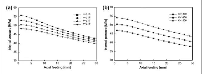
Kim et al. (Kim et al., 2006) investigated the influence of material parameters, n-value and strength coefficient (K-value), on bursting pressure. Their results showed that the bursting pressure increases by increasing the K-value or by decreasing the n-value as presented in Figure 1.4.

Figure 1.4: The effect of n-value and K-value on bursting pressure (Kim et al., 2006)

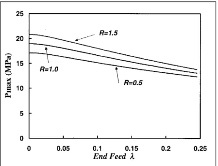
The other important material parameter in THF is anisotropy (r-value). Fuchizawa (Fuchizawa, 1987) explored the effect of r-value on deformation of thin-wall tubes in hydroforming process. His study showed the critical role of the r-value in THF process. Based on his results, anisotropy in longitudinal direction has considerable influence on expansion limit and thinning ratio while anisotropy in hoop direction affects the required internal pressure. Xia (Xia, 2001) studied the effect of r-value on bursting pressure through a mathematical analysis (Figure 1.5). He presented the results of his research as hydroforming failure diagram in the end feed—internal pressure space. Other researchers reached to the same results for the effect of r-value in THF process (Carleer et al., 2000; Kim et Kim, 2002; Manabe et Nishimura, 1983).

Figure 1.5: The effect of r-value on bursting pressure in THF process

1.1.2 Effect of geometrical factors

Geometrical factors have an important influence on the THF process. The effect of the tube diameter on formability and thickness variation in THF of a vehicle bumper rail with complex cross section was investigated by Kang et .al (Kang, Kim et Kang, 2005). They found that increasing the tube thickness by 10% will decrease the thinning rate by one-third and will result in more uniform thickness distribution. Also, for the tubes with outer diameter more than 100 mm the influence of the pre-pressure is more distinct. Koc et al (Koç et al., 2000) used Low Cost Response Surface Method (LCRSM) which is a design of experiments technique along with FE simulations to study the effect of geometrical parameters on T-shape THF process as plotted in Figure 1.6. With this study, they concluded that the most affecting parameters on bulge height (Hp) are the distances between protrusion and edges

(Lpe1 and Lpe2).

Figure 1.6: The effect geometrical parameters on bulge height in T-shape THF

Kridli et al. (Kridli et al., 2003) investigated the effect of the die corner radius and initial tube thickness on corner filling and thickness distribution in a square cross section THF process. They concluded that with a larger corner radius, more uniform thickness distribution is attainable. Also, they reported that the initial thickness mostly affects the required internal pressure and the thinning pattern remains the same for all the thicknesses. In another research, the effects of tube outer diameter on hydroforming with a square cross section die performed by Kömmelt (Kömmelt, 2004). He concluded that by increasing the tube diameter, the thickness distribution of the hydroformed part will be more uniform.

1.1.3 Effect of loading path

The effect of loading path (internal pressure and axial loading) during the THF process is a key factor for production of a sound hydroformed part. Therefore, considerable researches have been carried out by various researchers on this matter. In 1968, Ogura and Ueda (Ogura et Ueda, 1968) investigated the effect of internal pressure and axial loading in T-branch hydroforming of low and medium carbon steel tubes. A variety of combinations of internal pressure and end feed were tested and finally a proper forming zone was defined for the T-branch hydroforming. In 1973, Limb et al. (Limb et al., 1973) presented their results on bulge forming of different materials with different thicknesses. They found that applying internal pressure and axial feeding simultaneously leads to better thickness distribution and tube expansion. In the same year, Woo (Woo, 1973) studied the effect of internal pressure and axial-feeding in bulge forming of copper tubes experimentally and numerically. The stress-strain relationship in his FE simulation was obtained from bi-axial test and the results were in good agreement with experimental results. In 1976, a study was carried out by Kandil (Kandil, 1976) on THF of tubes with different materials such as Brass, Aluminum and Copper using only internal pressure. Manabe et al. (Manabe et al., 1984) used an analytical approach to predict the required internal pressure and axial load for hydroforming of aluminum tubes. Then a computer control press was used to implement predefined loading paths to investigate the deformation behavior and forming limits of the aluminum tubes. In a later research, two different loading paths: pressure predominant and feed predominant

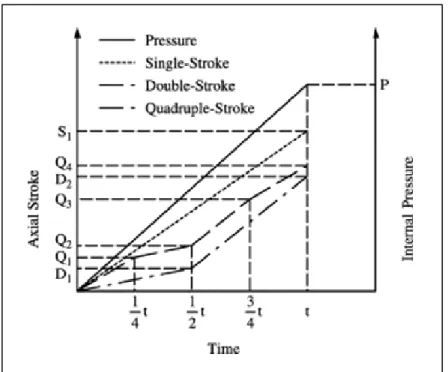
loading path were compared to each other by Ahmed and Hashmi (Ahmed et Hashmi, 1998). They concluded that using pressure predominant loading path leads to better deformation as feed predominant loading path may result in buckling or wrinkling. Ahmetoglu et al. (Ahmetoglu et al., 2000) in their study declared that it is better to increase the axial feed to obtain better wall thickness uniformity. However, by increasing the end feed the required internal pressure increased too. Effect of axial load on wall thickness distribution was studied by Manabe and Amino (Manabe et Amino, 2002) analytically and numerically. They observed that axial feeding and lubrication condition have a great influence on tube thickness distribution in THF process. Koc (Koç, 2003) studied the effects of loading path and material properties of blank tubes in hydroforming process of a production scale automotive structural frame part. The results showed the significant effect of loading path on the final part. The effect of three different end conditions: free end, fixed or pinched end and forced end on forming limit diagram (FLD) of aluminum alloy AA6082-T4 were examined by Imaninejad et al. (Imaninejad, Subhash et Loukus, 2004). It was noticed that free end condition has the lowest forming limit followed by fix end and forced end conditions. They also found that weld material anisotropy and end-condition are the two major parameters that affect the failure location in hydroforming of the tubes. In a subsequent work Imaninejad et al. (Imaninejad, Subhash et Loukus, 2005) suggested multiple strokes for axial and vertical actuators to improve the formability of the process (Figure 1.7). Also they found that the majority of the axial feed should be provided after tube material yielding under internal pressure.

Hama et al. (Hama et al., 2006) developed FE simulation to study the effect of three different loading paths: pressure advanced, linear and feed advanced (Figure 1.8) on THF process with a rectangular cross section die. The results showed that the pressure advanced loading path in which the internal pressure increases to a certain amount prior to starting the axial feeding leads to better formability as the initial internal pressure prevents the local wrinkling in the early stage of the process and thus the compressive longitudinal stress will be attained in the whole process.

Figure 1.7: Schematic of single and multiple strokes axial feed paths in THF (Imaninejad, Subhash et Loukus, 2005)

Figure 1.8: (A) Pressure advanced, (B) Linear, and (C) Feed advanced loading paths

However, in another study performed by Ray (Ray et Mac Donald, 2005) on X-shape tube hydroforming, it was recommended to use feed advanced loading path as pressure advanced loading path may causes bursting due to excessive wall thinning at certain weak points or sensitive zones. Kang et al. (Kang et al., 2007) conducted hydroforming experiments with different die shapes such as rectangular, circular and triangular for production of metallic elbows. It was concluded that proper axial feed avoids occurrence of cracks in all the cases. In a later study by Varma et al. (Varma et Narasimhan, 2008), the effects of two different pressurizing methods: prescribing fluid pressure and specified volume flow rate were investigated. They found that using specified volume flow rate method leads to proportional strain path while using prescribing fluid pressure will results in non-proportional strain path.

1.1.4 Effect of friction and lubrication

High contact pressures and large contact surfaces between the die and the tube in THF process lead to high frictional forces between the tube and the die. Furthermore, as mentioned before, in most cases in the THF process, axial feeding is required to feed the material into the deforming zone. In addition, hydroforming from a circular cross section to the die cross section requires minimum material movement resistance to fill the die completely. Therefore, careful consideration should be taken to decrease the friction between the tube and the die to avoid failures such as bad surface quality due to sticking and galling or bursting due to excessive thinning. Schmoeckel et al. (Schmoeckel et al., 1997) classified three different friction zones: guiding zone, transition zone and expansion zone in a typical THF process as presented in Figure 1.9. Base on their study, the friction condition, sliding velocity and stress state identified to be different in each of the mentioned zones. In the guiding zone, compressive state of the stress, high sliding velocity and low surface strains are governing. In the transition zone the expansion or reduction of the tube is notable. The stress state consisted of compressive stresses due to the axial load and tensile hoop stresses due to expansion of the tube and the sliding velocity is less than the guiding zone, but still appreciable. In the expansion zone, sliding velocity is negligible and tube expansion is large and tensile stresses in hoop direction are dominant.

Figure 1.9: Friction zones in THF (Plancak, Vollertsen et Woitschig, 2005)

The parameters that affect the friction condition are categorised to four groups: (I) process parameters, such as internal pressure, (II) tool parameters like die surface finish and die hardness, (III) workpiece parameters, such as tube surface condition and tube material properties and (IV) lubricant (Ahmetoglu et Altan, 2000).

Lubrication in THF process is very important; as a good lubrication allows the tube to expand much more than a bad lubrication, which causes excessive friction stress and will result in wrinkling, bursting or bad surface quality. To evaluate lubricants for hydroforming applications, different tests have been proposed (Koç, 2008). Corner fill test and Pear-shaped expansion test are two main experimental methods to evaluate the lubricants for hydroforming applications. In the corner fill test (Figure 1.10a), the tube corner radius along with wall thickness distribution are two references for evaluating the lubricant performance. In pear-shaped expansion test (Figure 1.10b), the performance evaluation of the lubricants can be achieved based on wall thinning distribution, protrusion height (δ) and bursting pressure.

Figure 1.10: (a) Corner fill and (b) Pear-shaped expansion test for evaluate the lubricants in expansion zone

(Koç, 2008)

Studying the effects of friction and lubrication in THF process date back to 1973 when Limb et al. (Limb et al., 1973) presented their results on the effect of friction and different lubrications on protrusion height in T-branch hydroforming process. It was reported that a lower protrusion height was obtained and the bulged dome of the T branch became more pronounced due to improper lubrication condition while proper lubrication condition resulted in higher protrusion height as well as a flat bulge protrusion area. Lee et al. (Lee, Keum et Wagoner, 2002) designed a sheet metal friction tester to investigate the effect of lubricant viscosity on friction. The results showed that the lubricant viscosity has an inverse relation with coefficient of friction (COF). In the same paper the effect of surface roughness on COF was investigated. They concluded that for all lubricants in an extremely high (< 1 μm) or low (> 0.5 μm) surface roughness, the COF is higher. The COF in guiding zone for different materials and different lubricants was studied by Vollertsen and Plancak (Vollertsen et Plancak, 2002) using an experimental procedure that is called upsetting test. Tube upsetting test was recognised a good mean for evaluating COF for the processes with plastic deformation. Ngaile et al. (Ngaile, Jaeger et Altan, 2004a; 2004b) studied lubrication mechanisms and the appropriate tests for measuring the COF in transition and expansion zones. They concluded that the limiting dome height (LDH) and pear-shaped expansion tests are appropriate for evaluating the COF in transition and expansion zones, respectively. Yeong-Maw et al. (Yeong-Maw et Li-Shan, 2005) investigated the effect of axial feeding

velocity and internal pressure on COF. They found that by increasing the internal pressure, the contact surface increases resulting in the tube surface roughness decreases, which leads to a decrease in the COF. Also, they found that axial feeding velocity has not significant effect on COF value. Plancak et al. (Plancak, Vollertsen et Woitschig, 2005) proposed an analytical model based on the tube-material properties and the tube geometry before and after deformation in the tube-upsetting test for calculating the COF. They also concluded that higher amount of internal pressure will results in lower COF values and by decreasing the friction, the thickness variation decreases too. An analytical model was proposed by Orban and Hu (Orban et Hu, 2007) to study the effect of the COF and material properties on wall thickness distribution in THF process. They explained how a sticking friction develops and restricts the material from further stretching. In a recent study, Yi et al. (Yi et al., 2011) investigated the COF in three different die shapes. They found that an increase in lubricants viscosity, tube diameter and tube material strength, the COF decreases. It was reported that the COF in guiding zone is lower than that in expansion zone and the die shape does not have any effect on the COF.

1.2 Instabilities and failures

THF is a highly nonlinear process in which loads in different directions and ratio acts during forming process. So, it is important to delimit affecting parameters to avoid instability and defects throughout the process. The loading limits in the THF process are imposed by three main failure modes namely: buckling, wrinkling and bursting (Figure 1.11). The danger of buckling prevails especially at the initial stages of hydroforming process when excessively high axial load is applied on long tubes. Wrinkling is most probable at initial and intermediate stages of hydroforming. Depending the severity of the wrinkle, it may be eliminated by increasing the internal pressure. During the final stage of the forming process, high internal pressure along with insufficient material flow may cause local necking and finally bursting of the tube. These failure modes can be postponed or avoided through the adjustment of tube material properties, friction condition, process control parameters and tool design.

Figure 1.11: Different failure mode in THF process (Abrantes, Szabo-Ponce et Batalha, 2005)

In order to achieve a defect free workpiece in THF process, a proper load path should be considered. A proper load path for a THF process resides within the operating window (Figure 1.12) which varies for different material and different tube dimensions.

Figure 1.12: Process windows for THF process (Kim et Kim, 2002)

Bursting as one of the failure modes in THF process is an irrecoverable defect in contrast with buckling and wrinkling. Therefore, predicting the bursting is from a high degree of

importance. Failure limit diagram (FLD) is a standard approach for measuring the formability in sheet metal forming and burst prediction. For generating the FLD, a series of material failure tests have to be done. By plotting major strain versus minor strain for different linear strain paths, the FLD can be generated. The formability limit on a FLD is presented as a line at which failure is onset and is called failure limit curve (FLC). The area below the FLC shows the safe region while the area above the FLC represents the failed region. Figure 1.13 shows a typical FLD and different linear strain paths.

Figure 1.13: A typical FLD

(Holmberg, Enquist et Thilderkvist, 2004)

Koc and Altan (Koç et Altan, 2002) developed an analytical model based on membrane and thin-thick walled tube theories to predict the process limits and parameters in THF process. Although their model was not designed for complex parts, it could give an initial guess for further investigation with the use of FEA. An analytical model for analysing the tube material properties effect on different failure mode was determined by Chu et al. (Chu et Xu, 2004). Their study showed that the geometrical parameters such as the ratio between the initial tube thickness to the initial tube radius (t0/r0), the ratio between the initial tube radius

to the initial tube length (r0/l0) and work hardening coefficient have great effect on the

dominant failure in short tubes while buckling occurs in longer tubes. In a different investigation, the bursting of seamed tube in bulge tube hydroforming was studied by Kim et al. (Kim et al., 2004) through FEA. They found that the initial fracture takes place on heat affected zone near the weld line. Yuan et al. (Yuan et al., 2007; Yuan, Yuan et Wang, 2006) divided the wrinkling effect in THF into three groups including dead wrinkles, that are not removed by the end of THF, bursting wrinkles, that result to bursting of the tube and useful wrinkles, that can be removed by the end of THF. They mentioned that while the dead and bursting wrinkles considered as defects, useful wrinkles can improves the expansion ratio in THF. But the drawback of useful wrinkles is the ununiform thickness distribution along the axial direction. The minimum wall thickness is found at top of wrinkle wave whereas the maximum wall thickness can be found in the bottom of wrinkle wave.

1.3 Finite element modeling

As discussed before, THF has many advantages, though it is quite a complex process due to many parameters involve in it, such as formability of the material, loading path (end feeding force and internal pressure), tool geometry and friction. Hence having a good understanding of these parameters helps to improve the quality of the final part. Hydroforming try-outs to investigate the effect of these parameters is expensive and highly time consuming. Therefore, the application of numerical simulation for investigating and optimizing the hydroforming process has become a standard practice for engineers. The FEA can be used at designing stage to verify the feasibility of the process and to predict failure location. In this stage the FEA helps to improve the part design. In the next stage, the computer simulation along with optimization algorithms can be used to optimize the process parameters.

The history of using FEA for metal forming processes dated back to 1960s when the first commercial FEA codes were developed. At that stage due to the technological limitations, the application of the FEA was restricted to deformations with less than 1% strain. By the end of 1970s, a few nonlinear FE solvers was introduced to the world. But only by the beginning of 1990s the use of FEA became a standard tool for researchers to investigate the

metal forming processes (Alaswad, Benyounis et Olabi, 2012; Koç et Altan, 2001). Nowadays, many commercial FE modeling softwares such as LS-DYNA, ABAQUS, ANSYS, AUTOFORM are used to predict the output of the metal forming processes.

Depending on the complexity of the analysis and the required degree of accuracy, the FE model can be constructed with a wide range of options; from a simple implicit two-dimensional (2D) model to a very complex explicit three-two-dimensional (3D) model. Because of the severe non linearity due to large deformations, plastic behavior of the material and contact conditions in THF process, usually a 3D model is required to present the real forming condition and make it possible to detect forming defects during the process, such as wrinkling and buckling. From the formulation point of view, there are two types of approaches to develop FEM; implicit and explicit formulations. The implicit approach is mainly used for analyzing the static models while the explicit approach is used for dynamic ones. There are also a few processes that can be analysed either by implicit or explicit formulation. These processes are called quasi-static problems. THF can be considered as a quasi-static problem due to the low strain rates during the process. Modeling the THF process with either of the formulations has its own pros and cons. An implicit formulation is less time consuming and is effective especially for simplified problems. Many researchers have used this technique to reduce the processing time (Ahmed et Hashmi, 1998; Koç et al., 2000; Mac Donald et Hashmi, 2000; Ray, 2005). But implicit approach is not as effective as explicit technique when dealing with more complex problems. Explicit formulation has better capabilities for modeling nonlinear problems with high degree of deformations and gives a better insight into the forming process (Rebelo et al., 1992). There are many parameters to take in consideration for developing an accurate and efficient FE model; assumptions and simplifications, elements type, mesh density, boundary conditions and material formulation.

In 1991, Lange et al. (Lange et al., 1991) developed a finite element code for modeling metal forming processes like bending and bulge forming base on elasto-plastic material model. Ahmed and Hashmi (Ahmed et Hashmi, 2001) used LS-DYNA software to simulate the

T-branch bulge forming under two different loading conditions. Because of the symmetry, only a quarter of the problem was modeled using solid elements to describe both the die and the tube. A piecewise linear plastic material model was used to describe the tube while the die was considered as rigid. They showed that with the same axial load rate, using the lower internal pressure rate will results in more uniform stress strain distribution and will enable the internal pressure to reach to the higher values. The comparison between implicit and explicit method in FEA for predicting the wrinkling in THF process was investigated by Kim et al. (Jeong, Sung-Jong et Beom-Soo, 2003). They also studied the effects of time scaling and mass scaling in explicit method. It was explained that implicit method requires more attention especially for friction force calculation while the dynamic explicit method leads to more reasonable results that are in good agreement with experimental results. Also they concluded that for a suitable scaling factor, the kinetic energy must be less than 0.1 of the internal strain energy. The effect of internal pressure in THF process was investigated using FE simulations by Nikhare et al. (Nikhare, Weiss et Hodgson, 2009). The results showed that in high pressure tube hydroforming (HPTH) the stress variation and thinning are more pronounced that low pressure tube hydroforming (LPTH). Also it was showed that HPTH is more sensitive to friction than LPTH.

1.4 Process optimization

Finding the optimum combination of the process parameters in THF in order to produce the desired part have been always the main challenge for manufacturer. The traditional method of trial and error is time consuming and non-systematic and usually does not lead to optimum combination of input parameters. Though, optimization methods along with FE simulations can help to overcome this problem. These methods can be classified in two major groups: adaptive simulation methods and optimisation procedures (Jansson, Nilsson et Simonsson, 2007).

In the adaptive method, the FE simulation is continuously monitored for defects and input parameters are adjusted in each subsequent time increment. This procedure was used by

many researchers to optimise the loading path in THF process (Aydemir et al., 2005; Johnson et al., 2004; Labergere et Gelin, 2004; Ray et Mac Donald, 2004; Sillekens et Werkhoven, 2001a). The advantage of this method is the optimum parameters can be obtained in only one FE simulation.

The optimisation procedures try to find the optimum solution in an iterative way and by using the constraints of the process. The optimisation methods divided in three sub groups including (I) iterative algorithms, (II) evolutionary and genetic algorithms (GA) and (III) approximate optimization algorithms (Meinders et al., 2008). Classical iterative optimisation algorithms like conjugate gradient, BFGS, etc try to find the optimum solution based on minimisation of an objective function and with repeating FE simulations. As illustrated in Figure 1.14a, there is a direct interface between the FE simulation and optimisation algorithm in iterative optimisation methods which means for each function evaluation of the algorithm a FE calculation needs to be run. Despite these algorithms are well known and widely spread which is their advantages, they may trap in local optimum solutions instead of the global ones which is disadvantageous of these techniques. However, these methods have been used by many researchers to optimise the THF input parameters. (Endelt et Nielsen, 2001; Fann et Hsiao, 2003; Jirathearanat et Altan, 2004; Sillekens et Werkhoven, 2001b; Yang, Jeon et Oh, 2001).

To overcome the disadvantages of iterative algorithms, GA can be used to find the global optimum solution. The GA is an optimising method that mimics the process of natural evolution. However, the large number of required FE simulations in this method makes it very time consuming and is considered as a serious drawback. Abedrabbo et al. (Abedrabbo et al., 2011) used this method and LS-DYNA finite element code to optimise the load path in THF process.

Figure 1.14: (a) Direct and (b) approximate optimisation

(Meinders et al., 2008)

The last group of optimisation method is the approximate optimization algorithms. Response surface methodology (RSM) is a well known method among this group. In this method a set of input parameters are chosen and through FE simulations, the response to each of these sets are calculated. Then a low order polynomial is used to fit through response points and the best combinations are used for the next step, by repeating this process the optimized combination could be found. In this approach there is not a direct link between FE simulation and optimization algorithm as it was in two previous methods and a metamodel is placed in between as a buffer (Figure 1.14b). Kriging and neural networks are two other metamodeling techniques. Compared to iterative algorithms, approximate optimization algorithms have the ability to find the global optimum solution and at the same time they are less time consuming compared to evolutionary algorithms. These advantages make it appealing for researchers in metal forming process (Alaswad, Olabi et Benyounis, 2010; 2011; Koç et al., 2000).

CHAPTER 2

Methodology

THF is an advanced metal forming process that requires special attention in designing the part/tool and developing the process parameters due to hard tooling involved in it. The process development stage is an expensive and time consuming part of the THF process in complex shapes. Thus, using a trial and error procedure for developing a THF process is not an option and using FEA as a predictive tool seems inevitable. FEA increases the efficiency by reducing the lead time and the total cost of manufacturing through eliminating the trial and error procedure. To conduct FEA, a FEM with appropriate geometrical contacts, boundary conditions and material model has to be developed. Once the results of the FEA are verified by the experimental results it can be used to study the affecting parameters and to predict the failure/defects and critical regions in the THF process of components with similar complexity.

The first goal of the present work is to study the effects of different process parameters such as geometrical characteristics, load path and friction condition in the THF process. Therefore, a FEM, that will be described, was developed and validated by comparing the numerical and experimental results.

2.1 Finite element model (FEM)

The FEM that was used in this study consisted of two parts; (i) tube and (ii) rigid die. The process is called round-to-square hydroforming as it starts with a tubular shape material and the final product has a square shape. Due to symmetry planes over the tube length and the cross section, the model was simplified by applying the symmetry boundary conditions to the boundary nodes along the symmetry planes. Only half of the length and one quarter of the cross section of the tube and the die were used in the simulation (Figure 2.1). The initial tube

length and the outer diameter were 220 mm and 50.8 mm (2”) respectively. The tube material was stainless steel 321 (SS321) with two different wall thicknesses; 0.9 mm and 1.2 mm.

Figure 2.1: Symmetry planes

The tube thickness was varied in the circumferential direction for both tube thicknesses, so the average values of the thicknesses (0.94 mm and 1.22 mm) were used for modeling the tubes. Ansys v13.0 was used to mesh the model and Ls-Dyna v970 was used as the FEM solver. 4619 four nodes Belytschko-Tsay shell elements with aspect ratio of 1 and with five integration points through the thickness were used to generate the tube model. As shell elements are not able to capture the through thickness stress, two other models were generated using solid elements and thick-shell (Tshell) elements to compare the results. Tshell element is a special element in LS-DYNA which is developed to have both advantages of solid and shell elements. It can capture 3D stresses like solid element, but it needs less computation time. The solid model was generated using 13279 constant stress solid elements with three elements through wall thickness. The aspect ratio of the solid elements for the FEM of both tubes thicknesses was equal to one. The Tshell model consisted of 8839 elements with 2 elements through thickness, as recommended by LS-DYNA (LS-Dyna

Keyword User's Manual, 2013). The aspect ratio of the TShell elements for the FEM of both tube thicknesses was equal to one. The die was modeled as rigid body using 6669 four nodes shell elements. Figure 2.2 illustrates the FEMs with different element types.

Figure 2.2: (a) shell and (b) solid FEM

2.1.1 Contact condition

To simulate the contact condition between the tube and the die, a surface to surface contact (CONTACT_SURFACE_TO_SURFACE) with Coulomb friction law was applied and different COF values from 0.01 to 0.2 were applied to study the effect of COF on thickness variation and the expansion of the tube. In the shell element model, to avoid tube self

penetration in case of wrinkling or buckling, a contact with single surface entity (CONTACT_AUTOMATIC_GENERAL) was defined for the tube.

2.1.2 Load path simulation

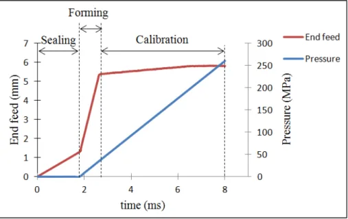
For simulating the load path during the process, different displacement curves were assigned to the tube end nodes to simulate the end feed condition. A linear path was defined for increasing the internal pressure during the process. As shown in Figure 2.3, the forming process consisted of three stages: (a) sealing, (b) forming and (c) calibration stages. At the beginning of the process a displacement was applied to the end of the tube to mimic the sealing operation. During the experiments it was noticed that in order to seal the tube end we need 35 kN load which was obtained at 1.2 mm end feed displacement. During the sealing period the internal pressure is equal to zero. At the second stage of the process, while the internal pressure starts to increase linearly, the end feed increases with a high slope. In the last part of the process or the calibration stage the internal pressure continues to increase while there is no noticeable end feeding. This load path was obtained from the experiment, which will be described later in the THF experiments section.

2.1.3 Material model

In order to simulate the tube material behavior, the Swift work hardening law (Equation 2.1) was used.

σ = K(ε0+ε)

where σ is the true stress, ε0 is the initial true strain, ε is the true strain, K is the strength

coefficient and n is the strain hardening exponent. The material properties were used from an ongoing study in the THF process. The material was considered isotropic and the material properties of the tubes (0.9 mm and 1.2 mm) were extracted by performing free expansion test and tensile test. The samples for tensile test were cut from the tubes based on ASTM E8. Using the data obtained from the free expansion test and tensile test the values for ε0, K and n

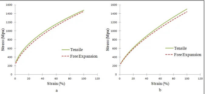
were obtained. Table 2.1 summarizes the experimental material parameters used for the SS321 tubes. Figure 2.4 illustrates the related true stress-strain curves for both tube thicknesses, which are extrapolated up to 100% strain.

Table 2.1: Material properties of the SS321 tubes Stainless Steel (SS321)

Material

Thickness = 0.9 mm Thickness = 1.2 mm Free Expansion Tensile Free Expansion Tensile

K (MPa) 1427.4 1458.29 1397.8 1461.54

n 0.53 0.49 0.62 0.62

ε0 0.03 0.026 0.05 0.048

Yielding Stress (MPa) 250 260

Density (g/mm³) 8.0E‐03 8.0E‐03

Elastic Modulus (MPa) 193.00E+03 193.00E+03

Figure 2.4: True stress-strain curves for tubes with (a) 0.9 mm and (b) 1.2 mm thicknesses

2.1.4 Time scaling

According to Jeong et al. (Jeong, Sung-Jong et Beom-Soo, 2003) for time scaling in quasi static processes like hydroforming, the kinetic energy should be maintained less than 10% of the internal strain energy during the simulation. In this case the dynamic effect in explicit method, which may affect the results accuracy in FEA, will be minimized. Therefore, different simulation durations were tested and their ratio of the kinetic energy to the internal strain energy was checked to find an appropriate time scaling for the simulations. After a few trials, 8 ms was selected as termination time. In other words, to minimize the dynamic effect in the simulation and to avoid high computational costs, the total hydroforming process was modeled in 8 ms compared to 150 s in the experiments. The hydroforming codes for shell, solid and Tshell FEMs are shown in Appendix A.

2.1.5 Spring back

After the hydroforming simulation, a file was generated (Dynain file) by LS-DYNA which contained the deformed mesh, stress, and strain state of the tube. This file was used as an

input for the spring back simulation, using a static implicit solver in LS-DYNA. The material information used in the spring back simulation was the same as the hydroforming simulation. The spring back code is presented in Appendix B.

2.2 Experimental setup

In order to verify the FEA results, the experimental data is required. The THF experiments were conducted at NRC using a fully equipped hydroforming press manufactured by Interlaken Technology Corporation (Figure 2.5).

Figure 2.5: Hydroforming press at NRC

The vertical cylinders of the press delivers a 1000 ton clamping force and the two horizontal cylinders provide maximum capacity of 1000 kN axial load at each end of the tube. The

pressure intensifier unit of the press was designed to apply a maximum internal pressure of 413 MPa (60000 Psi). To perform the THF experiments, a tooling system consisted of the die, end plungers and expansion measurement units was designed and manufactured at NRC.

2.2.1 Die

A round-to-square die set was designed and manufactured at NRC. The die was made of hardened tool steel and had a square cross section with corner radii of 2.4 mm. In Figure 2.6, the die and its guiding zone, transition zone and expansion zone are illustrated.

2.2.2 Plungers

The plungers (Figure 2.7) were designed and mounted on the left and right horizontal cylinders of the press. The plungers slide in the guiding zone of the die and apply the axial load on both ends of the tube. The sealing shoulder of the plungers provides the sealing required during the hydroforming process.

Figure 2.7: Plungers setup

2.2.3 Expansion measurement unit

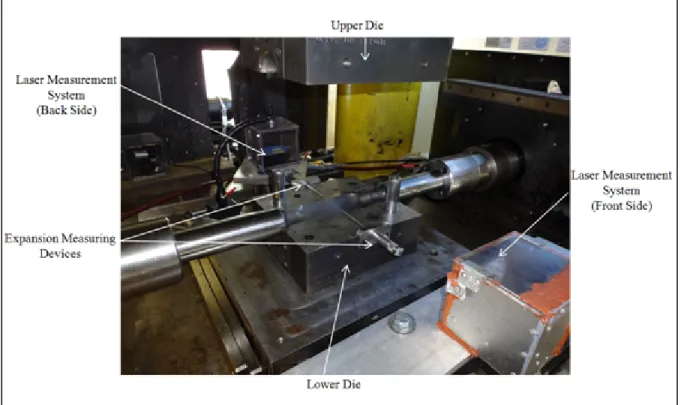
The distance that the tube expands at the corners of the square was considered as the expansion of the tube (Figure 2.8). To monitor the expansion of the tubes during the THF process, two laser measurement systems in conjunction with two expansion measurement devices, implemented inside the die, were used during the experiments. As illustrated in Figure 2.8a, at the beginning of the process the distance between the laser measurement unit

and the expansion measurement device is equal to L0. As the hydroforming process starts, the

tube pushes the pins outward and as the result, the value that is read by laser measurement unit at each time increment (Ln) decreases (Figure 2.8b). The laser measurement units were

connected to the data acquisition system of the press and record the expansion of the tube during the THF process. The difference between the Ln and L0 was considered as the

expansion of the tube at each time increment. In Figure 2.9 the expansion measurement unit setup on the hydroforming press is presented.

Figure 2.9: Setup of the expansion measurement units

2.2.4 Tube preparation

Before the THF experiments, the tubes were cut with a band saw and the two ends of the tube were straight cut, using a turning machine, to the final length of 220 mm. Then, the outer surface of the tube was polished by a sandpaper (CAMI Grit designation = 100) to prepare the surface for electrochemical etching. To check the thickness uniformity in the blank tubes, the thicknesses were measured in longitudinal and circumferential directions using an ultrasonic thickness measurement device (38DL Plus) manufactured by Olympus Corporation company (Figure 2.10).

It was noticed that the thickness along longitudinal direction was uniform while in circumferential direction the thickness variation was about 0.05 mm and 0.07 mm for the 0.9 mm and 1.2 mm thick tubes, respectively (Figure 2.11).

Figure 2.10: The ultrasonic thickness measurement device (38DL Plus)

Figure 2.11: Circumferential thickness variation for tubes with (a) 0.9 mm (b) 1.2 mm thickness (dimensions in mm)

In order to be able to measure the strains after the hydroforming process, a pattern of black circle dots was etched on the outer surface of the tubes. Since the tubes are in contact with

the die during the hydroforming process, electrochemical etching process was required to get more stable dots on the tubes, so the dots will be more visible at the contact zone between the tube and the die after deformation. The electrochemical etching system consisted of an anode (positive pole), a cathode (negative pole), power unit, electrolyte solution and a stencil sheet. The stencil is used to produce the dot pattern on the surface of the tube. In our case, the dot pattern was 1mm in diameter with 2 mm distance between the centers of the dots (Figure 2.12).

Figure 2.12: Pattern produced on the tube surface

In order to investigate the effect of lubrication in the THF process, two different lubricants were applied on the surface of the tubes using an air spray device. To obtain the best lubrication condition, the lubricant thickness should be between 0.04 to 0.06 mm according to the manufacturer. After the lubricants dried, the thickness of the lubricants on the surface of the tubes was measured for uniformity, using an ultrasound device to check that a uniform lubrication was applied on the surface of the tubes.

2.2.5 Hydroforming

After the tube preparation, the tubes were placed inside the die for the hydroforming process. As mentioned before, the pressure intensifier of the press was capable of delivering 413 MPa (60000psi) internal pressure, but during the experiments it was noticed that 260 MPa pressure is enough to fill the die completely in all cases. For this reason 260 MPa was selected as the maximum internal pressure for the experiments. During the experiments, the pressure started from zero at the end of the sealing stage at the beginning of the forming stage and increased linearly up to the maximum value of 260 MPa.

The control system of the press has the ability to end feed material into the die cavity in two different methods: (i) force control and (ii) position control. In the first method, the amount of axial load at the tube ends is specified while in the second method the position of the plungers during the hydroforming process is controlled by the control system of the press. A typical THF process is divided into three stages including sealing, forming and calibration stages (Figure 2.13). At the beginning of the experiments (sealing stage), a 35 kN sealing force was applied at tube ends, using the force control method. For the forming and calibration stages two different approaches were used. In the first approach, the force control method was used in the forming and calibration stages to conduct a free end hydroforming process. During the free end hydroforming, the end feeding forces that are applied to the tube are enough to only hold the sealing during the process and no material is fed into the die cavity. To calculate the required end feeding force at any specific time, the following equation was used:

F = P.A/1000+35

Where F is the end feeding force in kN, P is the internal pressure in MPa at any given time and A is the plunger’s cross section area in mm2_{. 35 kN in this equation is the initial sealing}

force before applying the internal pressure. According to the equation 2.2, by increasing the internal pressure the end feeding force increases, compensating the opposing force on the