Monitoring for Disruptions in Financial Markets

Texte intégral

(1)2004s-26. Monitoring for Disruptions in Financial Markets Elena Andreou, Eric Ghysels. Série Scientifique Scientific Series. Montréal Mai 2004. © 2004 Elena Andreou, Eric Ghysels. Tous droits réservés. All rights reserved. Reproduction partielle permise avec citation du document source, incluant la notice ©. Short sections may be quoted without explicit permission, if full credit, including © notice, is given to the source..

(2) CIRANO Le CIRANO est un organisme sans but lucratif constitué en vertu de la Loi des compagnies du Québec. Le financement de son infrastructure et de ses activités de recherche provient des cotisations de ses organisations-membres, d’une subvention d’infrastructure du ministère de la Recherche, de la Science et de la Technologie, de même que des subventions et mandats obtenus par ses équipes de recherche. CIRANO is a private non-profit organization incorporated under the Québec Companies Act. Its infrastructure and research activities are funded through fees paid by member organizations, an infrastructure grant from the Ministère de la Recherche, de la Science et de la Technologie, and grants and research mandates obtained by its research teams. Les organisations-partenaires / The Partner Organizations PARTENAIRE MAJEUR . Ministère du développement économique et régional et de la recherche [MDERR] PARTENAIRES . Alcan inc. . Axa Canada . Banque du Canada . Banque Laurentienne du Canada . Banque Nationale du Canada . Banque Royale du Canada . Bell Canada . BMO Groupe Financier . Bombardier . Bourse de Montréal . Caisse de dépôt et placement du Québec . Développement des ressources humaines Canada [DRHC] . Fédération des caisses Desjardins du Québec . GazMétro . Hydro-Québec . Industrie Canada . Ministère des Finances du Québec . Pratt & Whitney Canada Inc. . Raymond Chabot Grant Thornton . Ville de Montréal . École Polytechnique de Montréal . HEC Montréal . Université Concordia . Université de Montréal . Université du Québec à Montréal . Université Laval . Université McGill . Université de Sherbrooke ASSOCIE A : . Institut de Finance Mathématique de Montréal (IFM2) . Laboratoires universitaires Bell Canada . Réseau de calcul et de modélisation mathématique [RCM2] . Réseau de centres d’excellence MITACS (Les mathématiques des technologies de l’information et des systèmes complexes) Les cahiers de la série scientifique (CS) visent à rendre accessibles des résultats de recherche effectuée au CIRANO afin de susciter échanges et commentaires. Ces cahiers sont écrits dans le style des publications scientifiques. Les idées et les opinions émises sont sous l’unique responsabilité des auteurs et ne représentent pas nécessairement les positions du CIRANO ou de ses partenaires. This paper presents research carried out at CIRANO and aims at encouraging discussion and comment. The observations and viewpoints expressed are the sole responsibility of the authors. They do not necessarily represent positions of CIRANO or its partners.. ISSN 1198-8177.

(3) Monitoring for Disruptions in Financial Markets * Elena Andreou†, Eric Ghysels‡. Résumé / Abstract Nous étudions les tests CUSUM historiques et séquentiels pour des séries dépendantes avec des applications en finance. Pour les processus temporels, une nouvelle dimension se présente : l’effet du choix de la fréquence des observations. Un nouveau test est également proposé. Ce test est basé sur une formule de prévision locale d’un pont brownien. Mots clés : changement structurel, CUSUM, GARCH, variation quadratique, ‘power variation’, données de haute fréquence, pont Brownien, puissance locale, tests séquentiels.. Historical and sequential CUSUM change-point tests for strongly dependent nonlinear processes are studied. These tests are used to monitor the conditional variance of asset returns and to provide early information regarding instabilities or disruptions in financial risk. Data-driven monitoring schemes are investigated. Since the processes are strongly dependent several novel issues require special attention. One such issue is the sampling frequency. We study the power of detection as sampling frequencies vary. Analytical local power results are obtained for historical CUSUM tests and simulation evidence is presented for sequential tests. Finally, a prediction-based statistic is introduced that reduces the detection delay considerably. The prediction based formula is based on a local Brownian bridge approximation argument and provides an assessment of the likelihood of changepoints. Keywords: structural change, CUSUM, GARCH, quadratic variation, power variation, high frequency data, Brownian bridge, boundary crossing, sequential tests, local power.. * We would like to thank the participants of the UCSD Conference in honor of Clive Granger and seminar participants at Tilburg University for comments. We also like to thank Valentina Corradi, Piotr Kokoszka, Theo Nijman, Werner Ploberger and BasWerker for insightful comments on various aspects of our work. The first author would like to acknowledge the financial support of a Marie Curie Individual Fellowship (MCFI-200101645). † Department of Economics, University of Cyprus. ‡ Department of Economics, University of North Carolina and CIRANO, Gardner Hall CB 3305, Chapel Hill, NC 27599-3305, phone: (919) 966-5325, e-mail: eghysels@unc.edu..

(4) 1. Introduction. One of Clive Granger’s very first papers was on the prediction of extreme events, namely floods of tidal rivers (see Granger (1959)). Since Granger’s early work there has been an enormous growth in the area of modelling extreme events in economics and finance (see e.g. Embrechts et al. (1997)). Despite the significant progress we made, there are still many outstanding issues. This paper is about monitoring for instabilities or disruptions in financial markets and the use of sequential testing procedures.1 Structural breaks and extreme tail observations are two types of rare events. The latter has been the main focus of risk management whereas the former represents a fundamental shift in the distribution of risky outcomes. Testing for breaks has obviously also close connections with model specification analysis as well as forecasting. Out-of-sample prediction is typically based on the maintained assumption of model (parameter) stability (see e.g. Hendry (1997)). Sequential analysis is therefore a desirable tool when out-of-sample analysis is performed since it allows for real-time monitoring of prediction models. Moreover, monitoring financial risk can be considered as a useful statistical tool for financial crises. So far, most statistical and econometric methods of sequential changepoint analysis have focused on linear regression models or linear dynamic models with weak dependence. Examples include Lai (1995, 2001), Chu et al. (1996), Leisch et al. (2000), Zeileis et al. (2004), among others. Notable exceptions are Altissimo and Corradi (2003) and Berkes et al. (2004) that will be discussed shortly. In this paper we are interested in monitoring stability of nonlinear strongly dependent processes. The interest stems from the fact that a large area of important sequential analysis applications is financial risk management. The daily reporting of some risk exposure measure has been adopted by many financial regulators. Embedded in most measures is a prediction rule based on a model for portfolio returns. For example, Value-at-Risk (VaR) attempts to forecast likely future losses using quantiles of the (conditional) portfolio return distribution and Expected Shortfall (ES) measures the expected loss given it exceeds some threshold. Andreou and Ghysels (2003) showed that ignoring structural change will lead to financial losses beyond those that can be anticipated by the routine application of 1 We will use the terms change-point and disruptions interchangeably. Hence, disruptions in financial markets are structural breaks, or change-points in the asset returns process.. 1.

(5) risk management estimation or simulation methods. The idea to monitor sequentially asset return related processes for change-points is still relatively unexplored and raises many issues. We focus exclusively on CUSUM-type tests and provide a number of contributions towards a better understanding of sequential testing for structural breaks in financial asset return processes or more generally nonlinear dynamic strongly dependent processes. In this respect our paper fits in a broader research program addressing the challenges of quality control for dependent monitoring processes (see e.g. Lai (2001, p. 317-8) and Stoumbos et al. (2000, p.994-5, sections 6 and 8)). The first issue we emphasize is the use of data-driven monitoring processes. Most of the literature so far has emphasized sequential testing via monitoring (individual) coefficients of parametric models. One of the main innovations in Andreou and Ghysels (2003) is the use of empirical monitoring processes that are purely data-driven and based on high frequency financial time series processes. Indeed, one virtue of financial market applications is the availability of high frequency price data for actively traded assets that bear neither sampling costs nor measurement error. These easy to collect and compute processes are practically appealing as even for the simplest representative parametric model for asset returns, e.g. a GARCH process, the likelihood function may be extremely complicated (for cases other than the Normal or Student’s t distribution) and therefore make parametric sequential analysis computational intensive and cumbersome. We do not necessarily advocate the exclusive use of data-driven tests, as parametric model-based tests can provide complementary information. For instance, Berkes et al. (2004) derive a sequential test for the parameters of a GARCH sequence. Their test could be used alongside the procedures presented here since they can provide information regarding the type of the change-point (e.g. constant versus dynamics of volatility). On the other hand Altissimo and Corradi (2003) deal with sequential tests for multiple breaks in the mean instead of the volatility of α-mixing processes.2 The second issue we explore is the effect of sampling frequency on the local power of CUSUM tests. Since we treat dependent processes, the choice of sampling frequency can be critical, an issue that has not been addressed in the literature since most of the emphasis has been on monitoring i.i.d. processes. Sampling frequency is indeed often one of the choice variables in the context of financial time series applications. We tackle the local asymptotic power 2. Andreou and Ghysels (2002) also consider multiple change-point tests in volatility.. 2.

(6) analytically in the context of a historical or off-line CUSUM statistic. More specifically, we find that the local power of the CUSUM-type ARCH tests for stability are inextricably linked with the sampling frequency choice and temporal aggregation involved in volatility models. This yields some interesting power trade-offs between the persistence and kurtosis properties of the process for different sampling frequencies. We focus exclusively on the ARCH(1) process where persistence and kurtosis are described each by a single parameter and quantify the trade-off between tail behavior, persistence, local power and sampling frequency. However, the analytical complexity of sequential CUSUM testing precludes us from deriving closed form solutions for the local power of tests with varying sampling frequency. Hence we resort to a comprehensive simulation study in order to examine the properties of on-line change-point tests and show that the same trade-offs appear in sequential analysis. The third and final contribution pertains to a new prediction-based formula that has at least two appealing features. It uses a local Brownian bridge approximation argument and is shown to (1) substantially reduce the delay in detection time of structural breaks and (2) provide a probability statement about the likelihood of the occurrence of a structural break. The remainder of the paper is organized as follows. In section 2 we present the test statistics and empirical processes to which they apply. Section 3 covers asymptotic local power with varying sampling frequencies and the next section 4 deals with sequential CUSUM tests. Section 5 reports an extensive simulation experiment on the various aspects of sequential CUSUM test applications in monitoring financial asset returns. Section 6 introduces the prediction-based formula for monitoring processes. Section 7 concludes the paper.. 2. Data, Models and Test Statistics. We start from standard conditions in asset pricing theory. In particular, absence of arbitrage conditions and some mild regularity conditions imply that the log price of an asset must be a semi-martingale process (see e.g. Back (1991) for further details). Applying standard martingale theory, asset returns can then be uniquely decomposed into a predictable finite variation component, an infinite local martingale component and finally a compensated jump martingale component. This decomposition applies to both dis3.

(7) crete and continuous time settings and is based on the usual filtration of past returns. The predictable component is the expected return, i.e. is the conditional mean of the process given past returns. Most efforts in financial modelling have focused on two aspects: (1) the conditional volatility dynamics given that returns exhibit non-linear dependence and (2) the conditional tail behavior that pertains to the process of returns normalized by a conditional volatility measure, i.e. rt /σ t . For ease of presentation let us consider a discrete time setting and the general location-scale nonlinear time series model for the returns process {rt } : rt = µ(r0t−1 , β 1 ) + σ(r0t−1 , β 2 )ut ,. t≥1. (2.1). where the errors {ut , t ≥ 1} are independent of r0t−1 := (rt−1 , rt−2 , ...)0 and i.i.d. with distribution function f (u, β 3 ). The known functions µ → R and σ → R+ have unknown parameters β 1 and β 2 , respectively. A parametric approach involves explicit parameterizations of µt ≡ µ(., β 1 ), σ t ≡ σ(., β 2 ) and usually also the distribution function f (u, β 3 ) in (2.1). Parametric models within the class of ARCH and SV models can be nested into equation (2.1). The former class of models assumes that σ t is a measurable function of past returns, whereas the latter assumes that volatility is latent (see Bollerslev et al. (1994) and Ghysels et al. (1996) for further discussions). It should be noted that the specification in (2.1) amounts to working with the location scale family of distributions for the conditional distributions once the conditional mean and variance are determined. Equation (2.1) represents a class of nonlinear time series models where the structure of the conditional mean and variance needs to be a priori specified. In a standard parametric or a semi-parametric setting, misspecification of the conditional mean and/or variance may invalidate consistent estimation. The parametric approach has certain advantages as to identifying the sources of structural breaks, yet is quite restrictive for financial asset returns due to the plethora of alternative stylized facts and models suggested for the conditional variance specification (e.g. the large family of ARCH- and SVtype models) and for the distribution function. Moreover, the computational burden of repeated semi-parametric estimation may be prohibitively expensive on a daily basis. The nonlinear optimization involved in sequentially estimating the GARCH parameters requires large samples (1000 or more daily observations). Additional estimation costs involved in the Berkes et al. (2004) approach involve the matrix of the product of the conditional pseudolikelihood and its partial derivative which does not possess a closed-form 4.

(8) formula and for which the exact GARCH parameters are used. In addition, the high frequency (intradaily) data exploited in our empirical monitoring processes yield more accurate estimates of volatility than parametric models do based on lower frequency (daily) data. Similarly the data-driven monitoring processes involving high frequency data can be computed at virtually any sampling frequency, that is daily, half-daily, hourly, etc. This is almost impossible for parametric and semi-parametric settings as finer sampling greatly increases the complexity of the models involved. This feature will be extremely useful as we will be able to address the issue of sampling frequency and the properties of sequential analysis in a feasible practical context. We describe in a first subsection on the monitoring processes. A second subsection covers CUSUM statistics.. 2.1. Empirical monitoring processes. For monitoring financial risk one is interested typically in daily and monthly horizons. At such sampling frequencies returns have negligible drift terms, i.e. predictable component, as argued by Merton (1980), so that we will proceed with µt equal to zero. We present various empirical processes that can be used for monitoring purpose in a sequential analysis setting. In the context of Risk Management Quality Control (RMQC) Andreou and Ghysels (2003) distinguish three classes of empirical monitoring processes. The first class they consider involves observed (possibly high frequency) return processes and transformations of raw returns.3 Returns sampled at a daily frequency will be denoted rt . For the purpose of estimating volatility we will also consider r(m),t−j/m , the j th discretely observed time series of continuously compounded returns with m observations per day (with the index “t-j/m” referring to intra-daily observations). Hence, the unit interval for r(1),t is assumed to yield the daily return (with the subscript “(1)” typically omitted so that rt will refer to daily returns). The first monitoring process is daily squared returns. They are a measure of volatility, albeit a very noisy one, as discussed in detail by Andersen et al. (2003). A second functional transformation of returns is |rt |, a process examined in detail by Ding et al. (1993) and shown to have much higher persistence and evidence of long memory than squared returns. It is often argued that 3. The second and third class of monitoring processes not considered here involve respectively returns standardized by some conditional variance filter and estimated parameter monitoring processes. See Andreou and Ghysels (2003) for further details.. 5.

(9) in the presence of deviations from normality absolute values could be more robust than squared values for conditional variance estimation (see e.g. Davidian and Caroll (1987)). The idea that volatility can be precisely estimated using high frequency data goes back at least to Merton (1980) and has been the subject of recent research given the availability of high frequency financial data. The context is typically one of stochastic volatility diffusions with a jump component: dru = µu + σ u dWu + Ju dλu , which discretize to equations such as (2.1). High frequency data volatility estimators computed as Pm−1 2 ˜ (m) j=0 [r(m),t−j/m ] , are denoted Q[t−1,t] as it involves a discretization based on m intradaily returns and pertains to the increments in the quadratic variation Rt of day t, t−1 ru2 du. These processes have been studied extensively by Andersen et al. (2003), Barndorff-Nielsen and Shephard (2002), among others. To simplify notation we will refer to this third class of monitoring processes as QVt since they refer to the daily increments in quadratic variation. It was noted that absolute returns are more robust to outliers, therefore we also P p consider as fourth monitoring process m−1 j=0 |r(m),t−j/m | , pertaining to the increments in the pth power variation of day t. In empirical work one often (m) uses the so called realized power variation P˜[t−1,t] where p = 1, i.e. the cumulative sum of absolute intradaily returns is computed. We will henceforth denote this process as P Vt . A final monitoring process we will consider is the industry standard Riskmetrics volatility estimator since financial market practitioners make use of this measure. This daily volatility estimate will be denoted RMt , and is an industry benchmark filter for volatility defined and an exponentially weighted moving average of squared daily returns, rt2 , given by RMt = λRMt−1 + (1 − λ)rt2 where λ = 0.94 for daily data. In the rest of the paper we will focus exclusively on the above monitoring processes, but our coverage will at times be selective since the results often show similarities across the different volatility filters.. 2.2. Historical CUSUM tests for volatility models. First we consider the historical CUSUM tests as it allows us to derive the local asymptotic behavior under the alternative of a break with various sampling frequencies. Subsequently we address sequential CUSUM tests. The interest in applying historical CUSUM tests to volatility has been motivated by the observation of various authors, including Granger (1998), Lobato and Savin (1998), Granger and Hyung (1999), Mikosch and Starica (2004), among others, that the presence of breaks may explain the findings of long memory 6.

(10) in volatility. Andreou and Ghysels (2002) use historical CUSUM-type procedures to test for structural breaks in volatility. The object of interest is the volatility process σ t , and we use the various data-driven volatility-related processes described in the previous subsection to monitor for breaks. To do so we first turn our attention to parametric model-based CUSUM tests, as they provide the background for our data-driven analysis. We provide first a brief discussion of the Kokoszka and Leipus (2000) where the process monitored for homogeneity is |rt |δ , δ = 1, 2. In order to test for breaks in an ARCH(∞) Kokoszka and Leipus (2000) consider the following process: . . k T √ X √ X Xj − k/(T T ) Xj  UT (k) = 1/ T j=1. j=1. (2.2). where 0 < k < T√, Xt = rt2 . The returns process {rt } follows an ARCH(∞) P 2 process, rt = ut ht , ht = b0 + ∞ j=1 bj rt−j , a ≥ 0, bj ≥ 0, j = 1, 2, ... with finite fourth moment and errors that can be non-Gaussian. The CUSUM type estimator kˆ of a change point k ∗ is defined as: kˆ = min{k : |UT (k)| = max |UT (j)|} 1≤j≤T. (2.3). The estimate kˆ is the point at which there is maximal sample evidence for a break in the squared returns process. In the presence of a break it is proved that kˆ is a consistent estimator of the unknown change-point k ∗ . It is more ˆ interesting to state the results in terms of the estimator of τ ∗ , τb = k/T with √ ∗ 2 P {|τ − τb | > ε} ≤ C/(δε T ), where C is some positive constant and δ depends on the ARCH parameters and |τ ∗ − τb | = Op (1/T ) (Kokoszka and Leipus, 2000). Under the null hypothesis of no break: UT (k) →D[0,1] σB(k). (2.4). P. where B(k) is a Brownian bridge and σ 2 = ∞ j=−∞ Cov(Xj , X0 ). Consequently, using an estimator σ ˆ , one can establish that under the null: σ →D[0,1] sup{B(k) : k [0, 1]} sup{|UT (k)|}/ˆ. (2.5). which establishes a Kolmogorov-Smirnov type asymptotic distribution. The computation of the Kokoszka and Leipus (2000) test is relatively straightforward, with the exception of σ ˆ appearing in (2.5). The authors 7.

(11) suggest to use a Heteroskedasticity and Autocorrelation Consistent (HAC) estimator applied to the Xj process. Andreou and Ghysels (2002) experimented with a number of estimators in addition to the procedure of Den Haan and Levin (1997) who propose a HAC estimator without any kernel estimation, which is called the Autoregression Heteroskedasticity and Autocorrelation Consistent (ARHAC) estimator. This estimator has an advantage over any estimator which involves kernel estimation in that the circular problem associated with estimating the optimal bandwidth parameter can be avoided. Related is the evidence that CUSUM tests for mean shifts when implemented using HAC estimators may exhibit non-monotonic power (Vogelsang, 1999) especially when the bandwidth parameter has been selected by data-driven methods. A new estimator for the long-run variance that is asymptotically not affected by the bandwidth parameter choice is presented in Altissimo and Corradi (2003). Although the study of the non-monotonic power for variance shifts is not considered in the present analysis it would be interesting to compare the power of volatility CUSUM tests for the den Haan and Levin (that does not involve kernel bandwidth data-driven selection) and Altissimo and Corradi long-run variance estimators. Since the process of interest Xt = |rt |δ for δ = 1, 2 represents an observed measure of the variability of returns we may use high frequency volatility filters e.g. Xt = QVt and P Vt , as discussed in the previous section. Recall that in the context of the SV and GARCH models {rt } represents a β mixing process and that the measurable functions of mixing processes are mixing and of the same size (White, 1984, Theorem 3.49). Similarly the high frequency returns process {r(m),t } generated by (2.1) is β-mixing and the high frequency filters are Xt = G(r(m),t , .., r(m),t−τ ), for finite τ , are also β -mixing. Hence QVt and P Vt can also represent control processes for the CUSUM test. Andreou and Ghysels (2002, 2004) present a comprehensive analysis of the historical CUSUM process for alternative control processes and change-points and show via simulations and empirical illustrations the properties of this test.. 8.

(12) 3. Asymptotic Local Power with Varying Sampling Frequencies. The usual local asymptotic analysis consists of constructing a sequence of local alternatives which converge to the null hypothesis at a rate T −1/2 . In this section we study local asymptotic power under various sampling frequency schemes. Such an analysis is to the best of our knowledge novel. Two issues are important when studying asymptotic local power and the effect of sampling frequency. First, changing sampling frequencies has an immediate impact on the sample size, and therefore also on the distance of the local alternative with respect to the null. If this would be the only effect the predictions would be rather straightforward, since more data means local alternatives closer to the null. The complicating factor is that the change in sampling frequency alters the distance between alternatives and the null due to the change in the data generating process under both the null and alternative as one changes the sampling frequency. Take for instance the case of conditional volatility models. Drost and Nijman (1993), Drost and Werker (1996) and Meddahi and Renault (2004) studied the temporal aggregation properties for weak GARCH and SV models. From their analysis we know how the volatility dynamics and the tail behavior of innovations change as the sampling frequency is changed. Kokoszka and Leipus (2000) consider an ARCH(∞) process and their test involves using squared or absolute returns. Following their setup and to facilitate the presentation of our results we start with high frequency returns, i. e. the process of interest is Xt = |r(m),t |δ for δ = 1, 2. Furthermore, suppose the (m) parameter vector consists of b ≡ (bj , j = 0, . . . , ∞) and corresponds to the high frequency sampling ARCH representation. Allowing for change-points in the parameters implies that the vector b(m),t ≡ (b(m),j,t ,j = 0, . . . , ∞) n o exhibits time variation. Recall that the return process r(m),t follows an q. P. 2 ARCH(∞) process, r(m),t = u(m),t h(m),t , h(m),t = b(m),0 + ∞ j=1 b(m),j r(m),t−j , b(m),0 ≥ 0, b(m),j ≥ 0, j = 1, 2, with finite fourth moment and errors that can be non-Gaussian. The generic null can be written as follows:. H0 : b(m),j,t = b(m),j. ∀t = 1, . . . , T. ∀j ≥ 1.. (3.1). The sequence of local alternatives assumes a single structural break at some. 9.

(13) point in the sample, namely: b(m),j,t.  . (1,t) √ b(m),j + β (m),j / mT = (2,t) √ b(m),j + β (m),j / mT. t = 1, ..., k ∗ t = k∗ + 1, ..., T. Note that the sampling frequency enters explicitly the sequence of local alternatives. With m = 1 we obtain the usual case of local drift. With values m > 1 we sample high frequency data resulting in a sample size mT and local alternatives that move with the change of frequency. We first need to list a number of regularity conditions, they are: Assumption 3.1 The sequence of local alternatives satisfies for each m: (i,t). (i). • β (m),j → β (m),j for i = 1, 2, ∀ j as T → ∞. (i,t). • β ∗(m),j := maxi=1,2 supT >1 |β (m),j | < ∞ • Let κ(m) be the kurtosis of the ARCH(∞) process innovations, then: (κ(m) )1/4. ∞ X. (b(m),j + β ∗(m),j ) < 1. j=1. For the purpose of presentation we compare sampling frequency m = 1 with a finer sampling frequencies m > 1 and study the local power at sample points common to both frequencies (i.e. sample points determined by m = 1). Recall that in order to test for breaks in an ARCH(∞) Kokoszka and Leipus (2000) consider the following process: . . k T √ X √ X Xj − k/(T T ) Xj  UT (k) = 1/ T j=1. j=1. (3.2). where 0 < k < T. We are interested in evaluating the local asymptotic power for various sampling frequencies m. The following result is shown in the Appendix: Proposition 3.1 Under the sequence of local alternatives (3) satisfying assumption 3.1: UmT (k) →D[0,1] σB(k) + G(m) (k) (3.3) 10.

(14) for k = 1, 2, . . . , T, B(k) is a Brownian bridge and σ2 = and G(m) (k) is as follows:. P∞. j=−∞ Cov(Xj , X0 ). G(m) (k) := (k ∧ k∗ − kk ∗ )∆(m). (3.4). Moreover the relative local asymptotic power is: (1). ∞ X. (2). ∆(m) /∆(1) = κ(m) [(β (m),0 − β (m),0 )(1 − κ(m) B(m) ) + κ(m) b(m),0 × (1). (2). (1). (2). (β (m),j − β (m),j )](1 − κ(1) B(1) )2 /κ(1) [(β (1),0 − β (1),0 )(1 − κ(1) B(1) ). j=1. +κ(1) b(1),0. ∞ X. (1). (2). (β (1),j − β (1),j )](1 − κ(m) B(m) )2 (3.5). j=1. where B(m) =. P∞. j=1 b(m),j .. It will be helpful to simplify the expression by looking at a special case of a ARCH(1) model with a break in the slope parameter and a fixed intercept across the two regimes. In particular, the following result holds: Corollary 3.1 Assume the ARCH(1) model 2 h(m),t = b(m),0 + b(m),1 r(m),t−j/m. and no break in the intercept, then ∆(m) /∆(1). 2 κ2(m) (1 − κ(1) bm (m),1 ) √ = 2 (1 − κ(m) b((m),1) )2 mbm−1 (m),1 κ(1). (3.6). where κ(1) = 3 +. [m(1 − b(m),1 ) + bm κ(m) − 3 (m),1 ]b(m),1 + 6(κ(m) − 1) 2 m m (1 − b(m),1 )2. and (T ). b(1),j,t.   bm. √ √ m−1 (1,t) √ + [ mb ]β / T + o ( T ) t = 1, ..., k ∗ p (m),1 (m),j √ √ =  (m),j √ (2,t) m−1 ∗ bm (m),j + [ mb(m),1 ]β (m),j / T + op ( T ) t = k + 1, ..., T 11. (3.7).

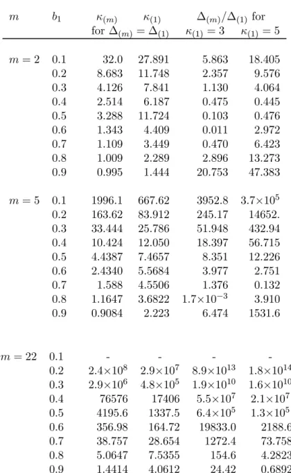
(15) The proof appears in the Appendix. Note that the ratio in (3.6) only depends on two parameters, namely the ARCH persistence parameter b(m),1 and the tail behavior of the ARCH process expressed by κ(m) . The latter two parameters determine the relative local power trade-off.. When ∆(m) /∆(1) equals one then the test exhibits equal local asymptotic power at both sampling frequencies. In such a case the sample size reduction is exactly compensated by persistence/tail behavior trade-off.. In all other circumstances the aggregation implies a decrease in local asymptotic power, when ∆(m) /∆(1) > 1 or an increase when the reverse is true. Solutions to the system of equations (3.6) and (3.7) are presented in Table 1. The different choices of m represent the situations when sampling frequency is doubled m = 2 (e. g. sampling returns mid and end of day), or sampling involves weekly or monthly aggregation, m = 5 and 22, respectively. Two alternative approaches are adopted for solving the system. First we assume that the local asymptotic power is the same irrespective of the sampling frequency ∆(m) = ∆(1) which yields solutions for κ(1) and κ(m) reported in the first two columns (for each m) in Table 1. The results show a clear trade-off between the kurtosis coefficients κ(m) and the persistence coefficient b1 for the m = 2, 5, 22. It is worth noting that the relationship between κ(m) and κ(1) is not monotone. Second we assume a daily kurtosis coefficient κ(1) derived from the empirical evidence of Normality κ(1) = 3 and Student’s t(7) (Bollerslev, 1990) κ(1) = 5 (given that the unconditional t kurtosis is κ = 3 + 6/(ν − 4)) and first solve for κ(m) in (3.7) and then for (3.6). Most solutions yield that ∆(m) /∆(1) > 1 which suggest that asymptotically the local power of the test will be higher for high frequency processes. This is result appears stronger for the ratio at m = 22 as opposed to m = 2.. 4. Sequential CUSUM Test for Volatility Models. Real time monitoring with CUSUM type statistics based on parameter estimates or residuals of static and dynamic linear regression models for economic time series is addressed, for instance, in Chu et al. (1996) and Leisch et al. (2000) and Zeileis et al. (2004). We consider nonlinear time series models proposed for financial asset returns, namely ARCH type processes and our analysis is not strictly parametric in that it can be applied to other strongly. 12.

(16) dependent processes that satisfy the general conditions outlined below. Moreover, we do not consider sequential change-point tests for parameter estimates or residuals of such time series models. Instead our monitoring procedures focus on the observed process and its transformations that are driven by a dynamic volatility model, as well as high frequency volatility estimators that exhibit optimal properties for a general class of GARCH and SV processes. It is important to note at the outset that unlike the residuals of dynamic linear regression models, the residuals of GARCH models do not satisfy the Functional Central Limit Theorem (FCLT) with a Wiener process limit and therefore their boundary crossing probabilities cannot be used. For the location-scale nonlinear time series model in (2.1) we focus on the following general conditional dynamic scale model. A random sequence {Xt , t ∈ T } satisfies the following equations if there exists a sequence of i.i.d. non-negative random variables {ξ t , t ∈ T } such that: Xt = σ(X0t−1 , bj )ξ t , σ(X0t−1 , bj ) = b0 +. t≥1. (4.1). bX j=1 j t−j. (4.2). X∞. where b0 ≥ 0, bj ≥ 0, j = 1, 2, ... The model (4.1)-(4.2) in Robinson (1991) is general enough to include the following ARCH type models: The ARCH(∞) (Engle (1982)) where rt2 = σ 2t u2t , σ 2t = b0 +. X∞. b r2 j=1 j t−j. (4.3). and the Power-ARCH(∞) (Taylor (1986)) |rt |δ = σ δt |ut |δ , σ δt = b0 +. X∞. b |r |δ j=1 j t−j. (4.4). where δ > 0 and ut are i.i.d. random variables with zero mean. Moreover the GARCH(p, q) model rt2 = σ 2t u2t , σ 2t = α0 +. Xp. a σ2 + j=1 j t−j. Xq. j=1. 2 dj rt−j. (4.5). can be rewritten in the form of the ARCH(∞) with positive exponentially decaying bj under some additional constraints on the coefficients aj , dj (Nelson and Cao (1992)). For instance, the GARCH(1,1) model can be rewritten in the form of (4.1)-(4.2) with σ(X0t−1 , bj ) = σ 2t , ξ t = u2t , Xt = rt2 and the coefficients b0 = α0 (1 + α1 + α21 + ...) = α0 /(1 − α1 ), bj = aj−1 1 d1 . 13.

(17) The following parameter and moment condition: E(ξ 20 ) < ∞ and E(ξ 20 ). X∞. b j=1 j. <1. (4.6). for the general specification in (4.1)-(4.2) implies that: (a) {Xt } is strictly and weakly stationary. (b) {Xt } exhibits short memory in the sense that covariance function P is absolutely summable, ∞ t=−∞ cov(Xt , X0 ) < ∞ (Kokoszka and Leipus (2000)). (c) {Xt } satisfies the Functional Central Limit Theorem (FCLT). Giraitis et al. (2000) prove that as N → ∞ SN (t) := N −1/2 P. X[N t] j=1. (Xj − E(Xj )) → σW (t), 0 ≤ t ≤ 1. (4.7). where σ2 = ∞ t=−∞ cov(Xt , X0 ) < ∞ and {W (t), 0 ≤ t ≤ 1} is a standard Wiener process with zero mean and covariance E(W (t)W (s)) = min(t, s). It is interesting to note that the CLT holds without having to impose any other memory restrictions on Xt such as mixing conditions. The reason being that the condition in (4.6) implies not only (a) weak stationarity but also (b) short memory. Kokoszka and Leipus (2000) show that if, in addition, bj decay exponentially then so does the covariance function. Finally, the FCLT for Xt holds without the Gaussianity assumption. The ARCH type models (4.3)-(4.5) can be considered in the context of the general specification (4.1)-(4.2) for which ξ t = f (ut ) for some non-negative function f . Therefore condition (4.6) can lead to corresponding conditions for the above ARCH models. For instance, for the ARCH(∞) model ξ t = u2t P 4 and condition (4.6) becomes E(u40 ) < ∞ and E(u40 ) ∞ j=1 bj < 1. δ The FCLT result for Xt in (4.1)-(4.2) or equivalently |rt | , δ = 1, 2 in (4.3)-(4.5) provides the conditions for deriving the sequential CUSUM tests for dynamic scale models. In contrast to linear dynamic regression models, the residuals of GARCH models do not satisfy the FCLT. Horvath et al. (2001) show that the partial sum of the ARCH(∞) residuals are asymptotically Gaussian, yet involve a covariance structure that is a function of the conditional variance parameters. Therefore the CUSUM test can be applied sequentially to the observed strongly dependent returns and their transformations i.e. Xt = |rt |δ , δ = 1, 2 given that the FCLT conditions (4.6) are 4. Davidson (2000) shows that the FCLT holds for GARCH(p, q) processes based on the sufficient assumptions that ut is i.i.d. with finite fourth moment in the near-epoch dependence framework.. 14.

(18) satisfied. Consequently, boundary crossing probabilities can be computed for the CUSUM test based on Xt as opposed to the ARCH type residuals. Monitoring Xt is equivalent to sequentially testing the stability of dynamic risk measures. Such on-line tests can be considered useful for providing an early warning for a disruption in financial risk which can be considered useful for financial crises. Let us now turn to the derivation of the sequential CUSUM test. Consider a special case of the process Xt in (4.1)-(4.2) as a simple way of specifying the sequential monitoring scheme. The returns process r(m),t sampled at frequency 1/m follows a GARCH(1,1) model: r(m),i,t = σ (m),i,t · u(m),t 2 σ 2(m),i,t = b0,i,(m) + b1,i,(m) r(m),t−1/m + γ i,(m) σ 2(m),i,t−1/m ,. t = 1, ...n, n + 1, ... (4.8) where b0,i,(m) ≥ 0, b1,i,(m) , γ i,(m) > 0 and u(m),t is an i.i.d. zero mean process. 2 Condition (4.6) is applied to u(m),t and the FCLT holds for r(m),t . The subscript i allows for the possibility of a structural change in the volatility process, σ 2(m),i,t . Consider the historical sample t = 1, ..., n where the model is homogeneous such that there are no structural changes i.e. b0,i,(m) = b0,(m) , b1,i,(m) = b1,(m) , γ i,(m) = γ (m) . The objective is to use this historical homogeneous sample to estimate the daily volatility given by σ 2(1),i,t where the subscript (1) refers to the volatility for 1 day. As mentioned above and for uniform notation we will drop the subscript “one” that refers to the sampling frequency when we refer to the daily frequency such that the daily volatility is given by σ 2i,t . It is important to emphasize that we neither estimate the GARCH parameters nor use temporal aggregation of (4.8) and therefore we do not entertain in weak GARCH specifications. Instead we may deal with a strong GARCH and temporally aggregate the high frequency returns process r(m),i,t via intraday sums to obtain data-driven estimators for daily volatility. High frequency volatility estimators are employed in order to filter σ2i,t and we choose to focus on the Power and Quadratic Variations, P Vt and QVt . Other data-driven estimators can also be used. The historical sample t = 1, ..., n is assumed to be homogeneous such that σ 2t is estimated by {P Vt }n1 and {QVt }n1 . The objective is to monitor sequentially new data from time n + 1 onwards to test whether any change-point occurs in σ 2i,t and thereby ri,t during the monitoring period. Hence the sequential test has the following null hypothesis σ (m),i,t = σ (m),t for i > n + 1 against the alternative that at some point in the future the volatility process will change to σ (m),i,t at some 15.

(19) point τ > n.5 Since a break in the unobserved σ (m),i,t implies a change in the observed returns process, r(m),i,t , the following two classes of control processes are considered for sequential testing: (i) The high frequency daily volatility filters {P Vt }n+1 , {QVt }n+1 and (ii) the observed daily returns transformations of {|rt |}n+1 and {rt2 }n+1 . It is worth emphasizing that monitoring with these processes is valid for more general dynamic conditional variance specifications. The alternative approach of estimated parameter-based sequential tests for a strict semiparametric GARCH model is pursued in Berkes et al. (2004) based on Generalized Likelihood Ratio (GLR) tests. The sequential CUSUM test that involves the volatility control processes Xt . The sequential CUSUM test that involves the above control processes can be derived for instance for the daily squared returns process of (4.8). It follows from the FCLT that the partial sum: (T − n)−1/2 σ −1. Xτ T. j=n+1. (rj2 − µ) → W (τ ). (4.9). converges to the Wiener process W . Note that µ = E(rj2 ) and refers to the mean over the respective partial sum. The derivation of the sequential CUSUM test can be found, for instance, in Chu et al. (1996). Take T = λn, then (4.9) is n−1/2 (λ − 1)−1/2 σ −1. Xτ T. j=n+1. (rj2 − ν) → W (τ ).. (4.10). The CUSUM process for monitoring is defined by: . QnT = n−1/2 σ −1 (λ − 1)−1/2. τT X. (rj2 − ν) −. j=n+1. n X. . (rj2 − ν) → B(τ ). j=1. (4.11). if n → ∞ and λ → 2 or t/n → 1, where B(τ ) is a Brownian bridge: . QnT = n−1/2 σ −1 . τT X. (rj2 − ν) −. j=n+1. P. n X. . (rj2 − ν) → B(τ ). j=1. (4.12). 2 2 The variance σ 2 = ∞ j=−∞ cov(rj , r0 ) and a consistent estimator for the longrun variance, e.g. a Heteroskedastic Autocorrelation Consistent (HAC) estimator for rj2 . As mentioned in section 2.2 the ARHAC estimator is used for σ. 5. We assume that the error process u(m),t is homogeneous and does not represent another possible source of change in σ (m),i,t . Such change-point alternatives are considered elsewhere, see for instance Andreou and Ghysels (2003).. 16.

(20) For the sequential CUSUM statistic the theory of the drifted Wiener process provides a way to find the appropriate boundaries. Linear and parabolic boundary functions √ can be √ considered that grow with the sample size at approximately rates t and log t. Certain boundary functions for the Brownian bridge are derived using the Law of Iterated Logarithm √ (LIL). For instance, Khintchine’s LIL shows that the boundary b1 (t) = 2t log log t standardizes the supremum of the Brownian motion. This LIL extends to partial sums of dependent processes (Altissimo and Corradi, 2003, Segen and Sanderson, 1980) and is motivated by the fastest detection of change. However, Altissimo and Corradi (2003) and Chu et al. (1996) show via simulations that in finite samples the probability of type one error is erratic and high for b1 (t). Chu et al. (1996) also extend the i.i.d. results of Robbins and Seigmund (1970) to monitoring procedures where the partial sum of the residuals and recursive estimates in linear time series obey the FCLT, under milder restrictions on general class of boundary functions (see Theorem 3.4, p. 1051 and Theorem A, Appendix A, p. 1062). The following boundary is derived analytically for the sequential CUSUM-type and Fluctuation tests: b2 (t) =. s. t(t − 1). ·. α2. µ. t + ln t−1. ¶¸. (4.13). where α2 = 7.78 and 6.25 gives the 5% and 10% monitoring boundaries, respectively. Revesz (1982) shows that the asymptotic √ growth rate of the supremum of the increments of the Wiener process q is ln t almost surely. Leisch et al. (2000) specify the boundary b3 (t) = λ 2 log+ t where log+ t = 1 if t ≤ e and log+ t = log t if t > e, for which the critical values λ for the increments of a Brownian bridge are obtained via simulations in the context of Generalized Fluctuation tests (see for instance, Table 1, p. q 846, Leisch et al., 2000). Similarly, Altissimo and Corradi (2003) suggest λ 2 ln(ln t) based on the exact distribution of the supremum of a Brownian bridge, where λ is derived via simulation to yield the adjusted bounds (reported in Table 2, Altissimo and Corradi, 2003). Leisch et al. (2000) show that b3 (t) leads to tests that are sensitive to change-points that occur early or late in the monitoring period asqopposed to b2 (t). Zeileis et al. (2004) argue that simulation evidence for λ log+ t suggests most of the size of the test is used at the point where the boundary changes from being constant to growing and this makes it inap17.

(21) propriate for a process with growing variance such as the Brownian bridge. Hence they suggest a simple boundary that has the advantage of not using up the size of the corresponding test at the beginning of the monitoring period while at the same time growing in a linear manner given by b4 (t) = λt. (4.14). where λ is the simulated critical value for alternative monitoring horizons (shown in Table III in Zeileis et al., 2004). In the remainder of the analysis we consider b2 (t) and b4 (t) and note that these linear boundaries cross at some point during the monitoring period. For instance, if the historical sample is n then b2 (t) and b4 (t) cross at 2n for a 10% significance level. After the crossing point the slope of b4 (t) is lower than that of b2 (t) which implies that it is more likely to capture small breaks late in the sample. In contrast, before the crossing point b4 (t) rests higher then b2 (t) which means that the probability to detect an early break is lower for b4 (t) relative to b2 (t). The choice of the boundary in sequential testing is traditionally followed based on the minimization of the average detection delay of the Average Run Length (ARL). Other criteria or the combination of boundaries or the derivation of optimal tests given a boundary are still open questions in the literature.. 5. Simulation evidence for sequential CUSUM. In this section we examine the properties of the sequential CUSUM changepoint test for GARCH processes. The analysis has the following objectives: (i) The finite sample properties of the monitoring procedure are examined for alternative boundaries and volatility filters and daily returns processes. (ii) The effects of heavy tails and persistence in a GARCH on the CUSUM test are examined in conjunction with the local power results in a sequential framework. The results in this section extend existing simulation evidence in the following respects: First, results are presented for the finite sample behavior of the on-line CUSUM test for strongly dependent processes as opposed to the independent models presented in Chu et al. (1996) and Leisch et al. (2000) and linear time series models in Zeileis et al. (2004). Second, supportive evidence is provided for the CUSUM test for monitoring directly the 18.

(22) observed returns process and its transformations as well as high frequency volatility filters instead of adopting a more traditional approach of monitoring the parameter estimates of a volatility model or its residuals. Third, it introduces another important variable in sequential testing namely the sampling frequency and shows how high frequency volatility filters can improve the detection delay of the CUSUM test for GARCH models to rates that are comparable to NIID setups (of Chu et al., 1996 and Leisch et al., 2000).. 5.1. The Monte Carlo design. The simulated returns process r(m),t sampled at frequency 1/m is generated by a GARCH(1,1) model: r(m),t = µ(m),t + σ (m),t · u(m),t 2 σ 2(m),t = b(m),0 + b(m),1 r(m),t−1/m + γ (m) σ 2(m),t−1/m ,. t = 1, ..., T.. (5.1). where u(m),t is i.i.d. N (0, 1) and σ 2(m),t is the volatility process. The Data Generating Processes (DGP) at the 30-minute frequency are: (i) a low persistent GARCH where b(m),0 = 0.038, b(m),1 = 0.056, γ (m) = 0.933 and (ii) a high persistent GARCH b(m),0 = 0.034, b(m),1 = 0.035, γ (m) = 0.96, both of which can be considered representative processes for financial asset returns. Note that at the 30-minute frequency m = 48 for the 24-hour traded markets. Using the 30-minutes returns process in (5.1) we temporally aggregate them to the daily frequency without imposing the assumption that at those frequencies the data are driven by a GARCH process with i.i.d. errors. The reason being that we do not wish to impose the strong GARCH process assumption (Drost and Nijman, 1993) at all frequencies since these do not temporally aggregate. The control processes refer to two classes: (i) the observed daily returns process and its square and absolute transformations, rt2 and |rt | and (ii) high frequency volatility estimators, namely QVt and P Vt . Barndorff-Nielsen and (m) (m) Shephard (2004) show that the asymptotic properties of QVt and P Vt are valid even if m = 48. Under the null, the process in (5.1) is driven by a homogeneous process without breaks in the conditional variance.6 We compute the empirical crossing probabilities under the null for historical sample sizes n = 75, 125, 250, 500 6. It is assumed that µ(m),t = 0 for simplicity. Consequently, we focus on scale change point alternatives that are more challenging to detect as opposed to mean shifts.. 19.

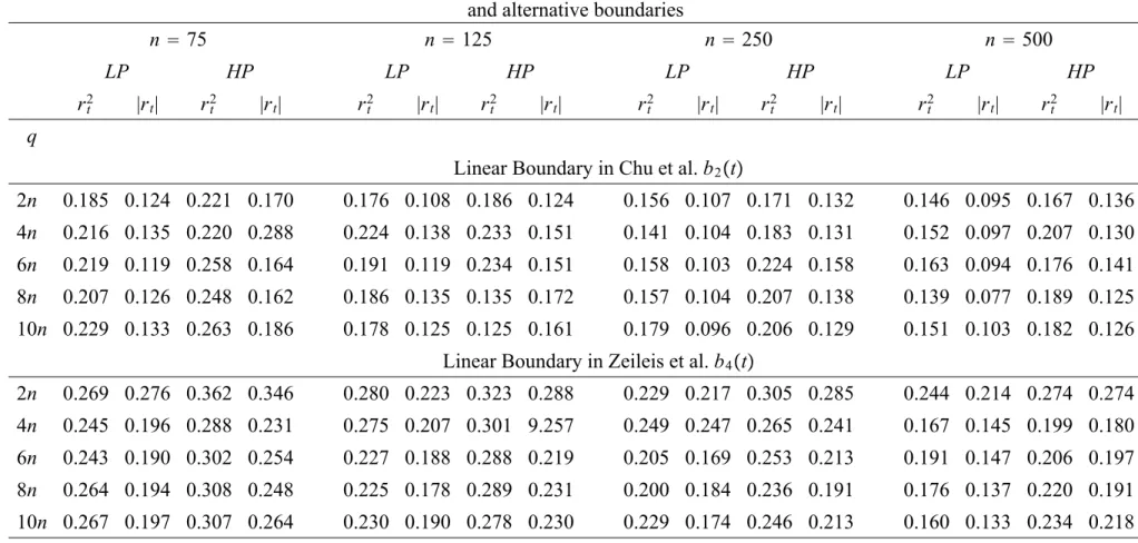
(23) days. The choice of the historical sample takes into account various financial applications e.g. one or two years of daily data are recommended by regulators for estimating risk management measures. Smaller samples can also be considered when there is an end or beginning of sample instability. Such small historical samples are feasible for the control processes considered in the analysis (i.e. daily returns transformations and high frequency volatility filters) but for the estimation of GARCH type models and for monitoring its parameters larger samples are preferred. The monitoring horizon q is set to q = 2n, 4n, 6n, 8n, 10n days. According to the theory if n is large enough and q is extended to infinity the crossing probabilities should approach the nominal size for the given boundaries b2 (t) and b4 (t). Although it is not possible to set q equal to infinity in simulations, the objective is to examine whether there are any size distortions for the above test with various finite values of q. Under the alternative hypothesis the returns process is assumed to exhibit a change-point in the conditional variance, σ (m),t , which can be thought as permanent regime shifts in volatility at an out-of- sample point τ = πn (where π = 1.1 and 3 represent respectively beginning- and end-of-sample instabilities) and q = 10n. Such breaks may be due to an increase in the intercept, b(m),0 , or a shift in the volatility persistence, b(m),1 + γ (m) or both. For both low and high persistent GARCH processes under the change-point regime the constant shifts from b(m),0 to 3b(m),0 and the dynamics from b(m),1 = 0.94 to b(m),1 = 0.91 in the high persistence GARCH and b(m),1 = 0.933 to b(m),1 = 0.91 in the low persistence GARCH. Under the alternative hypothesis it is useful to examine whether the test is consistent i.e. it eventually signals the break, yet it is even more informative to show that the on-line CUSUM, given a boundary, minimizes the detection delay which is defined at the Average Run Length (ARL). Similarly, the empirical distribution of the first hitting time gives a more complete picture of the power properties of the test. All simulation results are based on 1000 trials.. 5.2. Simulation results. The simulation results relating to the size of the sequential CUSUM in (4.12) can be found in Tables 2 and 3 for the two classes of control processes, the daily returns transformations, rt2 and |rt | and the high frequency volatility estimators, QVt and P Vt . The size properties are examined for both low and high persistent GARCH models and for various historical samples, n, 20.

(24) and monitoring horizons, q, as defined above. We examine the two linear boundaries: The Chu et al. b2 (t) boundary in equation (4.13) and the Zeileis et al. boundary b4 (t) in equation (4.14), at the 10% significance level. Table 2 shows that for both low and high persistence GARCH processes and for the two boundaries considered and for the historical sample, n, the size of the on-line test for rt2 and |rt | behaves as follows: • Across boundaries the size of the test improves with large n = 250, 500 and q > 6n. Size distortions are higher for b4 (t) than for b2 (t). The Chu et al. boundary has empirical size close to the nominal even for small n ≥ 125 and q > 2n for |rt | in the context of a low persistence GARCH. For high-persistence GARCH models the CUSUM test yields size distortions almost twice the nominal size and is not recommended for small historical samples of n = 75. • Across control processes the on-line CUSUM has relatively more size distortions for the rt2 than for the |rt | process (with its size being around 5% larger for n = 250, 500). • For the low persistence GARCH process and b2 (t) the |rt | yield empirical size very close to the nominal for different choices of n and q. Table 3 also presents the size of the sequential CUSUM test for the second class of monitoring processes, the high-frequency volatility filters, QVt and P Vt , that behaves as follows: • For the P Vt the size of the sequential CUSUM improves for n ≥ 250 and q ≥ 4n and either boundary. For n = 500 and b2 (t) the size is close to the nominal one. • Across control processes the test has relatively more size distortions for the QVt as opposed to the P Vt process. Comparing the simulated size of the sequential CUSUM for the two classes of monitoring processes we find that the test has less size distortions for the high-frequency volatility filters as opposed to the daily returns transformations. This can be explained by the fact that high-frequency volatility filters are more accurate and smooth estimates of volatility as opposed to the absolute and squared returns. For alternative boundaries, GARCH persistence 21.

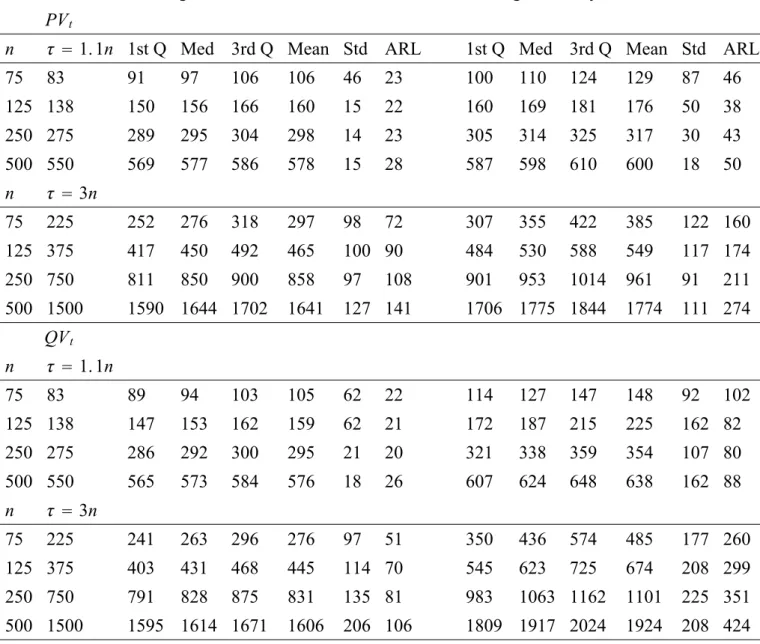
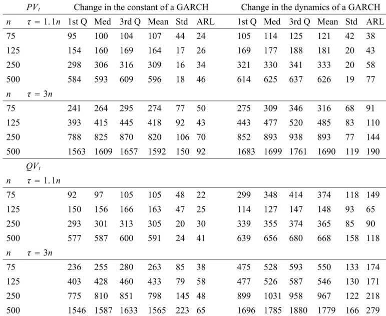
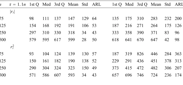
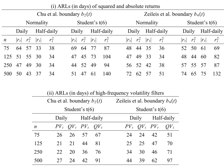
(25) effects, n and q, the monitoring process with size close to the nominal one is |rt | followed by P Vt . For the same parameters the size of rt2 and QVt is on average 1.5 times larger than the nominal one. We now turn to assess the power of the sequential CUSUM test by evaluating the empirical distribution of the first hitting time. These simulation results are also compared across different boundaries, change-point locations and control processes as follows: Properties of ARLs The detection timing or delay is measured by the Average Run Length (ARL). The size and type of break affects the ARL in the following way. Although in the simulation setup both breaks in b0,(m) and b1,(m) lead to the same magnitude of change of the unconditional variance (b0,(m) /(1 − b1,(m) )), the size of change in the constant is of course larger than that of the dynamics of the GARCH. More importantly the break in the constant leads to a level shift whereas a break in the dynamics leads to a trend or slope change which may be relatively more difficult to detect. Hence the ARL is lower when there is a break in the constant as opposed to the dynamics of a GARCH. The simulation results also provide evidence that this result is valid for both linear boundaries, classes of control processes, locations of break and GARCH level of persistence. More specifically we find that when there is a shift in the constant the ARL is half the size of the ARL obtained when there is break in the dynamics of a GARCH. Within the same setup (of control processes, linear boundaries and change-points) the ARLs are small and comparable to the ARLs for the NIID case reported in Chu et al. (Table II). For instance, Table 4 shows that monitoring the P Vt and QVt with the Chu et al. boundary when there is a break at τ = 1.1n in the constant of the GARCH leads to an average ARL of 24 days across n. In the same setup when there is a break in the dynamics of the GARCH the choice of monitoring the P Vt yields a lower average ARL of 44 days as opposed to 90 days when monitoring the QVt . Dispersion of hitting times The standard deviation of the first hitting time decreases significantly for n ≥ 75 for an early change point at τ = 1.1n in the constant of a low persistence GARCH for the QVt and P Vt and for both linear boundaries, as shown in Tables 4 and 7, respectively. The same result holds for the rt2 and |rt | 22.

(26) when n ≥ 250 as shown in Tables 8 and 9. A lower standard deviation implies a lower probability of false alarm. The larger historical sample n ≥ 250 is required to reduce the standard deviation when the underlying GARCH exhibits higher persistence, as shown in Table 5. However, when there is a break in the dynamics of the GARCH the standard deviation of the first hitting time increases dramatically (as opposed to when there is break in the constant) for all processes except for the P Vt and |rt | when τ = 1.1n. Their standard deviation appears stable when n = 500 for an early change-point and for alternative boundaries, persistence effects and types of change-point. This result suggests that the precision of the on-line CUSUM depends on how accurately we estimate the conditional variance in a historical sample. The efficiency of high-frequency volatility filters P Vt and QVt is due to the fact that they exploit the intraday information of returns and have a lower measurement error as opposed to the daily returns processes |rt | and rt2 . On the other hand, the standard deviation appears to be high and does not improve with n when τ = 3n for both control processes and linear boundaries and GARCH models. Choice of volatility filter The above points also imply that one important factor for the power properties of the sequential CUSUM is the choice of monitoring or control process. The historical CUSUM test in Kokoskza and Leipus (2000) is derived for the daily returns transformations rt2 and |rt | from the GARCH model. The simulation results for the sequential CUSUM test for the daily returns processes are shown in Tables 8 and 9 for the Chu et al. and Zeileis et al. boundaries, respectively. The overall results suggest that across n the average ALR is very similar for rt2 and |rt | for the Chu et al. boundary equal to 50 and 53 days, respectively, when there is a break in the constant at τ = 1.1n. For the same setup if we were to consider the industry benchmark for volatility i.e. the RiskMetrics (RMt ) in Table 6 we find that the average ARL increases to 70 days. Even for n = 500 the RMt yields a detection delay of 59 days as opposed to 50 and 43 days for |rt | and rt2 , respectively, when there is a break in the constant at τ = 1.1n. The monitoring processes of high frequency volatility filters lead to the relatively lowest ARLs. For the P Vt and QVt the average ARL is 24 days as shown in Table 4. Similarly they yield the lowest standard deviation of the empirical distribution of the first hitting time among all the control processes 23.

(27) considered. The average standard deviation for b2 (t) and a constant changepoint at τ = 1.1n is 23, 32, 74, 115, 139 days the for P Vt , QVt , |rt |, rt2 , RMt , respectively. Choice of Boundaries One of the most important factors of optimality in sequential testing is the choice of boundaries. In this context we consider the traditional measure of optimality which is the earliest detection timing among two boundaries, b2 (t) and b4 (t). For the early change point at τ = 1.1n and all n the average ALR is very similar for rt2 and |rt | for the two linear boundaries: The ARL is equal to 50 and 53 days, respectively, for b2 (t) and equal to 56 and 51 days, respectively, for b4 (t) when there is a break in the constant. For the same change-point the average ARL for P Vt and QVt is 24 days for b2 (t) and 32 and 27 days, respectively, for b4 (t). These boundaries are also evaluated with respect to the location of the break. The reported simulation results in Chu et al. their sequential test is less effective when τ = 1.2n. This is further evaluated by Leisch et al. for τ = 3n who propose the log boundary b3 (t) that has better properties for end-of-sample instability. Our simulation analysis verifies that when τ = 3n the Chu et al. boundary yields a much higher ARL than the Zeileis et al. boundary which has a lower slope as the monitoring sample increases. For instance, when there is a break in the constant at τ = 3n the average ARL across n is for the P Vt and QVt are 103 and 77 days, respectively, for b2 (t) and 64 and 52 days, respectively, for b4 (t). Similar results extend to the case of monitoring |rt | and rt2 for which the average ARL is at τ = 3n equal to 202 and 156 days, respectively, for b2 (t) and 129 and 119, respectively, for b4 (t). Hence, the Zeileis et al. boundary yields the lowest ARL when used to monitor P Vt and QVt for breaks that occur late in the sample. The symmetry of the empirical distribution of the stopping time is also evaluated for the alternative boundaries. For an early change-point the Chu et al. boundary has a symmetric distribution for the P Vt and QVt for n ≥ 125 and for the rt2 and |rt | for n ≥ 250. The simulated distribution of the first hitting time appears to be relatively less symmetric for the Zeileis et al. boundary.. 5.3. The effects of sampling frequency. The local power analysis for the historical CUSUM test in section 3 shows that the sampling frequency yields some interesting power considerations for 24.

(28) the change-point analysis. Although it is less obvious how to extend these analytical results in a sequential framework given the existence of a nonconstant boundary, we resort to the following simulation analysis in order to obtain some indication of the effects of sampling frequency on the on-line CUSUM. Assuming that locally the boundary is approximately constant we expect from the local power results in section 3 that if we double the sampling frequency of squared returns i.e. sample and thereby monitor twice as often then the power of the test will improve under the assumption of a low persistence ARCH with Normal tails. On the other hand, if the low persistence ARCH exhibits heavy tails then there is a trade-off between sampling frequency and power such that in the presence of a heavy tailed error GARCH the power deteriorates with sampling and monitoring twice more frequently. In order to examine these effects we generate the low persistence GARCH process with Normal and Student’s t(6) errors and examine the ARL for daily and half-daily control processes. If the historical local power results transfer to the sequential framework then we would expect that the ARL would improve when monitoring half-daily squared returns of a Normal GARCH and when monitoring daily squared returns of a Student’s t GARCH. Note that the historical local power analysis in section 3 is derived for the squared returns process but may also extend the simulation analysis to the absolute returns transformation. The simulation results in Tables 10 and 11 present significant evidence that support the historical local power analytical results in the sequential framework. Table 10 presents the simulated size of the absolute and squared returns processes for half-daily monitoring when the 30-minute GARCH process is driven either by Normal or t(6) errors. Compared with the daily monitoring empirical size results in Table 2 we conclude that there are no size distortions from doubling the frequency. Table 11 panel (A) presents the ARLs in days for daily and half-daily monitoring when there is a change point in the constant of a low persistence GARCH process. There is supportive simulation evidence for the following propositions: (i) In the context of a low persistence Normal GARCH sampling and monitoring half-daily improves the ARLs of the CUSUM test for both control processes, rt2 and |rt | and both types of linear boundaries, b2 (t) and b4 (t). Under the Normal GARCH process, the average ARL for the daily monitoring is 51 and 52 days for the daily rt2 , for the Chu et al. and Zeileis et al. boundaries. These ARLs improve when the sampling frequency doubles: The average ARL for the half-daily monitoring is 35 and 40 days for the half-day rt2 , for b2 (t) and 25.

(29) b4 (t), respectively. Similar results are obtained for the |rt | process. However under the Student’s t GARCH process, we obtain the opposite picture, namely the average ARL is 52 and 106 days for daily and half-daily rt2 monitoring, respectively, under b2 (t). Similar results obtain for |rt | and the other boundary. Moreover, these results extend to the high-frequency volatility filters for which we find that there is a strong trade-off between heavy tails and sampling frequency: For a t(6) GARCH process the CUSUM test with either linear boundary, the daily ARLs for both daily P Vt and QVt are approximately half the size of the ARLs for the half-daily high-frequency volatility control processes. Refer, for instance, to the second panel in Table 11.. 6. Prediction-based formulas for earlier detection. The purpose of this section is to present a prediction-based formula that enhances the detection of change points. One of the main challenges of change-point analysis is the reduction of the delay time in detecting breaks. In the previous section we showed that in a sequential framework the CUSUM test signals the instability of the constant in a GARCH process with an ARL that is comparable to the ARLs of independent processes. However, the detection of a small break in the dynamics of a GARCH is more difficult partly due to the nonlinear time series structure of the process. The challenge remains in finding a method or a test that minimizes the detection delay and can be used in the context of prediction analysis. Here we present what is to the best to our knowledge a novel approach in reducing the ARL via a new formula which provides an estimate of the probability that a CUSUM statistic will cross a given boundary over a particular horizon. The formula yielding the probability forecast is based on the extrapolation of the current level of the CUSUM statistic over a particular horizon and exploits the local behavior of a Brownian bridge process. We find that for certain processes this sequential prediction-based method signals the change point earlier than the traditional sequential monitoring statistic. Moreover it also seems to avoid false alarms as under the null the statistic behaves well. We present the formula in a first subsection, followed by simulation evidence reported in a second subsection.. 26.

(30) 6.1. Prediction-based formula. This section presents a simple simulation design for the sequential predictionbased of say qs days ahead which yields the probability that a statistic will exceed a given boundary. The statistic relies on a scaled version of the CUSUM vis-á-vis a future boundary threshold. The approach is different from conventional sequential analysis which relies on the fact that CUSUM statistics have asymptotic distributions that are described by Brownian bridge processes. It is the properties of the Brownian bridge that determine the boundaries in sequential analysis, as discussed in detail in the previous sections. We could view this conventional approach as a global one, in contrast to a local analysis which is pursued here. A Brownian bridge process is determined by the end-points of the path. In conventional sequential analysis the end-point is computed under the null using a pre-monitoring sample consistent estimator. Here, we do not use a long run consistent end-point, but rather a local extrapolation of the process as the end-point of a Brownian bridge process that should approximate the immediate horizon of the CUSUM statistic. The immediate horizon is typically 1, 5 or 10 days, namely the period relevant for most risk management purposes. The idea of the local approximation is to take the current level of the CUSUM statistic and extrapolate its behavior over the short horizon. In particular, suppose that the CUSUM statistic is Qnq0 at a given time point q0 greater than the historical sample n < q0 < τ . Next, consider a prediction horizon defined by q1 , which as noted earlier typically is for instance 5- and 10-days. Then consider: bn = Q q1. Ã q  1. −n q0 − n. !. q0 X. j=n+1. xj −. n X. j=1. . xj . (6.2). which represents the extrapolation of where Qnt will be at horizon q1 . This prediction is based on the scaling of Qnq0 by a factor (q1 − n)/(q0 − n). The re-scaled CUSUM statistic appearing in (6.2) is viewed as the end-point of a Brownian bridge process which describes the behavior of the original CUSUM statistic between q0 and q1 . Given this end-point we take the boundary for the CUSUM statistic, where the boundary is taken from the conventional sequential analysis using the (global) Brownian bridge asymptotics. Given this boundary, we can compute the probability that the CUSUM statistic b n will cross the boundary level at the endtied down between Qnq0 and Q q1 point q1 , denoted Bq1 . This probability can readily be computed (see e.g. 27.

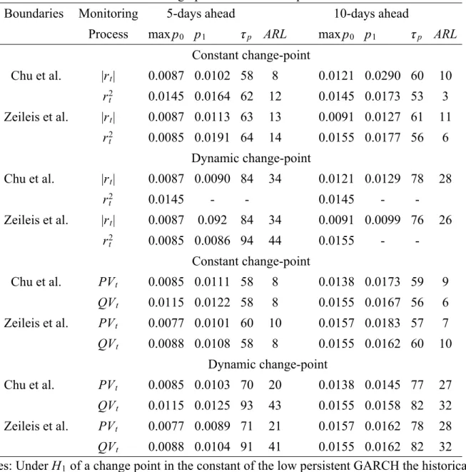
(31) Karatzas and Shreve (1991) or Revuz and Yor (1994)): . . b n ][B − Qn ] 2[Bq1 − Q q1 q1 q0  P ( sup |Qnt | > Bq1 ) = exp − q1 − q0 q0 <t<τ. (6.3). which represents the probability that the CUSUM statistic will exceed the boundary at q1 , i.e. the prediction horizon, given that it is a tied down Brownian motion between its current level and its extrapolated level (6.2). b n and Qn are standardized by the HAC estimator Note that the statistics Q q1 q0 that involves the respective qi sample. It is worth noting that the formula appearing in (6.3) provides certain advantages when compared to the traditional sequential analysis. In particular, it yields a ‘probability statement’ about the likelihood of change-point occurrences. As long as a CUSUM statistic has not crossed a boundary there is no obvious mechanism to make a statement about the likelihood of a break. The formula presented in this section remedies this. It is clear, however, that more work is required on this topic and the purpose of the next subsection is to show that the suggestion to inflate the CUSUM statistic as in (6.2) appears to work. One drawback, however, is that the horizon chosen may be perceived as ad hoc and so does the choice of inflation method for the CUSUM statistic. In addition, we do not have a clear idea yet of the asymptotic distribution of the crossing probabilities under various alternatives. Bootstrapping the probability appearing in (6.3) is one possibility. We leave this subject for future research.. 6.2. Simulation results. We examine the properties of the above sequential predictive statistic using a small simulation design. As in the previous section we first examine the sequential CUSUM test and the ARL for the low persistence GARCH process in 5.1). The results in Table 12 show the ARLs for the two alternative changepoint sources (a break in the constant and the dynamics of a GARCH), the linear boundaries in Chu et al., b2 (t), and Zeileis et al., b4 (t), and the two classes of control processes based on daily returns transformations and high frequency volatility filters. The historical sample involves around one year of daily observations, n = 250, for a total sample of q = 10n observations and the break occurs at τ = 1.5n. It is evident from the results in Table 12 that in all cases the ARLs of the sequential CUSUM statistic as analyzed 28.

(32) in section 5, are relatively high especially for break in the dynamics of a GARCH. Therefore we investigate whether the simple sequential predictionbased formulae in (6.2)-(6.3) result in probability predictions that yield early warning signals of disruptions such that the detection delay is less than that of sequential tests. In the context of the same simulation setup as in Table 12 we set the following parameters: The starting date of the prediction-based analysis is set before the change-point, q0 = 1.3n, the prediction horizons are 5- and 10-days ahead q1 = q0 + pf where pf = 5 or 10 days and the prediction sample is equal to 100 observations. Alternative choices of these parameters are considered in order to robustify the results discussed below. The sequential prediction-based test is simulated under the null and under the two alternative hypotheses of a change-point in the constant and dynamics of a GARCH process. The time series plots of the forecast probabilities are presented. Under the change-point hypothesis the sequential prediction probabilities start trending upwards shortly after the break. For all the above choice parameters of the sequential prediction-based design we find that the daily |rt | instead of rt2 yields the most robust and relatively better prediction-based results as compared with high frequency volatility filters and squared returns. Figures 1 and 2 present the simulated 100 sequential probabilities of |rt | for the 10-days ahead forecasts of the Chu et al. and Zeileis et al. boundaries, respectively. Under the null the sequential probabilities for |rt | fluctuate around a constant mean of 0.007 and 0.005 for b2 (t) and b4 (t), respectively. The maximum simulated probability under the null hypothesis defined by max p0 is presented in Table 13. The maximum of the forecast probabilities under the null for: (i) rt2 does not exceed 0.015 and 0.016 and for (ii) |rt | does not exceed 0.013 and 0.01, for b2 (t) and b4 (t), respectively. Under the alternative hypotheses of a change-point in the constant or the dynamics of a low persistent GARCH process the forecast probabilities, p1 , present dominant trends that deviate from the probabilities under the null as shown in Figures 1 and 2. The interesting feature is that the change in the trend of these forecasts occurs close of the simulated change-point which is observation τ = 50 on the graphs. Although bootstrap confidence intervals are expected to give sharper inferences we may also consider the graphical analysis of these forecasts in relation to their summary in Table 13. For |rt | we find that the forecast probabilities for a change in the constant of a GARCH begin to trend around observation 60 for both types of boundaries and forecast horizons. The top panel of Table 13 shows the exact predicted time, τ p , for which the forecast probabilities of absolute returns, 29.