Ardia : Corresponding author. Département de finance, assurance et immobilier, Université Laval, Québec City,
Québec, Canada; and CIRPÉE
Hoogerheide : Department of Econometrics, Vrije Universiteit Amsterdam, The Netherlands
Forthcoming in Applied Economics Letters. We are grateful to Kris Boudt, Michel Dubois, Ivan Guidotti and Istvan Nagi for useful comments. Any remaining errors or shortcomings are the authors’ responsibility.
Cahier de recherche/Working Paper 13-12
Worldwide Equity Risk Prediction
David Ardia
Lennart F. Hoogerheide
Abstract:
Various GARCH models are applied to daily returns of more than 1200 constituents of
major stock indices worldwide. The value-at-risk forecast performance is investigated for
different markets and industries, considering the test for correct conditional coverage
using the false discovery rate (FDR) methodology. For most of the markets and
industries we find the same two conclusions. First, an asymmetric GARCH specification
is essential when forecasting the 95% value-at-risk. Second, for both the 95% and 99%
value-at-risk it is crucial that the innovations’ distribution is fat-tailed (e.g., Student-t or –
even better – a non-parametric kernel density estimate).
Keywords: GARCH, value-at-risk, equity, worldwide, false discovery rate
1. Introduction
This note investigates the forecasting performance of commonly used GARCH models over a large universe of worldwide equities. Overall, we consider six markets and eleven industries, for a total of more than twelve hundred time series. We rely on a rolling-window estimation approach and forecast the one-day ahead value-at-risk at the 95% and 99% levels for a total of fifteen years of daily data. To our knowledge, this is the first study which performs such a large-scale forecasting performance exercise. The overall backtest study took three days on a eight-core 2GB machine with computationally efficient parallel C++ implementation. This is of substantial importance for risk-management systems, which need to design suitable risk models for many equities. Obviously, practitioners are typically interested in the risk evaluation of portfolios, where one desires to accurately assess the risk in large multivariate settings. However, this does not make the precise evaluation for one asset irrelevant. For example, the validity of copula models depends not only on the validity of the specification of the dependence structure, but also on the validity of the marginal univariate models. For the models, we rely on symmetric and asymmetric specifications for the variance equation and consider Gaussian, Student-t and kernel-based distributions for the errors. The performance of the different models is compared across markets and industries. Our results indicate that an asymmetric specification is essential when forecasting 95% value-at-risk for equities. For both 95% and 99% value-at-risk it is crucial that the innovations’ distribution is fat-tailed. These results are found for most of the markets and industries.
The rest of this note is organized as follows. In section2we present the model specifications, the testing and introduce the false discovery rate method. In section3 we present and discuss the empirical results. Section 4
concludes.
2. Model specification, testing and false discovery rate method
As inMcNeil and Frey(2000), each model considered starts with an AR(1) component in order to filter a possible autoregressive part of the equity log-returns. The models differ in the way the volatility of the error terms is modeled. For that purpose, we rely on the symmetric GARCH(1,1) model ofBollerslev(1986) and on the asymmetric GJR(1,1) model byGlosten et al.(1993). The latter accounts for the asymmetric effect of stock return on next period’s stock return’s variance, known as the leverage effect in the literature (Black,1976).
Both models have a long empirical history and have proved to be successful in volatility modeling in several markets (Bollerslev et al.,1992). They are simple yet powerful GARCH-type models. More specifically, in the GJR model the log-returns rtare expressed as:
rt= µ + ρ rt−1+ ut (t = 1, . . . , T ) ut= σtεt εt∼ iid fε σ2t = ω + (α + γ 1{ut−1≤ 0}) u2t−1+ β σ 2 t−1, (1)
where ω > 0 and α, γ, β ≥ 0 to ensure a positive conditional variance. 1{} denotes the indicator function, whose value is one if the constraint holds and zero otherwise. No constraints have been imposed to ensure covariance stationarity; however, as a sensitivity analysis we have repeated the whole study with additional covariance stationarity constraints, which yielded approximately the same results with qualitatively equal conclusions. Another sensitivity analysis with the inclusion of ‘variance targeting’, where the unconditional variance in the GARCH model is set equal to the sample variance – reducing the number of parameters to be estimated by one, led to similar results. The symmetric GARCH model results by imposing γ = 0. For the distribution fε, we consider the simple Gaussian and Student-t distributions,
together with a non-parametric Gaussian kernel estimator. The Student-t distribution is probably the most commonly used alternative to the Gaussian for modeling stock returns and allows modeling fatter tails than the Gaussian. The kernel approach gives a non-parametric alternative which can deal with skewness and fat tails in a convenient manner. Models are fitted by maximum likelihood. For the non-parametric model, the bandwidth is selected by the rule-of-thumb ofSilverman(1986) on the residuals of the quasi maximum likelihood fit; alternative bandwidth choices lead to similar results. We rely on the rolling-window approach where 1000 log-returns – i.e., approximately four trading years – are used to estimate the models. Similar results were obtained for windows of 750 and 1500 observations. Then, the next log-return is used as a forecasting window. The model parameters are updated every day. At each time point, the one-day ahead value-at-risk forecast is obtained for the different models. Value-at-risk represents the risk
from market movements as one number: the maximum loss expected on an investment, over a given time period at a specific level of confidence. It is nowadays a standard risk measure of downside risk. In our study, the value-at-risk is a negative percentage; in literature it is sometimes quoted as a positive percentage (i.e., a percentile of the distribution for the negative of the return) or an amount of dollars.
To test the ability of our models to capture the true value-at-risk, we compare the realization of the one-day ahead returns rt+1with the value-at-risk estimates (VaR) at 95% and 99% levels. To that aim, we adopt the backtesting
methodology proposed byChristoffersen(1998) which has become the standard practice in financial risk management. This approach is based on the study of the random sequence Vtwhere Vt
.
= 1{rt+1 < VaRt}. A sequence of
value-at-risk forecasts at level (1 − α) has correct conditional coverage if the Vt form an independent and identically
distributed sequence of Bernoulli random variables with parameter α. In practice, this hypothesis can be verified by testing jointly the independence on the series and the unconditional coverage of the VaR forecasts, i.e., E(Vt) = α. We
will estimate the percentage of the time series for which a model provides correct value-at-risk forecasts (in the sense of correct conditional coverage). A naive way to estimate this percentage is to compute the percentage of time series for which the p-value is above a preset significance level, say 5%. However, this approach obviously suffers from Type I errors (rejection for approximately 5% of the time series for which the model performs correctly) and Type II errors (non-rejection for some – or possibly many – of the time series for which the model performs incorrectly). Therefore, the naive estimate may underestimate or overestimate the number of time series for which the model has correct performance, respectively. We therefore correct the percentages of non-rejections using the false discovery rate method ofStorey(2002).
Here the key insight of the false discovery rate method is that in case of a model that delivers correct forecasts for a certain time series the p-value is uniformly distributed between zero and one (see, e.g.Barras et al.,2010). Otherwise, the p-value has an unknown distribution, which should be relatively close to zero. Let λ be the separating value such that for p-values above λ, it is almost certain that they correspond to the null of a correctly performing model. By the properties of the uniform distribution, we can therefore extrapolate the true number of correctly performing models from the p-values exceeding the λ threshold. We rely on the bootstrap method proposed byBarras et al.(2010) to determine the optimal value of λ in a purely data driven way.
3. Results and discussion
We test the performance of the models on constituents of major equity markets worldwide. We consider the regions USA, Western Europe, Asia, South America, Eastern Europe, Middle East and Africa. For each market, all stock constituents of the representative index are considered (using the constituents as of July 2010) for a period ranging from January 1, 1995, to December 31, 2009, thus representing 15 years of daily data. This leads to a database of 3657 equities for which the adjusted daily closing prices are downloaded. The data are then filtered for liquidity followingLesmond et al.(1999). In particular, we remove the time series with less than 1500 data points history, with more than 10% of zero returns and more than two trading weeks of constant price. This filtering approach reduces the database to 1260 time series (around 34% of the overall data set). All data sets are downloaded from Bloomberg. Tables1and2 report a summary of the data used in our analysis. We have chosen this filter, which is obviously rather restrictive since it removes many data series, for the following reasons. First, our aim is a large scale backtest exercise. For this we need a coherent universe of data, where the ‘quality’ of the daily return series should not be too different among regions; this is obtained with the filter. Second, we want to analyze the risk of volatility, not liquidity. Third, the filtered data set represents a universe of stocks where an automated risk management system may be sensible. Nevertheless, we have performed a sensitivity analysis with a different, less stringent filter that led to a smaller reduction of the number of data series; once again, the results were similar.
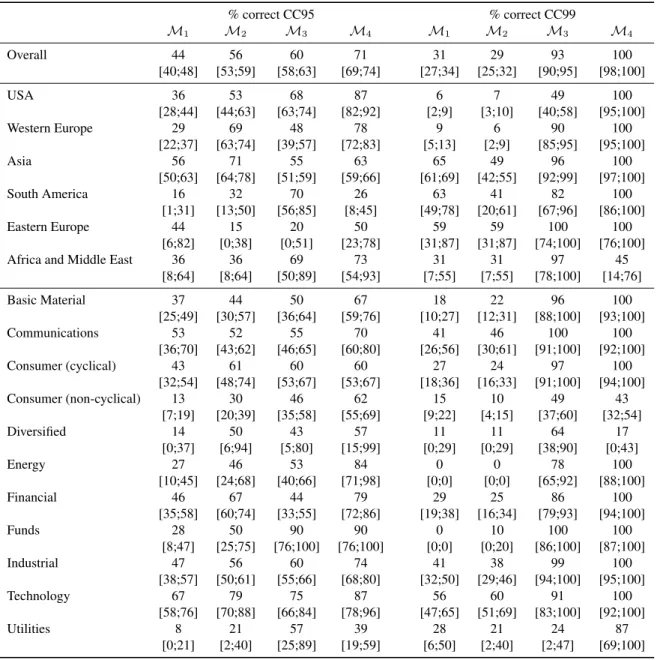
Forecasting results are reported in Table3. For most of the markets and industries we find the same two conclu-sions. First, an asymmetric GARCH specification is essential when forecasting the 95% value-at-risk; the Gaussian GJR model outperforms its symmetric counterpart, the Gaussian GARCH model. On the other hand, when forecast-ing the 99% value-at-risk the Gaussian GJR model does not outperform the Gaussian GARCH model. Second, for both the 95% and 99% value-at-risk it is crucial that the innovations’ distribution is fat-tailed (e.g., Student-t or a non-parametric kernel density estimate).
Especially for the 99% value-at-risk the performance of the GJR model with kernel density estimate of the inno-vations’ distribution is remarkable: for the merged population (and most of the markets and industries) the model may
Market # equities % total USA 297 23.6 Western Europe 288 22.8 Asia 477 37.9 South America 90 7.1 Eastern Europe 45 3.6 Africa & Middle East 63 5.0
Total 1260 100
Table 1: Datasets. Number of time series used in the analysis for each market. USA: S&P 500; Western Europe: EuroStoxx 600; Asia: HSCEI (China), HSI (Hong-Kong), KOSPI (South Korea), SENSEX (Bombay), FSSTI (Singapore), TWSE (Taiwan), TPX 100 (Japan); South America: IBOV (Brazil), MEXBOL (Mexico); Eastern Europe: RTSI$ (Russia), XU100 (Turkey), WIG (Poland); Middle East and Africa: JALSH (South Africa), HERMES (Egypt), DFMGI (Dubai).
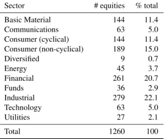
Sector # equities % total Basic Material 144 11.4 Communications 63 5.0 Consumer (cyclical) 144 11.4 Consumer (non-cyclical) 189 15.0 Diversified 9 0.7 Energy 45 3.7 Financial 261 20.7 Funds 36 2.9 Industrial 279 22.1 Technology 63 5.0 Utilities 27 2.1 Total 1260 100
Table 2: Data sets. Number of time series used in the analysis for each sector, as defined by Bloomberg.
yield correct value-at-risk forecasts for the time series of all stock returns. For the 95% value-at-risk the GJR model with kernel is correct for less than 75% of the series. Therefore, an alternative model (e.g., EGARCH, stochastic volatility or regime-switching) or an other estimation method (e.g., Bayesian inference) is required if we desire a correctly performing model for more than 75% of all time series.
We now take a look at the different markets. We see a clear difference between the following two ‘groups’ of regions: (i) USA and Western Europe; (ii) Asia, South America, Eastern Europe, Africa and Middle East. For ‘group’ (i) the GJR model with kernel-based errors is clearly the best model for both 95% and 99% value-at-risk. On the other hand, for ‘group’ (ii) the best model may also be one of the other three models. For Asia and South America the estimated percentage of time series for which the GJR-kernel model provides correct 95% value-at-risk forecasts is lower than the percentage for the GJR model with Gaussian or Student-t errors, respectively. For Eastern Europe, Africa and Middle East the 90% confidence intervals for different models overlap. The GJR-kernel model performs better for (i) than for (ii), arguably because appropriately modeling the properties (i.e., the dynamics and distributions) of stock returns in (ii) is more difficult.
We also consider the different sectors. The GJR model with kernel-based errors performs well for the 99% value-at-risk, except for the ‘Consumer (non-cyclical)’ sector (and ‘Diversified’ but this contains only 9 stocks here). If we compare this model’s prediction quality across the sectors for the 95% value-at-risk, then the worst performance is found for the sectors ‘Consumer (cyclical)’ and ‘Consumer (non-cyclical)’ (except for ‘Diversified’ and ‘Utilities’, where the latter consists of merely 27 stocks). These results suggest that stock returns in the ‘Consumer’ sector(s) have characteristics that are modeled less easily.
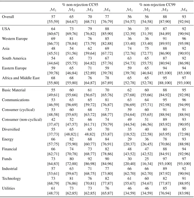
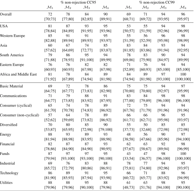
For comparison, Tables 4and5 show the naive estimation results, the percentage of non-rejections at 5% and 1% significance level, respectively. The relatively low percentage of non-rejections — 93% (96%) in Table4(5), as compared with 100% in Table3— for the 99% value-at-risk forecasts from the GJR model with kernel-based error distribution (M4) is possibly caused by a Type I error for 7% (4%) of the time series. The relatively high percentage
of non-rejections — 56% (69%), as compared with 31% in Table3 — for the 99% value-at-risk forecasts from the GARCH model with Gaussian error distribution (M1) is possibly caused by a Type II error for more than 25% (38%)
of the time series. Obviously, Type I errors are more harmful in Table4, whereas Table5suffers more from Type II errors.
4. Conclusion
Various GARCH models are fitted to daily returns of more than 1200 constituents of major stock indices world-wide. The value-at-risk forecast performance is investigated for different markets and industries, considering the test for correct conditional coverage using the false discovery rate methodology. For most of the markets and industries we find that an asymmetric GARCH specification is essential when forecasting the 95% value-at-risk. Moreover, for both the 95% and 99% value-at-risk it is crucial that the innovations’ distribution is fat-tailed (e.g., Student-t or – even better – a non-parametric kernel density estimate).
In future research, we intend to consider the performance of Bayesian estimation and alternative model specifi-cations, extending the analysis ofHoogerheide et al.(2012), who only analyze two data series of stock index returns (S&P 500 and Nikkei 225), and using the methods ofHoogerheide et al.(2007) andHoogerheide and Van Dijk(2010).
References
Barras, L., Scaillet, O., Wermers, R., 2010. False discoveries in mutual fund performance: Measuring luck in estimated alphas. Journal of Finance 65, 179–216.
Black, F., Jan.–Mar. 1976. The pricing of commodity contracts. Journal of Financial Economics 3 (1–2), 167–179.
Bollerslev, T., Apr. 1986. Generalized autoregressive conditional heteroskedasticity. Journal of Econometrics 31 (3), 307–327.
Bollerslev, T., Chou, R. Y., Kroner, K., Apr.–May 1992. ARCH modeling in finance: A review of the theory and empirical evidence. Journal of Econometrics 52 (1–2), 5–59.
Christoffersen, P. F., Nov. 1998. Evaluating interval forecasts. International Economic Review 39 (4), 841–862.
Glosten, L. R., Jaganathan, R., Runkle, D. E., Dec. 1993. On the relation between the expected value and the volatility of the nominal excess return on stocks. Journal of Finance 48 (5), 1779–1801.
Hoogerheide, L. F., Ardia, D., Corr´e, N., 2012. Density prediction of stock index returns using GARCH models: Frequentist or Bayesian estimation? Economics Letters 116 (3), 322–325.
Hoogerheide, L. F., Kaashoek, J. F., Van Dijk, H. K., 2007. On the shape of posterior densities and credible sets in instrumental variable regression models with reduced rank: an application of flexible sampling methods using neural networks. Journal of Econometrics 139 (1), 154–180. Hoogerheide, L. F., Van Dijk, H. K., 2010. Bayesian forecasting of value at risk and expected shortfall using adaptive importance sampling.
International Journal of Forecasting 26 (2), 231–247.
Lesmond, D. A., Ogden, Joseph, P., Trzinka, C. A., 1999. A new estimate of transaction costs. The Review of Financial Studies 12 (5), 1113–1141. McNeil, A. J., Frey, R., Nov. 2000. Estimation of tail-related risk measures for heteroscedastic financial time series: an extreme value approach.
Journal of Empirical Finance 7 (3–4), 271–300.
Silverman, B. W., 1986. Density Estimation for Statistics and Data Analysis, 1st Edition. Chapman and Hall, New York, USA. Storey, J., 2002. A direct approach to false discovery rates. Journal of the Royal Statistical Society B 64, 479–498.
% correct CC95 % correct CC99 M1 M2 M3 M4 M1 M2 M3 M4 Overall 44 56 60 71 31 29 93 100 [40;48] [53;59] [58;63] [69;74] [27;34] [25;32] [90;95] [98;100] USA 36 53 68 87 6 7 49 100 [28;44] [44;63] [63;74] [82;92] [2;9] [3;10] [40;58] [95;100] Western Europe 29 69 48 78 9 6 90 100 [22;37] [63;74] [39;57] [72;83] [5;13] [2;9] [85;95] [95;100] Asia 56 71 55 63 65 49 96 100 [50;63] [64;78] [51;59] [59;66] [61;69] [42;55] [92;99] [97;100] South America 16 32 70 26 63 41 82 100 [1;31] [13;50] [56;85] [8;45] [49;78] [20;61] [67;96] [86;100] Eastern Europe 44 15 20 50 59 59 100 100 [6;82] [0;38] [0;51] [23;78] [31;87] [31;87] [74;100] [76;100] Africa and Middle East 36 36 69 73 31 31 97 45
[8;64] [8;64] [50;89] [54;93] [7;55] [7;55] [78;100] [14;76] Basic Material 37 44 50 67 18 22 96 100 [25;49] [30;57] [36;64] [59;76] [10;27] [12;31] [88;100] [93;100] Communications 53 52 55 70 41 46 100 100 [36;70] [43;62] [46;65] [60;80] [26;56] [30;61] [91;100] [92;100] Consumer (cyclical) 43 61 60 60 27 24 97 100 [32;54] [48;74] [53;67] [53;67] [18;36] [16;33] [91;100] [94;100] Consumer (non-cyclical) 13 30 46 62 15 10 49 43 [7;19] [20;39] [35;58] [55;69] [9;22] [4;15] [37;60] [32;54] Diversified 14 50 43 57 11 11 64 17 [0;37] [6;94] [5;80] [15;99] [0;29] [0;29] [38;90] [0;43] Energy 27 46 53 84 0 0 78 100 [10;45] [24;68] [40;66] [71;98] [0;0] [0;0] [65;92] [88;100] Financial 46 67 44 79 29 25 86 100 [35;58] [60;74] [33;55] [72;86] [19;38] [16;34] [79;93] [94;100] Funds 28 50 90 90 0 10 100 100 [8;47] [25;75] [76;100] [76;100] [0;0] [0;20] [86;100] [87;100] Industrial 47 56 60 74 41 38 99 100 [38;57] [50;61] [55;66] [68;80] [32;50] [29;46] [94;100] [95;100] Technology 67 79 75 87 56 60 91 100 [58;76] [70;88] [66;84] [78;96] [47;65] [51;69] [83;100] [92;100] Utilities 8 21 57 39 28 21 24 87 [0;21] [2;40] [25;89] [19;59] [6;50] [2;40] [2;47] [69;100]
Table 3: Estimated percentage of the time series for which the model provides correct value-at-risk forecasts (in the sense of correct conditional coverage) for the 95% (CC95) and 99% (CC99) value-at-risk. Percentages are computed from the individual tests’ p-values using the false discovery
rate approach ofStorey(2002). []: asymptotically valid 90% confidence bands derived inBarras et al.(2010). M1: GARCH with Gaussian errors;
% non-rejection CC95 % non-rejection CC99 M1 M2 M3 M4 M1 M2 M3 M4 Overall 57 65 70 77 56 56 88 93 [55;59] [64;67] [68;71] [76;79] [54;57] [54;58] [87;90] [92;94] USA 64 73 79 88 36 35 87 92 [60;67] [69;76] [76;82] [85;90] [32;39] [31;39] [84;89] [90;94] Western Europe 69 81 76 85 36 36 91 96 [66;73] [78;84] [73;79] [82;88] [33;40] [33;40] [89;93] [95;98] Asia 48 54 62 69 74 75 88 92 [45;51] [51;56] [59;64] [67;72] [72;76] [72;77] [86;90] [90;93] South America 54 65 73 67 63 65 87 92 [44;64] [55;75] [64;82] [57;76] [54;73] [55;75] [80;94] [86;98] Eastern Europe 59 65 71 59 59 65 94 94 [39;78] [46;84] [52;89] [39;78] [39;78] [46;84] [85;100] [85;100] Africa and Middle East 68 68 76 78 65 65 95 97
[55;80] [55;80] [64;87] [67;89] [52;78] [52;78] [88;100] [93;100] Basic Material 55 60 61 70 62 60 88 95 [49;61] [55;66] [56;67] [65;76] [57;68] [55;66] [84;92] [92;98] Communications 53 63 65 81 63 64 95 96 [46;59] [56;69] [59;72] [76;87] [56;69] [57;71] [92;98] [94;99] Consumer (cyclical) 53 60 68 73 59 60 91 91 [48;58] [55;65] [63;72] [68;77] [54;64] [55;65] [88;94] [88;94] Consumer (non-cyclical) 42 52 66 74 49 51 89 93 [37;47] [47;57] [61;71] [70;79] [44;54] [46;56] [85;92] [90;95] Diversified 55 65 65 70 35 40 80 85 [37;73] [48;82] [ 48;82] [53;87] [18;52] [22;58] [65;95] [72;98] Energy 66 82 68 84 29 36 78 93 [57;75] [75;90] [60;77] [76;91] [20;37] [26;45] [70;86] [88;98] Financial 66 74 73 82 48 47 88 94 [62;71] [70;78] [68;77] [78;86] [43;52] [42;52] [84;91] [92;96] Funds 73 80 92 90 30 25 97 97 [64;83] [72;88] [86;98] [84;96] [20;40] [16;34] [93;100] [93;100] Industrial 57 63 71 77 66 66 89 92 [53;61] [59;67] [68;75] [73;80] [62;70] [62;70] [87;92] [90;94] Technology 73 81 76 82 61 60 82 91 [68;79] [76;86] [70;81] [77;87] [55;67] [54;67] [77;87] [88;95] Utilities 61 73 73 76 46 46 85 90 [48;73] [62;85] [62;85] [65;87] [34;59] [34;59] [76;94] [83;98]
Table 4: Naive estimation: percentage of non-rejections at the 5% level of the conditional coverage test ofChristoffersen(1998) for the 95% (CC95)
and 99% (CC99) value-at-risk. []: asymptotically valid 90% confidence bands with naive standard deviation of a proportion. M1: GARCH with
Gaussian errors; M2: GJR with Gaussian errors; M3: GJR with Student-t errors; M4: GJR with kernel-based errors.
% non-rejection CC95 % non-rejection CC99 M1 M2 M3 M4 M1 M2 M3 M4 Overall 72 78 84 90 69 71 94 96 [70;73] [77;80] [82;85] [89;91] [68;71] [69;72] [93;95] [95;97] USA 81 87 93 95 53 55 94 98 [78;84] [84;89] [91;95] [93;96] [50;57] [51;59] [92;96] [96;99] Western Europe 85 91 91 95 55 56 96 98 [82;88] [89;94] [89;93] [93;97] [51;59] [52;59] [95;98] [98;99] Asia 60 67 74 85 83 84 93 94 [57;62] [64;69] [72;77] [83;87] [81;85] [83;86] [91;94] [92;95] South America 79 86 95 94 78 83 90 94 [71;88] [78;93] [91;100] [89;99] [69;86] [75;90] [84;97] [89;99] Eastern Europe 76 76 82 82 71 76 94 94 [60;93] [60;93] [67;98] [67;98] [52;89] [60;93] [85;100] [85;100] Africa and Middle East 81 78 84 89 84 89 97 100
[71;92] [67;89] [74;94] [81;98] [74;94] [81;98] [93;100] [100;100] Basic Material 69 72 78 86 75 75 94 97 [64;75] [67;77] [73;83] [82;90] [70;80] [70;80] [92;97] [95;99] Communications 71 79 88 91 83 84 98 98 [64;77] [73;85] [83;92] [87;95] [77;88] [79;89] [96;100] [96;100] Consumer (cyclical) 65 74 78 89 72 75 94 94 [61;70] [70;78] [74;83] [86;92] [67;76] [71;79] [91;96] [91;96] Consumer (non-cyclical) 57 64 78 89 66 66 96 95 [52;62] [59;69] [73;82] [86;92] [61;71] [62;71] [95;98] [93;97] Diversified 70 80 85 90 55 50 85 85 [53;87] [65;95] [72;98] [79;100] [37;73] [32;68] [72;98] [72;98] Energy 88 93 89 93 48 56 90 97 [81;94] [88;98] [83;95] [88;98] [38;58] [47;66] [85;96] [94;100] Financial 82 87 87 93 62 63 92 98 [78;86] [84;90] [84;90] [90;95] [57;67] [58;67] [89;94] [96;99] Funds 87 97 97 95 43 47 98 100 [79;94] [93;100] [93;100] [90;100] [33;54] [36;57] [96;100] [100;100] Industrial 69 76 83 88 78 77 94 95 [65;72] [72;79] [80;86] [86;91] [75;81] [74;80] [92;96] [93;97] Technology 86 89 91 95 66 71 88 96 [81;90] [85;93] [87;94] [93;98] [60;72] [65;77] [83;92] [94;99] Utilities 88 88 95 88 61 63 98 95 [79;96] [79;96] [90;100] [79;96] [48;73] [51;76] [94;100] [90;100]
Table 5: Naive estimation: percentage of non-rejections at the 1% level of the conditional coverage test ofChristoffersen(1998) for the 95% (CC95)
and 99% (CC99) value-at-risk. []: asymptotically valid 90% confidence bands with naive standard deviation of a proportion. M1: GARCH with