A better assessment of the recoverable energy behind a body by the exergy method

A velocity decomposition method for exergy-based drag

prediction

Accepté AIAA Journal, mai 2020

Miguel Angel Aguirre1, Sébastien Duplaa2, Xavier Carbonneau3 and Andrew Turnbull4

ISAE-SUPAERO, Toulouse University, 31055, France Safran Tech, 78117, Magny-les-Hameaux, France

The exergy method is a powerful tool for aerodynamic analysis and drag prediction. However, its formulation still requires further improvements in order to obtain a useful drag breakdown for the analysis of wind tunnel data (like the field methods). The far-field drag breakdown is achieved by using a velocity decomposition technique but the related formulation is not well suited for the exergy method. Thus, the main objective of this work is to develop a new velocity decomposition suited for the exergy analysis and to propose a related exergy-based drag breakdown formulation for wind tunnel applications.

Nomenclature

a = speed of sound, m.s-1

CD = drag coefficient c = airfoil chord, m

cv = mass specific heat at constant volume, J.kg-1.K-1

D = drag force, N

𝐸̇𝑢 = axial kinetic exergy, W

1

PhD candidate, Safran Tech; miguel-angel.aguirre@safrangroup.com

2 _{Associate professor, DAEP-Department of Aerodynamics, Energetics and Propulsion;Sebastien.DUPLAA@isae.fr} 3 _{Professor, DAEP-Department of Aerodynamics, Energetics and Propulsion; xavier.carbonneau@isae.fr}

𝐸̇𝑣 = transverse kinetic exergy, W

𝐸̇𝑝 = pressure exergy, W

e = mass specific internal energy, J.kg-1

𝜀̇𝑚 = mechanical exergy outflow rate across the survey plane, W

𝜀̇𝑡ℎ = thermal exergy outflow rate, W

ht = mass specific total enthalpy, J.kg-1

i, j ,k = unit vectors along the aerodynamic x-, y- and z-axes

M = Mach number (= 𝑢0/𝑎0)

n = 𝑛𝑥 i, 𝑛𝑦 j, 𝑛𝑧 k, local surface normal

Ps, Pt = static and total pressure, Pa

Re = Reynolds number (= 𝜌0 𝑢0 c / 𝜇0)

S = surface, m2

s = mass specific entropy, J.kg-1.K-1

Ts, Tt = static and total temperatures, K V = ui, vj, wk, local velocity vector, m.s-1 ()∗ _{= isentropic (inviscid) component}

()̅ = non-isentropic (viscous) component

Greek symbols

α = angle of attack, Degrees

β = angle of sideslip, Degrees

δ( ) = ( ) – ( )0, local variation of a parameter respect to the upstream value

γ = ratio of specific heats

θ = elevation angle, Degrees

μ = dynamic viscosity, kg.m-1.s-1

Ψ = stream function, m2.s-1

ρ = air density, kg.m-3

𝜏̿ = viscous stress tensor, Pa

Subscripts

0 = upstream values b = body

ref = reference

out = outlet section

p = profile drag

w = wake

I.

Introduction

HE characteristic curves of airfoils, wings or any other body are classically obtained by CFD or wind tunnel testing. In a CFD environment, near-field and far-field methods [1, 2] have become a standard analysis tools for both the industry and the research domains. Wind tunnel testing is more demanding for the analysis since a limited amount of parameters and measurements points can be obtained during a wind tunnel run. This has led to the development of far-field formulations where only wake data is required to perform drag calculations [3-7].

Another powerful and promising method is the exergy analysis. This technique has been used during the last 20 years for external aerodynamic analysis, mostly in CFD and analytical applications [8-21]. Particularly, the formulation proposed by Arntz [13] represents a major milestone in the development of the exergy method. Since it requires integrating data in an infinite survey plane, it is well suited for CFD analysis, but this prevents its direct application in a wind tunnel environment. In order to reduce the exergy calculations to the wake region only, a major reformulation must be made. Very few works attempting to calculate the exergy parameters by only measuring the wake parameters have been published [15-21]. Nevertheless, it still lacks a formulation directly related to the Arntz method and capable of providing all the exergy and anergy components inside the wake. Hence, the present work proposes a solution to this problem by adapting a technique already used by the far-field method to reduce data to the wake: the velocity decomposition technique.

II.

Review of the aerodynamic assessment methods

First, the system of reference will be described, then the straightforward near-field method is presented, followed by the wind-tunnel most-suited formulation and finally the exergy method.

A. System of reference

The reference system used hereafter is shown in Fig. 1. It has the x-axis aligned with the upstream flow direction and pointing rearwards, the y-axis points towards the right-hand side of the body and the z-axis points upwards. Moreover, when control volume formulations are used, it is assumed that the outlet section “Sout” of the control volume is a plane (called “survey plane”) and it is placed normal to the x-axis. Also, the lateral surfaces are considered parallel to the upstream direction and far away from the body.

Fig. 1 Conventional reference frame. B. Near-field method

The near field method is the classical approach used in order to obtain the total drag force “D” that’s acting upon a body [1,2]. It takes into account the pressure and viscous forces:

𝐷 = ∫ (𝑃_𝑆𝑏 𝑠 𝑛⃗⃗⃗⃗ − 𝜏̿ . 𝑛𝑥 ⃗⃗⃗⃗ ) 𝑑𝑆𝑥 𝑏 (1)

C. Far-field method

The far-field method applies the momentum conservation equation to a control volume surrounding the body. Several variants of this method are available [3-7], enabling the extraction of the drag force by only analyzing the wake of a body. This paper only uses the Meheut’s method [7] because it is the most accurate for the wind tunnel measurement of stationary flows. It is based on the small perturbations method and the decomposition of the axial velocity deficit inside the wake. This leads to the following profile drag equation:

𝐷𝑝 𝑀𝑒ℎ𝑒𝑢𝑡=𝜌0 𝑢0 2 2 ∫ [− 2 𝛾 𝑀₀2𝛥𝑃𝑡 − 𝛥𝑇𝑡+ (1 − 𝑀02 4 ) 𝛥𝑇𝑡 2_{− 𝛥𝑃} 𝑡 𝛥𝑇𝑡− (1 − 𝑀02)(𝛥𝑢̅2+ 2 𝛥𝑢∗ 𝛥𝑢̅)] 𝑑𝑆 𝑆𝑤 (2) Where: 𝛥𝑃𝑡=_𝑃𝑃𝑡 𝑡0− 1 (3)

𝛥𝑇𝑡=_𝑇𝑇𝑡 𝑡0− 1 (4) 𝛥𝑢 = _𝑢𝑢 0− 1 (5) 𝛥𝑢∗_{= √1 −} 2 (𝛾−1) 𝑀02(( 𝑃𝑠 𝑃_𝑠0) (𝛾−1) 𝛾 − 1) − 𝑣2 _𝑢+ 𝑤2 02 − 1 (6) 𝛥𝑢̅ = 𝛥𝑢 − 𝛥𝑢∗ ₍₇₎

The “small perturbation” assumption considers that the variations of total pressure ΔPt, total temperature ΔTt and axial velocity Δu are small. Moreover, the velocity perturbation Δu is decomposed into an isentropic component Δu∗

and a non-isentropic part Δu̅. The latter is related to the viscous and wave losses (which are sources of entropy, that’s why it is called non-isentropic). Note that Δu̅ is null outside the wake of a body.

For 2D applications, the profile drag is the total drag acting upon a body. For 3D cases, the vortex drag must also be considered:

𝐷𝑣𝑜𝑟𝑡𝑒𝑥= ∫_{𝑆𝑜𝑢𝑡}𝜌₂(𝑣2+ 𝑤2) 𝑑𝑆 (8)

𝐷𝑡𝑜𝑡𝑎𝑙= 𝐷𝑝𝑟𝑜𝑓𝑖𝑙𝑒+ 𝐷𝑣𝑜𝑟𝑡𝑒𝑥 (9)

Throughout this paper, the survey plane position used for the evaluation of the far-field drag values will be placed at 1 chord downstream of the airfoil or wing.

D. Exergy method

Exergy is a classical thermodynamic concept based on the 1st and 2nd laws of thermodynamics [22, 23]. It decomposes the total energy of a system into two components: the exergy “ε” (the useful part of the energy) and the anergy “𝒜” (its useless part). The exergy concept states that any perturbation of the system (perturbation of speed, pressure or temperature) has an inherent energetic potential that can be completely converted into work if the perturbation is returned to its original (equilibrium) state by means of a reversible transformation. If this transformation is irreversible, only one part of this work potential will be recovered. This can be expressed as follows:

The Arntz formulation will be used throughout this paper [13]. It provides an exergy-based drag force equation when an unpowered and adiabatic case is considered:

𝐷 ∗ 𝑢0= 𝒜̇ + 𝜀̇𝑚+ 𝜀̇𝑡ℎ (11)

Each term on the right-hand side represents an equation itself as indicated as follows. Note: the original

equations from Arntz require performing an integral on the entire control volume surface enclosing the body (i.e., S0+Slateral+Sout in Fig.1). Here, the equations have been slightly modified in order to limit the integration to the

outlet surface only (infinite survey plane downstream of the body).

𝒜̇ = 𝑇_𝑠0∫_{𝑆𝑜𝑢𝑡}𝜌 𝛿𝑠 (𝑉⃗ . 𝑛⃗ ) 𝑑𝑆 (12) 𝛿𝑠 = 𝑐𝑝 𝑙𝑛 (_𝑇𝑇𝑠 𝑠0) − 𝑅 𝑙𝑛 ( 𝑃_𝑠 𝑃_𝑠0) (13) 𝜀̇𝑚= ∫_{𝑆𝑜𝑢𝑡}1₂𝜌 𝛿𝑢2(𝑉⃗ . 𝑛⃗ )𝑑𝑆+ ∫_{𝑆𝑜𝑢𝑡}1₂𝜌(𝑣2+ 𝑤2)(𝑉⃗ . 𝑛⃗ )𝑑𝑆+ ∫_{𝑆𝑜𝑢𝑡}(𝑃𝑠− 𝑃_𝑠0)[(𝑉⃗ − 𝑉⃗ 0). 𝑛⃗ ]𝑑𝑆 (14) 𝐸̇𝑢 𝐸̇𝑣 𝐸̇𝑝 𝜀̇𝑡ℎ= 𝜀̇_{𝑡ℎ𝑡𝑒𝑚𝑝𝑒𝑟𝑎𝑡𝑢𝑟𝑒}+ 𝜀̇_{𝑡ℎ𝑝𝑟𝑒𝑠𝑠𝑢𝑟𝑒} (15) 𝜀̇_{𝑡ℎ𝑡𝑒𝑚𝑝𝑒𝑟𝑎𝑡𝑢𝑟𝑒}= ∫ 𝜌 𝑐𝑣 𝑇𝑠 (𝑉⃗ . 𝑛⃗ ) [1 − 𝑇_𝑠0 𝑇_𝑠 𝑙𝑛 ( 𝑇_𝑠 𝑇_𝑠0)] 𝑑𝑆 𝑆𝑜𝑢𝑡 − ∫𝑆𝑜𝑢𝑡𝜌 𝑐𝑣 𝑇𝑠0 (𝑉⃗ . 𝑛⃗ ) 𝑑𝑆 (16) 𝜀̇_{𝑡ℎ𝑝𝑟𝑒𝑠𝑠𝑢𝑟𝑒} = ∫ 𝑃_𝑠0[1 −_𝜌𝜌 0 𝑙𝑛 ( 𝜌₀ 𝜌 )] (𝑉⃗ . 𝑛⃗ ) 𝑑𝑆 𝑆_𝑜𝑢𝑡 − ∫𝑆_𝑜𝑢𝑡𝜌 𝑅 𝑇𝑠0 (𝑉⃗ . 𝑛⃗ ) 𝑑𝑆 (17)

The total anergy 𝒜̇ represents the total amount of exergy that has been already lost by the system (quantified by the entropy increase δs). That’s why the anergy is also called “exergy destruction” in the fluid dynamics domain [12]. The mechanical exergy outflow rate ε̇m represents the amount of mechanical power that can be recovered by a

so-called exergy recovery system (e.g., BLI - boundary layer ingestion). It is related to the axial and transverse velocity perturbations (Ėu and Ėv respectively) and the pressure perturbations (Ėp). The thermal exergy outflow rate

ε̇th represents the amount of thermal power that can be recovered (this is decomposed into its pure thermal and

compressible parts in Eq. 15). If the exergies are not valued (recovered) they will be gradually destroyed downstream, becoming a loss (i.e., converted into anergy). Also note that the Arntz formulation requires performing integrals in an infinite survey plane, which prevents its use for wind tunnel data analysis.

As it has been previously shown by the authors [16], the transverse exergy can be re-expressed as a function of wake parameters as follows:

𝐸̇𝑣 𝑤𝑎𝑘𝑒= ∫_𝑆𝑤1₂𝜌 𝜓 𝜉 𝑢∗ 𝑑𝑆 (18)

Where the axial vorticity “𝜉” and the isentropic velocity “ 𝑢∗_{” are given by:}

𝜉 = 𝜕𝑤_𝜕𝑦−𝜕𝑣_𝜕𝑧 (19) 𝑢∗_{= 𝑢} 0√1 −_{(𝛾−1)𝑀𝑜}2 2[( 𝑃_𝑡 𝑃_𝑡0) 𝛾−1 𝛾 𝜁 − 1] −_𝑢𝜓𝜉 02 (20) 𝜁 = 1 +𝛾−1₂ 𝑀02(1 −𝑢 2_+𝜓𝜉 𝑢₀2 𝑇_𝑡0 𝑇_𝑡) (21)

Whereas the stream function “ψ” is obtained by solving the following Poisson equation:

𝑑2_𝜓

𝑑𝑦2+

𝑑2_𝜓

𝑑𝑧2 = −𝜉 (22)

Eq. 18 states that the transverse exergy can be obtained from the axial vorticity distribution at the survey plane, thus, its integral is now reduced to the wake region (instead of the infinite surface integral required by Ėv in the

Arntz formulation).

On the other hand, the drag, exergy and anergy values will be non-dimensionalized as follows:

𝐶𝐷 = 1 𝐷 2𝜌0 𝑢02 𝑆𝑟𝑒𝑓 (23) 𝐶_𝐷𝜀= 𝜀̇𝑚+𝜀̇𝑡ℎ+𝒜̇ 1 2𝜌0 𝑢03 𝑆𝑟𝑒𝑓 (24) 𝐶𝜀̇ = 1 𝜀̇ 2𝜌0 𝑢03 𝑆𝑟𝑒𝑓 (25) 𝐶𝒜̇ = 1 𝒜̇ 2𝜌0 𝑢03 𝑆𝑟𝑒𝑓 (26)

The drag coefficient values are presented in drag counts, defined as one ten thousandth of CD (1dc = 0.0001 CD). The exergy-based drag coefficient will be displayed in “power counts” (pc), defined as one tenth thousandth of “𝐶_𝐷𝜀”, i.e., 1pc = 0.0001 𝐶_𝐷𝜀 (The same applies for the exergy/anergy coefficients). Since the exergy-based drag coefficient is equivalent to the force-based drag coefficient, the power counts and drag counts units will be used interchangeably throughout this paper.

III.

A new velocity decomposition method

A. The limitations of the Meheut’s method

At a glance, the velocity decomposition method proposed by Meheut [7] could be used to decompose the exergy equations into its isentropic and non-isentropic components. However, it does not provide a proper decomposition (this is demonstrated later in Figure 9). In order to understand why this method is not well suited for the exergy formulation, Eq. 6 must be analyzed. In this equation, the 𝛥𝑢∗ parameter represents the axial velocity perturbation associated with the isentropic development of the transverse flow field (Note: the small perturbation assumption is

used by Meheut in order to insert this expression into the momentum conservation equation to obtain the drag expression of Eq.2, however, this isentropic relation is still valid for the entire flow field, including zones of large perturbations). Eq. 6 enables decomposing the real u-velocity component into isentropic (𝑢∗) and non-isentropic (u̅)

components, where the non-isentropic component is the part of the velocity that appears as a consequence of irreversibilities, i.e., viscous and wave losses.

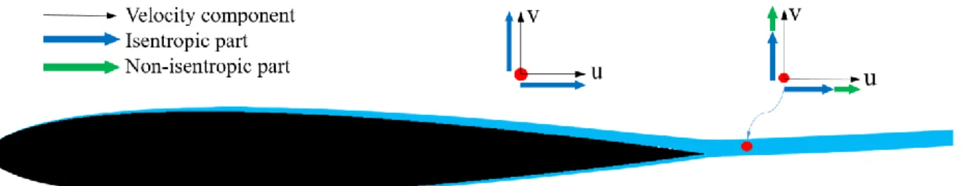
Nevertheless, the computation of the 𝛥𝑢∗ parameter relies on the measurement of the y- and z-velocity components, assuming an isentropic relation. This means that the Meheut’s decomposition assumes that the v and w velocities are isentropic in the entire domain (i.e., inside and outside the wake). This is true outside of the viscous wake of a body, where the flow is isentropic and then the u-, v- and w-components are truly isentropic. However, inside the wake and the boundary layer, all those three velocities have an isentropic and a non-isentropic component as shown in Fig. 2.

Fig. 2 Isentropic and non-isentropic parts of the velocity components.

Thus, using Eq. 6 to calculate the isentropic u-velocity from the real v- and w-velocities (that contains both, the isentropic and the non-isentropic components) is not exact and will lead to a small error. This error has shown to be negligible for far-field method applications. However, using this approach in the exergy equations lead to major errors. Thus a new velocity decomposition method suited for the exergy analysis is proposed as follows.

B. Proposed velocity decomposition method

The starting point is the isentropic relation used by Meheut [7]:

𝑃𝑠∗ 𝑃_𝑠0= [1 + 𝛾−1 2 𝑀0 2_{(1 −} 𝑢∗2+ 𝑣2+ 𝑤2 𝑢02 )] 𝛾 𝛾−1 (27)

Here, the v- and w-velocities contains both the isentropic and non-isentropic components. Thus, the same equation combines both, purely isentropic with non-isentropic components, which leads to an inaccuracy. However, this equations turns out to be exact if the isentropic velocity is used instead:

𝑃_𝑠∗ 𝑃_𝑠0 = [1 + 𝛾−1 2 𝑀0 2_{(1 −} 𝑉∗2 𝑢02)] 𝛾 𝛾−1 (28)

This equation simply relates the velocity magnitude with the static pressure in a fully isentropic field. It can be rewritten as: 𝑃_𝑠∗ 𝑃_𝑠0= [1 + 𝛾−1 2 𝑀0 2_{(1 −} 𝑢∗2+ 𝑣∗2+ 𝑤∗2 𝑢02 )] 𝛾 𝛾−1 (29)

Note that Eq. 29 is similar to Eq. 27 by the exception that the isentropic v- and w-velocities are now used. In fact, Meheut was only concerned with the isentropic u-velocity because his drag formulation (Eq. 2) only deals with this velocity component. This was well suited for far-field drag prediction but not for the exergy method.

Interestingly, Eq. 28 still holds for a real flow by acknowledging that:

𝑃𝑠≈ 𝑃𝑠∗ (30)

This means that the actual static pressure and the isentropic static pressure are practically equals in the entire domain. In other words, the static pressure field is not affected inside the viscous regions. This fact was demonstrated by Meheut and it will also be shown later in Figure 7. Hence, Eq. 28 can be rewritten as:

𝑃_𝑠 𝑃_𝑠0= [1 + 𝛾−1 2 𝑀0 2_{(1 −} 𝑉∗2 𝑢02)] 𝛾 𝛾−1 (31)

This enables expressing the isentropic velocity magnitude at each point of the domain as a direct function of the local static pressure, regardless of the region analyzed (i.e., isentropic or non-isentropic):

𝑉∗_{= 𝑢} 0√1 −_{(𝛾−1) 𝑀}2 02[( 𝑃𝑠 𝑃_𝑠0) (𝛾−1) 𝛾 − 1] (32)

Since the static pressure varies across the entire domain it will be more convenient to express the previous equation in terms of the total pressure because this parameter only changes inside the boundary layer and the wake of a body. The static pressure can be related to the total pressure by using isentropic relations [7]:

𝑃𝑠 𝑃_𝑠0= 𝑃_𝑡 𝑃_𝑡0∗ 𝜁 𝛾 (𝛾−1) (33) Where: 𝜁 = 1 +𝛾−1₂ 𝑀02(1 − 𝑉 2 𝑢02 𝑇_𝑡0 𝑇𝑡) (34)

Then, Eq. 32 becomes:

𝑉∗_{= 𝑢} 0√1 −_{(𝛾−1) 𝑀}2 02[( 𝑃_𝑡 𝑃_𝑡0) (𝛾−1) 𝛾 ∗𝜁− 1] (35)

This gives the isentropic velocity magnitude at any point of the domain as a function of the local total pressure, total temperature and real velocity (contained inside the ζ term).

In order to obtain the components of the isentropic velocity a major assumption will be made: the isentropic velocity vector is locally aligned with the real velocity vector. This assumption is based on the fact that the losses are convected by the flow, hence, the non-isentropic velocity vector will be aligned with the real velocity vector and consequently, the isentropic velocity vector will also be aligned. Thus, the direction cosines of the real velocity vector will be used to obtain the isentropic velocity components along the x-, y- and z-axes (See Fig. 3):

Fig. 3 Real velocity vector components.

{ 𝜃 = 𝑎𝑟𝑐𝑡𝑔( 𝑤 √𝑢2_+𝑣2) 𝛼 =𝑎𝑟𝑐𝑡𝑔 (𝑤_𝑢) 𝛽 =𝑎𝑟𝑐𝑡𝑔 (𝑣_𝑢) (36)

Then, the isentropic (inviscid) velocity components become:

𝑢∗_{= 𝑉}∗_{𝑐𝑜𝑠(𝜃) 𝑐𝑜𝑠(𝛽) (37)}

𝑣∗_{= 𝑉}∗_{𝑐𝑜𝑠(𝜃) 𝑠𝑖𝑛(𝛽) (38)}

𝑤∗_{= 𝑉}∗_{𝑠𝑖𝑛(𝜃) (39)}

Moreover, the non-isentropic (viscous) velocity components can be obtained by subtracting the isentropic velocity field from the real velocity field:

𝑢̅ = 𝑢 − 𝑢∗ ₍₄₀₎

𝑣̅ = 𝑣 − 𝑣∗ ₍₄₁₎

𝑤̅ = 𝑤 − 𝑤∗ ₍₄₂₎

IV.

Exergy breakdown method

The decomposition of the velocity field into its isentropic and non-isentropic components leads to the decomposition of the exergy terms into its isentropic and non-isentropic components. This exergy breakdown intends to highlights the physical origin of each type of exergy. “Isentropic exergy” stands for the exergy that is available at some point of the domain and that was created by a pure isentropic process (e.g., the velocity perturbation field outside the boundary layer). A “non-isentropic exergy” stands for the exergy available at some point of the domain and that was created by an entropy-generating process (e.g., the velocity deficit inside the boundary layer or wake).

The interest of decomposing each term of the exergy equation into its isentropic and non-isentropic part is related to the fact that the “isentropic exergy” is not useful from an engineering point of view for 2D cases because it represents a self-recovered exergy [15]: the perturbed flow outside the wake will follow an isentropic process downstream, thereby recovering all its related exergy potential once it reaches the equilibrium condition. On the other hand, the “non-isentropic exergy” represents the part of the exergy available inside an entropy-generating region. Hence, if this exergy is not recovered, it will be destroyed downstream by entropy-generating processes (e.g., turbulent mixing): it is up to the designer to recover that exergy before it becomes anergy. Hence, the exergy breakdown can provide a refined tool for practical design purposes. This concept will be further discussed in the next sections.

A. Mechanical exergy breakdown

The isentropic exergies are obtained by replacing their actual velocity components by the isentropic ones:

𝐸̇𝑢∗ = ∫_{𝑆𝑜𝑢𝑡}1₂𝜌(𝑢∗− 𝑢0)2 𝑢∗𝑑𝑆 (43)

𝐸̇𝑣∗= ∫_{𝑆𝑜𝑢𝑡}1₂𝜌(𝑣∗2+ 𝑤∗2) 𝑢∗𝑑𝑆 (44)

𝐸̇𝑝∗= ∫_{𝑆𝑜𝑢𝑡}(𝑃𝑠− 𝑃_𝑠0)( 𝑢∗− 𝑢0) 𝑑𝑆 (45)

As a reminder, a survey plane normal to the upstream flow direction is considered here (That’s why the V⃗⃗ . n⃗ term becomes u∗_{). On the other hand, the non-isentropic components are obtained by subtracting the isentropic field from}

the real field:

𝐸̇𝑢 ̅̅̅ = 𝐸̇𝑢− 𝐸̇𝑢∗ (46) 𝐸̇𝑣 ̅̅̅ = 𝐸̇𝑣− 𝐸̇𝑣∗ (47) 𝐸̇𝑝 ̅̅̅ = 𝐸̇_𝑝− 𝐸̇𝑝∗ (48)

The same decomposition also applies for the mechanical exergy:

𝜀̇

_̇

̇

̇

It is interesting to note that ε̇m and ε̇m∗ require an infinite surface integral on the entire survey plane, however ε̇̅̅̅̅ m

only requires a wake integral. This is because the difference of the real field and the isentropic field (i.e., ε̇m− ε̇m∗)

will provide the non-isentropic component (i.e., ε̇̅̅̅̅) that’s only related to the viscous and wave losses, thus, it is m

confined to the boundary layer, shockwave and wake region. Hence, a surface integral limited to the wake region is sufficient to compute ε̇̅̅̅̅ properly, simply because it has a null value at any point outside the boundary layer and m

wake zones (This is because ε̇̅̅̅̅ is a function of the non-isentropic velocity, that is limited to the wake region). The m

same reasoning also applies for its components: Ė̅̅̅u, 𝐸̇̅̅̅𝑣 and Ė̅̅̅p.

B. Thermal exergy breakdown

Thermal exergy also deals with velocity components, thus it admits a decomposition into its isentropic and non-isentropic parts. However, the thermal exergy also contains other parameters that are affected by the viscous effects

inside the boundary layer and the wake: the static temperature and density fields. Thus, they must be decomposed beforehand, by using the isentropic relations applied to the Eq.28 as follows:

𝑇𝑠∗= 𝑇_𝑠0[1 +𝛾−1₂ 𝑀02(1 − 𝑉 ∗2 𝑢02)] (51) 𝜌∗_{= 𝜌} 0[1 +𝛾−1₂ 𝑀02(1 − 𝑉 ∗2 𝑢₀2)] 1 𝛾−1 (52)

Then, by using Eq. 51 and 52, and considering a survey plane perpendicular to the upstream flow direction (i.e.,V⃗⃗ . n⃗ = 𝑢), the isentropic thermal exergy (Eq. 15) becomes:

𝜀̇

_𝜀̇

𝜀̇

𝜀̇

∫

[1 −

(

)]

∫

𝜀̇

∫

[1 −

(

)]

∫

Finally, the non-isentropic thermal exergy is given by subtracting the isentropic part from the total field:

𝜀̇𝑡ℎ

̅̅̅̅ = 𝜀̇𝑡ℎ− 𝜀̇𝑡ℎ∗ (56)

As it was explained before, the integral of the non-isentropic thermal exergy is also reduced to the wake region.

C. Exergy-based drag breakdown

According to the Arntz proposition (Eq. 24), the drag field distribution at a given survey plane position is a combination of the exergy and anergy fields. Since the exergy-based drag is a function of the exergy, and in turn, the exergy can be broken down into its isentropic and non-isentropic parts, we can extend this concept in order to decompose the exergy-based drag field into its isentropic and non-isentropic parts as follows:

𝐶_𝐷𝜀∗ ₌ 𝜀̇𝑚∗+𝜀̇𝑡ℎ∗ 1

2𝜌0 𝑢03 𝑆𝑟𝑒𝑓

(57)

𝐶𝐷̅̅̅̅ _𝜀 = 𝐶_𝐷𝜀− 𝐶_𝐷𝜀∗ (58)

Again, the objective of this breakdown is to highlight the physical origin of the drag components at a given survey plane position. “Isentropic drag” stands for the part of the drag field distribution linked to perturbations of isentropic origin (e.g., the velocity perturbation outside the boundary layer or wake). On the other hand,

“non-isentropic drag” is the part of the drag field distribution linked to perturbations created by entropy-generating mechanisms (e.g., the velocity deficit inside the boundary layer or wake). Of course, this is plane-dependent in the sense that a particle could have followed a purely isentropic process up to certain plane position but maybe downstream this particle penetrates the wake. At that point, the particle will contain both, isentropic and non-isentropic perturbations.

Note that the isentropic drag coefficient C_Dε∗ does not include the anergy term as it does in the total drag coefficient equation (Eq.24). This is because the anergy takes into account the losses and it must not be considered for the isentropic drag component. Nevertheless, anergy is implicitly present in Eq.58 across the C_Dε term, thus, the anergy is included into the non-isentropic drag coefficient.

On the other hand, C_Dε and C_Dε∗ _{must be integrated on the entire survey plane since these fields varies across the}

entire domain. However, CD̅̅̅̅ ε only requires a wake integral because its field is zero outside the wake region:

∫_𝑆 𝐶_𝐷𝜀 𝑑𝑆

𝑜𝑢𝑡 = ∫ 𝐶𝐷𝜀

∗ _𝑑𝑆

𝑆_𝑜𝑢𝑡 + ∫ 𝐶𝑆_𝑤 𝐷̅̅̅̅ 𝜀 𝑑𝑆 (59)

For 2D cases, the integral of the non-isentropic exergy drag coefficient CD̅̅̅̅ ε will provide the profile drag. Moreover, the integral of the isentropic component is negligible, as it will be shown later in Figure 26:

𝐹𝑜𝑟 2𝐷 𝑐𝑎𝑠𝑒𝑠: ∫_𝑆 𝐶_𝐷𝜀 𝑑𝑆

𝑜𝑢𝑡 = ∫ 𝐶𝐷𝜀

∗ _𝑑𝑆

𝑆𝑜𝑢𝑡 + ∫ 𝐶𝑆𝑤 𝐷̅̅̅̅ 𝜀 𝑑𝑆= 0 + 𝑝𝑟𝑜𝑓𝑖𝑙𝑒 𝑑𝑟𝑎𝑔 (60)

For 3D cases, C_{D̅̅̅̅ ε} will also provide the profile drag. The induced drag is automatically transferred to the isentropic component 𝐶_𝐷𝜀∗ when the velocity decomposition is used. Hence, the total drag becomes:

𝐹𝑜𝑟 3𝐷 𝑐𝑎𝑠𝑒𝑠: ∫_𝑆 𝐶_𝐷𝜀 𝑑𝑆

𝑜𝑢𝑡 = ∫ 𝐶𝐷𝜀

∗ _𝑑𝑆

𝑆𝑜𝑢𝑡 + ∫ 𝐶𝑆𝑤 𝐷̅̅̅̅ 𝜀 𝑑𝑆= 𝑖𝑛𝑑𝑢𝑐𝑒𝑑 𝑑𝑟𝑎𝑔 + 𝑝𝑟𝑜𝑓𝑖𝑙𝑒 𝑑𝑟𝑎𝑔 (61) This mathematical behavior is not surprising because the same happened with the far-field formulations [7] where the momentum conservation equation provided the total drag, whereas the Meheut’s method (that uses the velocity decomposition) only provided the profile drag for 2D and 3D cases. In fact, the transverse flow associated with the wingtip vortices is purely isentropic outside the wake, thus, it is already included in the C_Dε∗ term through the ε̇m∗ component. This explains why CD̅̅̅̅ ε does not contain the induced drag. However, this transverse flow is linked to the axial vorticity field left downstream by the body inside its wake [16], which is accounted for separately

by the Ėv wake method (Eq.18). Thus, in the far-field and exergy methods with velocity decomposition, the induced

drag (transverse exergy) must be added to the profile drag (non-isentropic exergy drag). This will be explained in detail in the next sections.

V.

CFD data

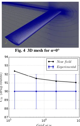
2D and 3D CFD data will be used for the analysis of the velocity decomposition method and the new exergy formulations. The 2D case is a NACA 0012 airfoil with a sharp trailing edge. The 3D case is a rectangular wing of aspect ratio 8 with the same airfoil and a rounded wing tip. In both cases a C-block structured grid with wake refinement was used (See Fig. 4). The domain extent is 150 chords in all directions for the 2D case and 30 chords for the 3D case. For the 2D case, a grid refinement was performed and the near-field drag value compared against experimental data of the bibliography [24-27] as shown in Fig.5. Then the mesh of 593,000 cells was selected for the 2D case, which ensured the correct capture of all the physical phenomena even in transonic conditions. For the 3D case, a similar 2D mesh was extruded spanwise resulting in a mesh of 9.2 million cells. The mesh blocking and refinement on the wake region was different for each angle of attack for both 2D and 3D meshes: the refinement zone follows the wake deviation in order to ensure a proper capture of the wake.

Fig. 4 3D mesh for α=0°

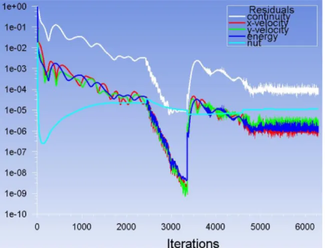
The 2D and 3D cases were analyzed for several angles of attack at a constant Mach number of 0.3 and 0.8, at a Reynolds number of 3x106. In all the cases, RANS simulations were performed with the Spalart Allmaras turbulence model. A first quick convergence was done with a first-order discretization (flow and turbulence) by about 3000 iterations, followed by a final second-order discretization convergence as shown in Fig. 6. All the simulations were left running until the near-field drag coefficient residual was less than 0.1 drag counts. At the same time, the residuals must reach their maximum precision in order to ensure that the airfoil’s losses were completely transmitted (convected) downstream. Then, the y+ parameter was controlled in order to verify that y+≤1 everywhere around the body (as required by the Spalart Allmaras model). The resulting CFD data was analyzed with a Paraview plugin called Epsilon [19], an Open Source code developed by ISAE-SUPAERO which performs far-field and exergetic analyses.

Fig. 6 Residuals convergence for the airfoil at α=0°/M=0.3

VI.

Velocity decomposition analysis

In this section, different flow field parameters are analyzed in order to highlight the facts already mentioned during the development of the formulation.

A. Static pressure field

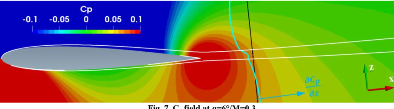
The starting point of the velocity decomposition procedure was the acknowledgement that the static pressure field is practically not affected inside the boundary layer and wake regions as it was proven by Meheut [7]. This has led to the assumption that the isentropic static pressure is actually the real static pressure (i.e., P_s≈ P_s∗). This is observed in Fig. 7, where the pressure coefficient field is shown around a NACA 0012 airfoil, along with a white line that delimits the boundary layer and wake region. The field outside these lines is isentropic and the field inside

is non-isentropic. It can be clearly seen that the Cp field does not suffer a distortion inside the non-isentropic region. Instead, the Cp contour lines cross the viscous region without suffering a noticeable kink in those lines. In order to highlight this fact, Fig.7 also shows the distribution of the Cp gradient along a black survey line (placed normal to the upstream flow direction). The Cp gradient is a parameter very sensitive to the distortions. However, it is observed that the degree of distortion suffered by this gradient distribution is quite small inside the viscous region.

Fig. 7 Cp field at α=6°/M=0.3

Any kink of the contour lines would be a clear trace of the presence of a non-isentropic region. This can be observed in Fig. 8 for the w-velocity field, where the contour lines are deformed across the wake because of the presence of a non-isentropic region (purely viscous effect in this case). Hence, it can be concluded that the pressure field is practically not affected by the viscous phenomena because their contour lines are not kinked, hence, Ps≈

Ps∗.

Fig. 8 w-velocity field at α=6°/M=0.3 B. Meheut’s velocity decomposition applied to the exergy method

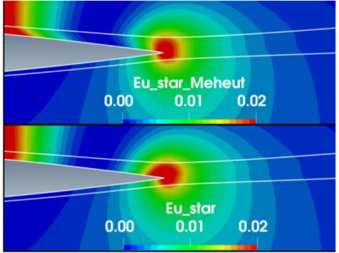
If the velocity decomposition proposed by Meheut is used for the breakdown of the exergy equations, it does not succeed in taking away the kink (distortion) from the contour lines across the non-isentropic region. This can be observed for the isentropic axial exergy field 𝐸̇𝑢∗ in Fig. 9, where a large kink is observed across the viscous region

(see upper left of upper image). Instead, the new method (lower image) provides a smoother field than the Meheut’s method. The kink of the contour line for the Meheut’s method is even worse for Ėv∗ because the transverse velocities

kink of the Meheut’s method did not compromise the accuracy in far-field method applications. Nevertheless, these distortions shown to be excessive for the exergy method. In fact, the Meheut profile drag equation (Eq. 2) only deals with the square of the velocity components, whereas the exergy terms (Eq. 43, 44 and 49) deal with the cubic law of the velocity components. Hence, any distortion of the contours of the velocity components across the non-isentropic region will be amplified by the exergy equations leading to unacceptable errors.

Fig. 9 𝐄̇𝐮∗ field at α=6°/M=0.3

C. New velocity decomposition

The new velocity decomposition formulation enables extracting the isentropic part “u∗_{” and the non-isentropic}

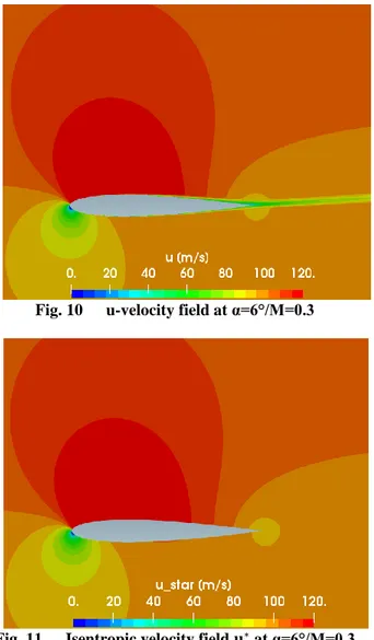
part “u̅” from the velocity field “u”. This is shown in Fig. 10, where the actual velocity field is shown as the starting point. Then in Fig. 11, only the isentropic part is retained, i.e., the effect of the viscous losses on the velocity field is taken away leaving a pure inviscid flow field. Note that this field is equivalent to the potential flow around the airfoil [17]. On the other hand, Fig. 12 shows the non-isentropic part that has been extracted, i.e., it only contains the viscous effect on the velocity field. Since the boundary layer and the wake create losses, and those losses are observed as a velocity deficit, the non-isentropic velocity field is negative inside the viscous region. This velocity deficit is due to the loss of momentum inside the viscous region, associated with the drag (momentum transfer from the fluid to the body). Also note that this non-isentropic velocity is null outside the boundary layer and wake region. That’s why its integral can be reduced to the wake region only.

Fig. 10 u-velocity field at α=6°/M=0.3

Fig. 11 Isentropic velocity field 𝐮∗ at α=6°/M=0.3

Fig. 12 Non-isentropic velocity field 𝐮̅ at α=6°/M=0.3

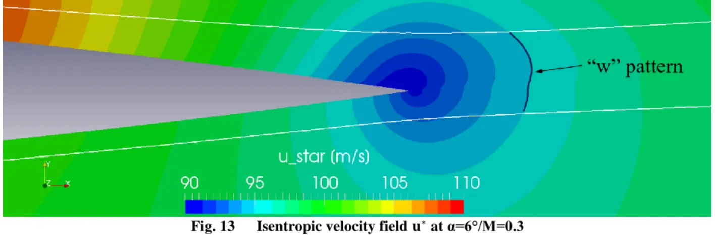
In order to analyze the decomposition capabilities of the proposed method, a close up is made around the trailing edge region for the isentropic u- and w-velocity fields (Figs. 13 and 14 respectively). The u∗ field shows a very small kink across the boundary layer limit and a w-like kink pattern across the wake region. Nevertheless, this kink is very small.

Fig. 13 Isentropic velocity field 𝐮∗ at α=6°/M=0.3

On the other hand, the w∗ velocity field shows an s-like kink pattern across the wake. This oscillation is developed around the mean contour line inside the wake region. It can be seen that the deviations from the mean line are not small but it has not shown to have a negative impact on the exergy decomposition. In fact, the positive and negative oscillation (around the mean line) of the contour lines inside the wake seems to be self-compensated during the integration (This is a matter of further study). Moreover, the fact of decomposing the transverse velocities represents a significant advantage over the Meheut’s method where the “v” and “w” velocities are not decomposed at all.

Fig. 14 Isentropic velocity field 𝐰∗ at α=6°/M=0.3

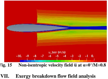
It is important to highlight that the non-isentropic velocity field is related not only to the viscous losses but also to the wave losses. This can be clearly seen in Fig. 15 where a velocity deficit is also observed across the shock wave region.

Fig. 15 Non-isentropic velocity field 𝐮̅ at α=0°/M=0.8

VII.

Exergy breakdown flow field analysis

In this section an analysis of the different decomposed exergy parameters will be made in order to highlight the facts already mentioned during the development of the formulation. This will be performed with 2D and 3D data, for subsonic and transonic conditions as well.

A. 2D subsonic

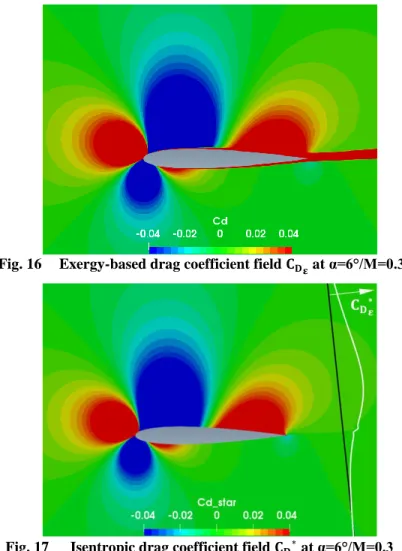
The velocity decomposition applied to the exergy formulation enables obtaining its isentropic and non-isentropic components. This is shown for the case of the exergy-based drag coefficient in Fig. 16, 17 and 18. Here is reminded that the breakdown of any parameter into its isentropic and non-isentropic components intends to highlight the physical origin of each component: the isentropic part is related to isentropic perturbations whereas the non-isentropic part is related to perturbations created by entropy-generating mechanisms. Note that the non-isentropic component C_Dε∗ takes away the influence of the losses that occur inside the boundary layer and the wake. It only retains the part of the field associated with an isentropic evolution (equivalent to a potential flow [17]). Also note that this field varies at every point of the domain: a survey plane placed downstream of the airfoil (black line) will detect non-zero values of this field along it (white curve). However, when these values are integrated along the line, the result is a zero net contribution to the drag coefficient in 2D cases (it will be shown numerically later in Figure 26). This confirms the fact that the isentropic exergy field is not interesting for design purposes in 2D cases [15] because the related exergy is self-recovered downstream since the flow particles follow an isentropic trajectory; they return to the original (equilibrium) state by following a reversible path. This highlights the need of decomposing the exergy formulations in order to retain only the interesting part of the exergy from a design point of view: the non-isentropic field.

Fig. 16 Exergy-based drag coefficient field 𝐂_𝐃𝛆 at α=6°/M=0.3

Fig. 17 Isentropic drag coefficient field 𝐂_𝐃𝛆∗ at α=6°/M=0.3

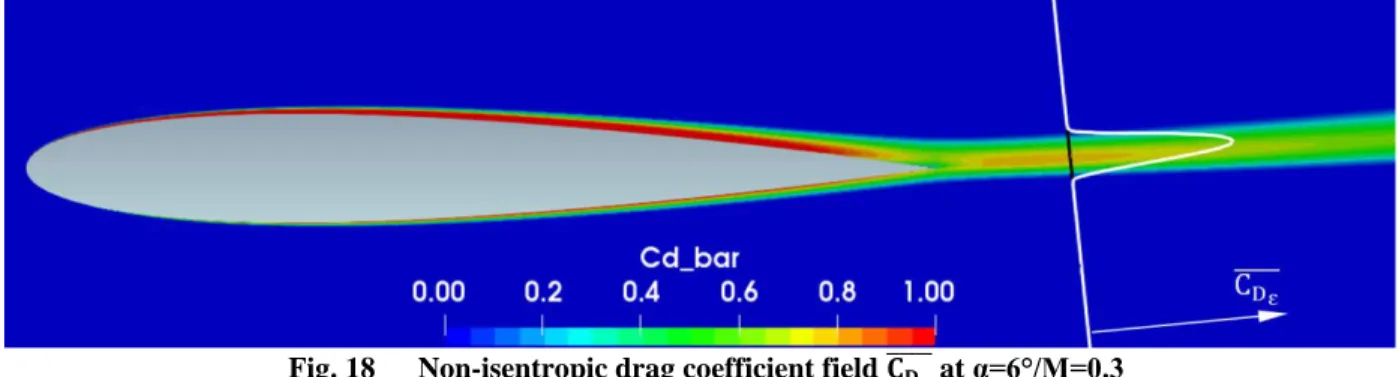
The non-isentropic exergy-based drag coefficient field (related to viscous and shockwave losses) is shown in Fig. 18. This field is zero outside the boundary layer and the wake as expected since no entropy-generating mechanism exists there. This can be best observed by the help of the black survey line placed normal to the upstream flow direction and along which the CD̅̅̅̅ _ε distribution is shown. The integral of this distribution (Eq. 58) will provide the profile drag coefficient, and since this field is null outside the wake, the related integral is reduced to the wake region. This demonstrates that the decomposed exergy formulation is suited for wind tunnel data analysis, whereas the original Arntz’s method requires an infinite survey plane integral since it also integrates the isentropic components (whose field varies at any point of the domain). Moreover, the CD̅̅̅̅ _ε distribution along the survey line matches the distribution of C_Dε (not shown here for simplicity), thus, it will also differ from the Meheut’s profile drag distribution [15].

Fig. 18 Non-isentropic drag coefficient field 𝐂̅̅̅̅̅ at α=6°/M=0.3 _𝐃𝛆

In order to assess the effectiveness of the velocity decomposition for the exergy formulation, the isentropic drag field close to the trailing edge region is analyzed in Fig. 19. It can be observed that the contour lines only present a very weak kink across the wake region for small angles of attack. For larger angles of attack (Fig. 20) the kink increases but it adopts an s-like pattern that is self-compensated during the integration.

The conclusions from the analysis of the isentropic and non-isentropic exergy drag fields also applies to its components (Mechanical exergy, thermal exergy and so on), thus it is not shown here for simplicity.

Fig. 19 Isentropic drag coefficient field 𝐂_𝐃𝛆∗ at α=0°/M=0.3

B. 2D transonic

In transonic conditions, the non-isentropic exergy-based drag coefficient field also highlights the wave losses as shown in Fig. 21 (because the shockwave it is also an entropy-generating mechanism). Its related distribution along the black survey line is also shown, where the wave drag corresponds to the part of the distribution lying on the top of the green region. This wave drag can be extracted from the CD̅̅̅̅ _ε distribution by using the method previously proposed by the authors [14], suited for wind tunnel testing.

Fig. 21 Non-isentropic drag coefficient field 𝐂̅̅̅̅̅ at α=0°/M=0.8 _𝐃𝛆 C. 3D subsonic

In order to analyze the impact of the velocity decomposition method on the exergy equations, a survey plane will be placed at one chord downstream of the wing, normal to the upstream flow direction (Fig. 22). Then, the distributions of the components of the exergy-based drag coefficient are shown in Fig. 23. It clearly depicts that the isentropic component (Fig. 23b) takes away the viscous effects, retaining only the inviscid component. Instead, the non-isentropic component (Fig. 23c) only retains the losses and its related field is null outside the wake. Its integral will provide the profile drag but not the total drag of the body. As it was explained before, the implementation of the velocity decomposition to the exergy equation will retain only the profile drag in the non-isentropic term but not the induced drag. Indeed, the induced drag is transferred to the isentropic field as it will be demonstrated later in Figures 33 and 35. This means that the isentropic exergy-based drag coefficient field shown in Fig. 23b is mostly induced drag and its field varies on the entire survey plane. However, this transverse flow is linked to the axial vorticity field shed by the body. Thus, the induced drag can be expressed as a function of wake parameters and integrated on the wake only (Eq. 18) as it has been previously proved by the authors [16].

Fig. 22 Wing and survey plane at α=10°/M=0.3

Fig. 23 Exergy-based total drag (a), induced drag (b) and profile drag (c) D. 3D transonic

In the transonic regime the observations are similar to the subsonic case as shown in Fig. 24 and 25. The difference here is that the non-isentropic exergy-based drag coefficient (profile drag) also contains the losses associated with the shockwave. The shockwave volume is colored in violet in Fig. 24 and its wake is the green region in Fig. 25c. The wave drag can thus be extracted from this field by using the technique previously proposed by the authors [14]. Note that the angle of attack in this transonic case is smaller than the subsonic case presented before: that is why the intensities of the induced and profile drag distributions are weaker.

Fig. 24 Wing and survey plane at α=3°/M=0.75

Fig. 25 Exergy-based total drag (a), induced drag (b) and profile drag (c)

VIII.

Exergy breakdown data analysis

In this last section, a numerical analysis of the velocity decomposition is performed for several angles of attack. Hereafter, the survey plane used will be placed at one chord downstream of the body because it is the typical survey plane position used in wind tunnel testing and also because the proposed formulation is intended to be used for wind tunnel data analysis only (although its application for CFD posttreatment is also useful for design purposes). However, it must be acknowledged that for this survey plane position the available exergy is not at a maximum [13, 14] but it will be useful to present some new concepts.

The breakdown of the exergy-based drag coefficient (Eq. 58) is shown in Fig. 26. It can be seen that the non-isentropic drag 𝐶_{𝐷̅̅̅̅ 𝜀} (whose integral is reduced to the wake) matches the exergy drag curve C_Dε (that requires an infinite surface integral). This highlights the usefulness of the velocity decomposition: the Arntz equations are now reduced to the wake and a proper exergy analysis can be made with wake data from wind tunnel testing.

On the other hand, the isentropic drag coefficient C_Dε∗ is zero or negligible in the entire range of angle of attack studied. This proves that this component does not contribute to the drag of a body (in 2D cases) even though its field is non-zero on the entire survey plane. Indeed, the related perturbations follow a reversible transformation downstream, thus, its exergy is self-recovered and its integral is zero. It is worth mentioning that this term has been integrated on the entire survey plane (The only parameters that can be integrated in the wake region are the non-isentropic exergies).

Fig. 26 Exergy drag coefficient breakdown (2D-NACA0012-M=0.3-Re=3x106)

In order to show the accuracy of the new exergy method reduced to the wake, a comparison against other methods is presented in Table 1, where far-field values (Meheut’s method) had required a wake integral and the Arntz method required an infinite surface integral.

Table 1 profile drag coefficient values (drag counts)

α (°) Near-field Far-field Exergy Arntz Exergy wake Wake - Arntz

0 91.58 91.12 91.80 91.35 -0.45 2 93.41 92.74 93.51 93.05 -0.46 4 99.08 98.14 98.03 97.60 -0.43 6 109.45 108.06 106.76 106.42 -0.34 8 126.2 124.31 125.48 123.89 -1.59 10 154.07 151.53 153.97 151.90 -2.07

Note that a very good agreement is observed: the scatter between the Arntz and the wake methods lies in the ±2dc range. This is within the typical experimental uncertainty for drag prediction [25]. Also note the very good agreement between both wake-reduced methods: far-field and exergy. Both formulations provides the profile drag with the same order of accuracy, however, exergy analysis is even more powerful since it admits a further profile drag breakdown: the exergy-based characteristic curves.

The exergy-based characteristic curves [14] are shown in Fig. 27. This decomposes the non-isentropic drag coefficient CD̅̅̅̅ _ε (profile drag) into its exergy and anergy components. The difference between the non-isentropic drag and the anergy curve (CD̅̅̅̅ _ε − C𝒜̇ ) represents the total exergy, i.e., the maximum theoretical amount of power

that can be recovered (drag reduction possibilities). Since the thermal exergy C_{ε̇̅̅̅̅̅ th} is negligible for external aerodynamic cases without heat transfer, this total available exergy is mainly given by the mechanical exergy Cε̇̅̅̅̅ m . As a reminder, the survey plane was taken one chord downstream of the body, that’s why the available exergy is not that much (it is maximum at the trailing edge of the body). However, this breakdown is one of the major assets of the new method since it provides the profile drag as well as its exergy and anergy components: the physical analysis is more in-depth with the new exergy approach, leading to better design opportunities. Moreover, if closer survey plane positions are required (associated with higher exergy availability), a modified wake exergy technique must be used [17].

Fig. 27 Exergy characteristic curves (2D-NACA0012)

The previous exergy characteristic curves can be complemented by another breakdown of the isentropic and non-isentropic exergy terms (Figures 28 and 29 respectively). The breakdown of the non-isentropic terms shows that the

isentropic mechanical exergy Cε̇_m∗ is almost zero for 2D cases regardless the angle of attack, meaning that no net energy can be recovered from this isentropic field regardless the fact that CĖu∗, CĖv∗ and CĖp∗ are non-zero. As a matter

of fact, those terms are linked by the pressure-velocity coupling mechanisms: CĖ_p∗ compensates the existence of isentropic kinetic exergy (CĖu∗+ CĖv∗), leading to a net zero mechanical exergy. Also note that Cε̇th∗ is negligible. This highlights the fact that the 2D isentropic field around a body does not contain any drag-generating mechanism (there is no net energy to be wasted downstream by entropy-generating mechanisms).

Fig. 28 Breakdown of isentropic components (2D-NACA0012)

The non-isentropic components are related to viscous/shockwave phenomena, hence related to a drag generation. This drag in given by the mechanical exergy (as well as the anergy – not shown here-) and that is why the Cε̇̅̅̅̅_m curve is positive. This net mechanical exergy C̅̅̅̅ε̇m is composed by the CĖ̅̅̅̅u, CĖ̅̅̅̅v and CĖ̅̅̅̅p fields, with CĖ̅̅̅̅v being a

small quantity in 2D cases. Note that the airfoil creates a certain amount of axial kinetic exergy C_Ė u

̅̅̅̅ related to the axial velocity deficit in the viscous region, however, not all this exergy is potentially recoverable. In fact, part of C_Ė̅̅̅̅_u

has been generated at the expense of C_Ė p

̅̅̅̅. That is why C_ε̇̅̅̅̅_m is the parameter that quantifies the net recoverable amount of energy. Hence, the interest of this breakdown is to pinpoint the flow topology and to get an initial guess about the type of energy recovery system to be used. In this case, a BLI system is well suited to recover Cε̇̅̅̅̅_m, that’s

Fig. 29 Breakdown of non-isentropic components (2D-NACA0012)

All the curves in this study corresponds to a survey plane position of one chord downstream of the body. The effect of moving downstream the survey plane is shown in Fig 30 and 31. It can be seen that 𝐶𝐷̅̅̅̅ _𝜀 provides the same value regardless the survey plane position. Also, the anergy C𝒜̇ increases as the survey plane moves downstream due

to the exergy destruction process (mainly by viscous dissipation along the wake). This demonstrates that the exergy is a maximum at the trailing edge of the body: hence a BLI system must be placed closer to the airfoil trailing edge in order to recover a maximum amount of energy.

Fig. 31 shows a breakdown of this net exergy Cε̇̅̅̅̅m, confirming again that the total exergy is mainly given by CĖ̅̅̅̅_u

(related to the velocity deficit inside the wake) for 2D cases. The pressure effect C_Ė p

̅̅̅̅ is only present for closer survey plane positions due to the potential effect of the body.

Fig. 31 Survey plane sweep downstream: breakdown (2D-NACA0012)

The power recovery principle associated with the exergy method also leads to the introduction of a new concept: the exergy-based lift-to-drag ratio “(L/D)ε“ as shown in Fig. 32. In fact, the classical lift-to-drag ratio “L/D” takes into account the profile drag for its calculation. However, since the total exergy available at the survey plane is theoretically recoverable, this profile drag could be reduced to the total anergy only, i.e., D=𝒜̇ and the lift-to-drag ratio becomes L/𝒜̇ or simply “(L/D)ε“ in order to emphasize the fact that this is achieved by recovering the exergy. The exergy-based lift-to-drag ratio stablishes the upper theoretical limit for the lift-to-drag ratio curve. This means that the actual L/D of a body can be improved by recovering its exergy downstream, and if all the exergy is recovered, L/D reaches (L/D)ε: it is physically impossible (for a given geometry, flight condition and survey plane) to overtake this limit. This parameter is very useful for design purposes because it provides a metric to know if it’s worth investing a design effort to deploy energy recovery devices, depending on the remaining margin to be recovered. Here it is reminded that the available exergy is at a maximum when the survey plane is closer to the body. For that plane position, the (L/D)ε curve will have higher values than that of Fig. 32.

Fig. 32 Exergy-based lift-to-drag ratio (2D-NACA0012) B. 3D subsonic case

The results of the breakdown of the exergy formulation for a 3D case, the NACA0012 wing, are shown in Fig. 33. The exergy-based drag coefficient C_Dε (Eq. 24) is splitted into its isentropic C_Dε∗ (Eq. 57) and non-isentropic 𝐶𝐷̅̅̅̅ _𝜀

(Eq. 58) components. Here is reminded again that this breakdown highlights the physical origin of each component: the isentropic part is related to isentropic perturbations whereas the non-isentropic part is related to perturbations created by entropy-generating mechanisms. Both type of perturbations are linked to drag generation for 3D cases.

First of all, it must be noticed that the non-isentropic drag 𝐶𝐷̅̅̅̅ 𝜀 provides the profile drag since it is related to the viscous and shockwave losses (entropy generating mechanisms). As a matter of fact, the 𝐶𝐷̅̅̅̅ 𝜀 distribution matches the Meheut’s profile drag curve 𝐶𝐷_{𝑝 𝑀𝑒ℎ𝑒𝑢𝑡}. Here is also worth mentioning that both the 𝐶𝐷̅̅̅̅ _𝜀 and the Meheut’s profile

drag formulations have been integrated in the wake region only (both formulations are well suited for wind tunnel testing).

Secondly, the isentropic curve C_Dε∗ _{provides the induced drag, since this is the drag associated to the transverse}

rotational flow field created by the wing, which is of isentropic origin (this rotational flow field lies mainly in the isentropic region of the flow). Note that C_Dε∗ matches the wake’s transverse exergy curve 𝐶𝐸_{𝑣 𝑤𝑎𝑘𝑒} (Eq. 18). This

means that both formulations provide the induced drag but from different points of view: C_Dε∗ requires an infinite survey plane integral whereas 𝐶𝐸𝑣 𝑤𝑎𝑘𝑒 only requires a wake integral. Hence, in practice (wind tunnel testing), the induced drag will be determined only by the 𝐶𝐸_{𝑣 𝑤𝑎𝑘𝑒} method.

Fig. 33 Drag breakdown (3D-NACA0012 wing-M=0.3-Re=3x106)

Finally, when the 𝐶𝐷̅̅̅̅ 𝜀 (profile drag) is added up to 𝐶𝐸𝑣 𝑤𝑎𝑘𝑒 (induced drag), the total drag can be retrieved; this total drag curve matches with the C_Dε curve. In fact, C_Dε is the total drag of a body given by the Arntz’s formulation, which requires an infinite survey plane integral. Instead, the sum “𝐶𝐷̅̅̅̅ 𝜀 + 𝐶𝐸𝑣 𝑤𝑎𝑘𝑒” only requires a wake integral. This can be summarized as follows:

𝐹𝑜𝑟 3𝐷 𝑐𝑎𝑠𝑒𝑠: 𝐶_{𝐷𝑡𝑜𝑡𝑎𝑙} = 𝐶_{𝐷𝑝𝑟𝑜𝑓𝑖𝑙𝑒}+ 𝐶_{𝐷𝑖𝑛𝑑𝑢𝑐𝑒𝑑}= ∫ 𝐶𝑆𝑤 𝐷̅̅̅̅ 𝜀 𝑑𝑆+ ∫

1 2𝜌 𝜓 𝜉 𝑢

∗ _𝑑𝑆

𝑆𝑤 (62)

This demonstrates that all the exergy parameters can be computed from wake data only, leading to a formulation suited for wind tunnel testing. Also note that C_Dε∗ is not an interesting parameter for wind tunnel applications because it has been replaced by 𝐶𝐸_{𝑣 𝑤𝑎𝑘𝑒} (A more practical parameter).

On the other hand, the fact that the integral of the isentropic exergy-based drag C_Dε∗ _{is zero in 2D but non-zero in}

3D (and equal to the induced drag) can be misleading. However, since induced drag is zero for 2D cases, it is reasonable to find a zero value for the integral of C_Dε∗ _{in 2D cases.}

The accuracy of this new method is compared against other methods in Table 2, where the new “Exergy wake” method is given by the Eq. 62. A good agreement is observed up to α=10°, but the error increases for larger angles of attack. In order to understand the source of this error, Table 3 shows the breakdown of the total drag into its profile and induced drag, where the Meheut method is taken as a reference. It can be observed that the profile drag given by 𝐶𝐷̅̅̅̅ _𝜀 provides accurate values up to 10° followed by a small under prediction for larger angles of attack (but the related error is acceptable). However, it can be observed that the major source of error comes from the induced

drag given by ∫ 1

2𝜌 𝜓 𝜉 𝑢 ∗ _𝑑𝑆

𝑆_𝑤 . This expression only provides an approximation of the true induced drag given by

C_Dε∗ _.

Table 2 total drag coefficient (drag counts)

α (°) Near-field Far-field Exergy Arntz Exergy Wake Wake-Arntz [%]

0 94.61 93.20 95.68 93.64 -2.12 2 110.58 107.08 108.94 106.82 -1.95 4 149.43 145.12 147.65 145.46 -1.54 6 213.66 210.97 212.91 211.96 -0.57 8 304.08 300.94 303.73 307.09 0.89 10 420.28 417.60 421.44 432.94 2.43 12 563.69 561.95 563.75 588.99 4.48 14 736.95 735.47 736.08 779.55 5.78

Table 3 comparison of wake formulations (drag counts)

α (°) Far-field Exergy Wake

Profile drag New-Meheut [%] Induced drag New-Meheut [%] Profile Induced Total Profile Induced Total

0 93.20 0.00 93.20 93.64 0.00 93.64 0.47 -0.60 2 95.74 11.34 107.08 95.51 11.30 106.82 -0.24 -0.35 4 99.68 45.44 145.12 99.67 45.79 145.46 -0.01 0.77 6 109.37 101.59 210.97 107.98 103.98 211.96 -1.27 2.35 8 121.55 179.39 300.94 119.99 187.10 307.09 -1.28 4.30 10 142.11 275.48 417.60 140.22 292.72 432.94 -1.34 6.26 12 173.23 388.71 561.95 167.32 421.67 588.99 -3.42 8.48 14 230.96 504.51 735.47 222.29 557.26 779.55 -3.75 10.46

The advantage of the exergy method over the far-field method is that total drag 𝐶_{𝐷𝑡𝑜𝑡𝑎𝑙} can be decomposed into its exergy and anergy components (exergy characteristic curves) as shown in Fig. 34. The difference between the total drag (𝐶𝐷̅̅̅̅ 𝜀 + 𝐶𝐸𝑣 𝑤𝑎𝑘𝑒) and the anergy C𝒜̇ gives the total exergy (Predominated by the total mechanical exergy since in an adiabatic subsonic case, the thermal exergy 𝐶ε̇̅̅̅̅̅ 𝑡ℎ is negligible). For 3D cases, the total mechanical exergy is given by 𝐶_{̅̅̅̅ ε̇𝑚}+C_εm∗ , and represents the total amount of energy that could be theoretically recovered by a device placed downstream of the body. Note that this mechanical exergy is mostly composed by the transverse exergy 𝐶𝐸_{𝑣 𝑤𝑎𝑘𝑒} (the axial and pressure exergies are very small in this case).

Fig. 34 Exergy characteristic curves (3D NACA0012 wing)

The breakdown of the isentropic components of C_Dε∗ _{will shed more light on the previous analysis as shown in}

Fig. 35. In fact, C_εm∗ was zero for 2D cases (see Fig. 28) but not for 3D flows. In fact, for 2D flows CĖu∗ and CĖv∗ are compensated by CĖ_p∗ leading to a zero net mechanical exergy. In 3D flows this physical behavior is still present but

coexists with an additional isentropic phenomena: the transverse rotational flow related to the lift. Since this rotational flow field is not concentrated in the wake region, it is not of viscous nature, thus isentropic (although it can be related to the wake information, through the axial vorticity, thanks to the 𝐸𝑣 𝑤𝑎𝑘𝑒 formulation). This explains

why C_εm∗ is not zero in 3D flows. Moreover, since C_Ėv∗ is linked to the axial vorticity field, and this vorticity is dissipated downstream by entropy-generating mechanisms, it is clear that C_Ėv∗ will also decrease downstream (exergy destruction into anergy).

The breakdown of the non-isentropic components of 𝐶𝐷̅̅̅̅ _𝜀 is shown in Fig. 36. The difference of this figure

compared to the 2D case (Fig. 29) is that the existence of the wing-tip vortex creates an additional pressure-velocity phenomena associated to the low pressure at the vortex core. Since the axial vorticity increases with the angle of attack, this pressure-velocity coupling is expected to increase as well.

Fig. 36 Breakdown of non-isentropic components (3D NACA0012 wing)

Finally, the exergy recovery principle leads to the definition of the exergy-based lift-to-drag ratio as shown in Fig. 37. This curve shows that a significant potential for power recovery is available for 3D cases. The difference between the L/D and (L/D)ε curves is mainly driven by 𝐶𝐸_𝑣 (when the survey plane is placed at one chord

downstream of the body).

IX.

Conclusion

A new velocity decomposition method based on the Meheut’s approach was developed in order to decompose the Arntz’s exergy formulations. This allowed obtaining the isentropic and the non-isentropic parts of the exergy (associated with inviscid flow and the losses respectively). The present work provided some major breakthroughs in the exergy formulation that are summarized as follows:

• Velocity decomposition method: an improvement of the decomposition method compared to the existent methods has been provided. The new method is more robust since the resulting isentropic contour lines shows less kink inside the viscous region.

• Exergy breakdown: the Arntz’s equation has been decomposed into its isentropic and non-isentropic components, where the isentropic part gives the induced drag and the non-isentropic part provides the profile drag (in 2D and 3D as well).

• Exergy-based lift-to-drag ratio: the exergy recovery principle enables determining the theoretical limit for the actual L/D parameter. This is a useful method that stablishes the margin for design improvements.

• Exergy characteristic curves from wake data: the exergy characteristic curves have been previously determined by using an infinite survey plane integral. However, the new exergy breakdown enables calculating these parameters from wake data only. This highlights the fact that the physics driving the losses is only contained inside the wake region, thus, there is no need to analyze the entire field.

• Wind tunnel formulation: since the non-isentropic equations only require a wake integral, this is well suited for wind tunnel testing.

The main assumption of the method (isentropic velocity vector aligned with the real velocity vector) has proven to be effective for the typical aeronautical bodies with attached flow. However, this is not valid inside regions of separated flow (e.g., bluff after-body separation bubble). In any case, it is recommended the use of CFD data along with the Arntz formulation in order to verify the pertinence of this assumption for the analysis of any other geometry.

The results from this work are encouraging because they will enable further applications of the exergy method besides CFD analysis: now the Arntz’s method can be extended to the experimental area. This work has also shown the advantages of the exergy method when compared against the classical methods (far-field).

X.

Acknowledgments

The authors would like to thank SAFRAN TECH and ISAE-SUPAERO for supporting this research.

XI.

References

[1] Drela, M., Flight Vehicle Aerodynamics, The MIT Press, Cambridge, MA, 2014 ISBN: 9780262526449.

[2] Anderson, J., Fundamentals of Aerodynamics, McGraw-Hill Education, Boston, 2010. ISBN 0073398101, 9780073398105. [3] Betz, A., “A Method For The Direct Determination of Wing-Section Drag,” NACA Technical Report 337, 1925.

[4] Jones, B., “Measurement of Profile Drag by the Pitot-Traverse Method,” Aeronautical Research Council R&M Rept. 1688, 1936.

[5] Oswatitsch, K., Gas Dynamics, Academic Press, New York, 1956.

[6] Kusunose, A., “Extension of Wake-Survey Analysis Method to Cover Compressible Flows,” Journal Of Aircraft, Vol. 39, No. 6, 2002, pp. 954-963.

https://doi.org/10.2514/2.3048

[7] Meheut, M., “Evaluation des Composantes Phénoménologiques de la Trainée d'un Avion à Partir des Résultats Expérimentaux,” Thèse ONERA-Université des Sciences et technologies de Lille, France, 2006.

[8] D. Riggins, Moorhouse, D., Camberos, J., “Characterization of Aerospace Vehicle Performance and Mission Analysis Using Thermodynamic Availability,” Journal of Aircraft, Vol. 47, No. 3, 2010, pp. 904-9016.https://doi.org/10.2514/1.46420 [9] Li, H., Stewart, J., Figliola, R., “Exergy Based Design Methodology For Airfoil Shape Optimization And Wing Analysis,”

25th International Congress Of The Aeronautical Sciences ICAS, 3rd – 8th September, Germany, 2006.

[10] Alabi, K., Ladeinde, F., Spakovsky, M., Moorhouse, D. and Camberos, J., “The Use Of The 2nd Law As A Potential Design Tool For Aircraft Air Frame Subsystems,” International Journal of Thermodynamics, Vol. 9 (No. 4), 2006, pp. 193-205. ISSN 13019724.

[11] Camberos, J. and Moorhouse, D., Exergy Analysis and Design Optimization for Aerospace Vehicles and Systems, Progress in Astronautics and Aeronautics, AIAA, 2011. eISBN: 978-1-60086-840-5

[12] Hayes, H., Lone, M., Whidborne, J., Camberos, J. and Coetzee, E., Adopting Exergy Analysis for use in Aerospace, Progress in Aerospace Sciences, Volume 93, pp. 73-94, 2017.

DOI: 10.1016/j.paerosci.2017.07.004

[13] Arntz, A., “Civil Aircraft Aero-thermo-propulsive Performance Assessment by an Exergy Analysis of High-fidelity CFD-RANS Flow Solutions,” Fluids mechanics, Université de Lille 1, 2014.

HAL Id: tel-01113135