Modeling and monitoring of new GNSS signal distortions in the context of civil aviation

En vue de l'obtention du

DOCTORAT DE L'UNIVERSITÉ DE TOULOUSE

Délivré par :

Institut National Polytechnique de Toulouse (INP Toulouse)

Discipline ou spécialité :

Réseaux, Télécommunications, Systèmes et Architecture

Présentée et soutenue par :

M. JEAN BAPTISTE PAGOT

le mardi 20 décembre 2016

Titre :

Unité de recherche :

Ecole doctorale :

Modeling and Monitoring of New GNSS Signal Distortions in the Context of

Civil Aviation

Mathématiques, Informatique, Télécommunications de Toulouse (MITT)

Laboratoire de Télécommunications (TELECOM-ENAC)

Directeur(s) de Thèse :

Rapporteurs :

M. GONZALO SECO-GRANADOS, UNIVERSIDAD AUTONOMA DE BARCELONE Mme LETIZIA LO PRESTI, POLITECNICO DE TURIN

Membre(s) du jury :

1 Mme LETIZIA LO PRESTI, POLITECNICO DE TURIN, Président

2 M. OLIVIER JULIEN, ECOLE NATIONALE DE L'AVIATION CIVILE, Membre

1

I will remember that I didn't make the world, and it doesn't satisfy my equations. I will never sacrifice reality for elegance without explaining why I have done so. Nor will I give the people who use my model false comfort about its accuracy.

Instead, I will make explicit its assumptions and oversights.

3

Abstract

Global Navigation Satellite Systems (GNSS) is used nowadays in various fields for navigation and positioning including safety-of-life applications. Among these applications is civil aviation that requires a very high quality of service for the most demanding phases of flight. The quality of the GNSS service is typically based on four criteria (integrity, accuracy, availability and continuity), that have to meet International Civil Aviation Organization (ICAO) requirements. To meet these requirements any source of potential service degradations has to be accounted for.

One such example is GNSS signal distortions due to the satellite payload which can manifest in two ways:

- Nominal signal distortions generated by healthy satellites due to payload imperfections. This type of perturbation can limit the accuracy of the GNSS measurements and result in the unavailability of the service for some very stringent phases of flight. To mitigate their impact, a precise characterization of these distortions and a knowledge of their effects on civil aviation GNSS receivers are necessary.

- Non-nominal distortions that are triggered by a satellite payload failure. Non-nominal distortions, also called Evil WaveForms (EWFs) are rare events that may pose an integrity risk if the signal remains used by the airborne receiver. The strategy proposed by ICAO to deal with the EWF challenge is to characterize threatening distortions by the definition of a Threat Model (TM) and to build an appropriate monitor, referred to as Signal Quality Monitor (SQM) that will be able to detect any distortion from the TM that could lead to a position integrity failure. This task is performed by GNSS augmentation systems including Ground Based Augmentation Systems (GBAS) and Satellite Based Augmentation Systems (SBAS). The current monitors are based on the analysis of the correlation function.

Supported by the groundwork performed by civil aviation on signal distortions for the GPS L1 C/A signal, this dissertation aims at proposing new distortions models associated to the new Global Positioning System (GPS) and Galileo signals that will be used by civil aviation after 2020.

One important characteristic of GNSS signal distortions is that although they impact all users of the distorted signal, the consequence on the estimated pseudorange is dependent upon the GNSS receiver setting. This makes arduous the estimation of the impact of signal distortions on a GNSS user. The receiver parameters that have an influence on the pseudorange measurement estimated from distorted signals (nominal or non-nominal distortions) are listed. In addition illustrations to show the influence of these parameters on the GNSS receiver signal processing are proposed.

The thesis first looks at the nominal distortions through GPS L1 C/A and Galileo E1C signals. Different types of observations are used based on correlation or chip domain visualization, and using high -gain and omnidirectional antennas.

This investigation allows to:

- compare results with the state-of-the-art to validate the receiver processing software developed for this study,

4

- make a comparison between nominal distortions observed from measurements collected with a high-gain dish antenna and with an omnidirectional antenna.

The conclusions of the analysis are that the nominal distortions are relatively constant over years and that a precise characterization of nominal distortions is difficult notably because it is challenging to isolate signal distortions induced by the satellite from distortions induced by the receiver.

After the observation of nominal distortions, the dissertation investigates the non-nominal distortions due to the payload failure. In particular, new TMs for new signals (GPS L5, Galileo E5a and Galileo E1C) are proposed. To define these TMs, the same parameters as the ones used to define the ICAO TM for GPS L1 C/A are used. The main work then consists in defining the range of the TMs parameters for the new signals. The limitation of the range of these parameters is based on two criteria: the impact of a distortion on a reference station and the impact of a distortion on differential users. It is noticeable that the new proposed TMs are larger than the GPS L1 C/A ICAO TM, resulting in an increase by a factor 100 of the number of considered threats.

Then, the dissertation investigates the SQM that would be necessary to protect a civil aviation user against the TMs for new GNSS signals. The new SQM is based on current receiver technologies, in particular the ability to use many correlator outputs from the same signal. The main contribution is to propose an innovative representation to test and compare the SQMs performance whatever the received signal 𝐶 𝑁⁄ 0 is. This representation is based on several assumptions but a strategy is exposed

to still be able to use this representation if all assumptions are not fulfilled. From this representation, new SQMs (for each signal) are designed, their performances are assessed, and optimization processes are described to reduce their complexity.

The concluding chapter of the dissertation reviews the main contributions of this Ph.D.. In addition perspectives for future works that could be conducted from the study performed in this Ph.D. are exposed.

5

Résumé

Le GNSS est actuellement présent dans de nombreux domaines et permet le positionnement et la navigation. De nombreuses applications tirent profit du service apporté par le GNSS à l’exemple des applications portant sur la sécurité des personnes. Parmi ces applications, l’aviation civile a besoin d’une qualité de service très élevée et fiable, notamment pendant les phases de vol les plus exigeantes. Cette qualité de service est généralement basée sur quatre critères (l’intégrité, la précision, la disponibilité et la continuité) qui se doivent de respecter les exigences fixées par l’Organisation de l’Aviation Civile Internationale (OACI). Afin de satisfaire ces exigences, toutes les sources de dégradations potentielles du service doivent être prises en compte.

Les distorsions des signaux GNSS générées par la charge utile du satellite sont un exemple de problème qui doit être pris en compte par l’aviation civile. Elles peuvent se manifester de deux manières différentes:

- Les distorsions nominales générées par les satellites en fonctionnement normal. Ces distorsions sont causées par des imperfections au niveau de la charge utile du satellite. Elles limitent la précision des mesures obtenues grâce au GNSS et cela peut entraîner une indisponibilité du service pendant les phases de vol les plus contraignantes. Pour atténuer leur impact, il est nécessaire de caractériser de manière précise ces distorsions et de connaître leurs effets sur les récepteurs GNSS de l’aviation civile.

- Les distorsions non nominales générées lors d’une panne de la charge utile d’un satellite. Les distorsions non nominales, aussi appelées EWFs sont des événements rares qui peuvent poser des problèmes d’intégrité si des signaux affectés par de telles distorsions sont utilisés par un récepteur embarqué. Afin de répondre à la problématique liée aux EWFs, la stratégie proposée par l’OACI est tout d’abord de caractériser par le biais d’un modèle de menaces (aussi appelé TM) les distorsions qui pourraient menacer les utilisateurs. Ensuite le but est de mettre au point un système permettant de détecter les distorsions du TM pouvant entraîner des pertes d’intégrité. Ce système de détection est appelé SQM et est implémenté dans les systèmes d’augmentation du GNSS tels que le GBAS et le SBAS. Les détecteurs actuels sont basés sur une analyse de la fonction de corrélation.

En utilisant les travaux réalisés dans le passé par l’aviation civile dans le cadre du signal GPS L1 C/A, un but de cette thèse est de proposer de nouveaux modèles de distorsions associés aux nouveaux signaux GPS et Galileo qui vont être utilisés par l’aviation civile après 2020.

Une importante propriété des distorsions des signaux GNSS est que, bien qu’elles impactent tous les utilisateurs du signal déformé, la conséquence sur la pseudo-distance estimée dépend du récepteur GNSS. Cela rend compliqué l’estimation de l’impact d’une distorsion sur les récepteurs GNSS. Les paramètres ayant une influence sur la mesure de pseudo-distance estimée à partir d’un signal déformé (que ce soit par une distorsion nominale ou non nominale) sont listés. De plus, des illustrations sont proposées afin de montrer l’influence de ces paramètres sur le traitement du signal opéré par le récepteur GNSS.

Tout d’abord, cette thèse aborde le problème des déformations nominales affectant les signaux GPS L1 C/A et Galileo E1C. Différentes observations sont réalisées à partir de la visualisation de la fonction

6

de corrélation ou du signal et par l’utilisation d’antennes à haut gain et d’une antenne omnidirectionnelle.

Cette étude permet de :

- comparer les résultats avec ceux présents dans la littérature afin de valider le bon fonctionnement du traitement du signal implémenté dans le récepteur virtuel mis au point dans le cadre de cette thèse,

- confirmer les résultats déjà publiés et fournir de nouveaux résultats,

- faire une comparaison entre les distorsions nominales observées à partir de collectes réalisées grâce à une antenne parabolique à haut gain et à une antenne omnidirectionnelle.

Les conclusions de cette analyse sont que les distorsions nominales sont relativement constantes au fil des années et qu’une caractérisation précise des distorsions nominales est rendue compliquée étant donné la difficulté d’isoler la distorsion du signal induite par le satellite de celle induite par le récepteur. Après l’observation des distorsions nominales, cette thèse aborde le sujet des distorsions non nominales du signal, causées par une panne de la charge utile. Dans ce cadre, de nouveaux TMs pour les nouveaux signaux (GPS L5, Galileo E5a et Galileo E1C) sont proposés. La définition de ces TMs est basée sur les mêmes paramètres que ceux utilisés pour définir le TM de l’OACI pour le signal GPS L1 C/A. Le travail consiste alors en la limitation des valeurs que peuvent prendre les paramètres en ce qui concerne les nouveaux signaux. Cette limitation est fondée sur deux critères : l’impact d’une distorsion sur la station de référence et l’impact de la distorsion sur un utilisateur différentiel. Il est à no ter que les nouveaux TMs proposés lors de cette étude sont plus larges (environ d’un facteur 100) que le TM défini par l’OACI pour le signal GPS L1 C/A.

La dernière étape de cette thèse se focalise sur l’étude de SQMs capables de protéger un utilisateur de l’aviation civile contre les distorsions des TMs proposés pour les nouveaux signaux. Les SQMs envisagés utilisent les technologies actuellement disponibles au niveau récepteur. En particulier, de nombreuses sorties de corrélateurs estimées à partir d’un même signal sont utilisées. La principale contribution est de proposer une représentation innovante afin de tester et de comparer les performances de SQMs quel que soit la valeur du 𝐶 𝑁⁄ 0. Cette représentation est basée sur plusieurs

hypothèses mais une stratégie qui permet d’utiliser cette représentation quand les hypothèses ne sont pas toutes vérifiées est exposée. A partir de cette représentation, de nouveaux SQMs sont définis pour chaque signal. Les performances de ces SQMs sont estimées et un processus d’optimisation permettant de réduire la complexité des SQMs est décrit.

En guise de conclusion, les principales contributions de cette thèse sont résumées dans le dernier chapitre. De plus, les perspectives qui pourraient être envisagées et les travaux futurs qui pourraient être entrepris en continuité de cette thèse sont exposés.

7

Acknowledgements

Many people have contributed to the completion of this work and the writing of this manuscript and I want to acknowledge them. Among them, my supervisors, Olivier Julien and Paul Thevenon who played important role during this three last years. They gave me a part of their vast knowledge making possible the achievement of this Ph.D. thesis. Thank you for your patience , your time, your help, your kindness and for teaching me rigor.

I gratefully acknowledge Professor Letizia Lo Presti and Associate Professor Gonzalo Seco -Granados for reviewing my Ph.D. thesis, providing me some interesting comments and participating as a member of the jury for the thesis defense. I would also like to thank Doctor Eric Phelts, who came from the other side of the Atlantic to attend the thesis defense and who helped me, several times, to understand this so particular topic of EWF.

This Ph.D. thesis would not have been possible without the co-funding of ENAC, ESA and Capgemini. For this reason, I thank more particularly Margaux Cabantous, Denis Maillard and Olivier Sabaloue, my preferred interlocutors with Capgemini, for their responsiveness, the quality of their remarks and the time spent to exchange ideas. I also want to thank Francisco Amarillo Fernandez, my ESA supervisor who found some of his time, although always extremely busy, to speak about technique as well as economic issues related to GNSS. He gave me the chance to spend a nine months stimulating experience at ESTEC. This stay has been the opportunity to meet a lot of people and especially colleagues, for some months, from the TEC-ETN section who made this stay pleasant and formative. I would also like to thank Jaron Samson for his interest in my work and his helpful support and Yoan Gregoire for sharing with me some useful data collections.

Je remercie Christophe Macabiau, qui en plus d’avoir éveillé mon intérêt pour la recherche, m’a proposé de faire cette thèse.

Même si aux vues du contenu de cette thèse on peut penser que j’ai passé trois années sans dormir, sans manger et sans quitter mon clavier d’ordinateur, la vérité est tout autre. En effet, bien que le cadre professionnel de l’ENAC ait été un atout majeur lors de ces trois dernière années, il ne faut pas oublier que les collègues des laboratoires SIGNAV et EMA m’ont permis de passer d’agréables moments que ce soit en pause, en soirée ou encore en conférence. C’est pour cela que je tiens à remercier Anaïs et ses potins, Rémi et sa fameuse idée de me faire lire Dune (allez, je suis presque à la fin), Alexandre alias Monsieur unités internationales, Carl et ses cheese cakes, Amany pongiste à ses heures perdues, Axel et non pas Alex, Antoine qui fait vivre Linux magazine, Jérémy et son aide précieuse en toutes circonstances, Giuseppe qui a bien tenter de me faire apprendre l’italien mais je ne pense pas avoir été un élève modèle, Christophe le ‘‘biker’’, Sara et ses pâtisseries (même si il n’y a pas que la nourriture dans la vie), Ludo l’artiste du grand nord, Alyzé ou l’agence de voyage au top, Anne-Christine que j’aimerais bien voir jouer un jour au badminton, et Hélène et sa bonne humeur. Je souhaite aussi un bon courage à Ikhlas qui reprend le flambeau de l’étude des EWFs et à tous ceux qui soutiendront leur thèse dans les prochains mois: Enik qui… a été assis en face de moi depuis le début et ce n’est pas rien, Quentin qui n’ayant pas assez de ma présence au travail a accepté une colocation, Capucine voleuse de colocataire, Johan et ses actions à la paillote, Jade, Enzo et Seif.

8

Et puis il y a aussi tous ceux qui ont déjà fini leur thèse depuis quelques temps: Marion, Philipe, Myriam, Jimmy et Leslie. Pour finir avec le monde professionnel, je souhaite remercier Cathy et Collette pour leur patience.

Je remercie aussi mes amis, ceux qui ont eu le courage de relire certaines parties de la thèse (en fait je ne vois que Cédric et Elie) mais aussi les autres qui m’ont supporté, entre autre, pendant les week-ends et les vacances. Une pensée pour Ludo qui nous a quitté bien trop tôt, toujours à proposer des remarques intéressantes quel que soit le sujet abordé.

Je tiens à remercier mes parents pour leur soutient et l’éducation qu’ils m’ont apportés, deux bases solides qui m’ont permis d’arriver jusqu’ici. Et puis, il y a aussi bien sûr mes deux petites sœurs pour leur enthousiasme (ça arrive) et leur dynamisme, et les autres membres de ma famille. J’espère pouvoir trouver un plus de temps à passer avec vous maintenant que ces trois années sont terminées. Pour finir, merci à Roxanne pour sa patience, son aide et son soutien. Merci d’être à mes côtés.

9

Table of Contents

ABSTRACT ... 3

RESUME ... 5

ACKNOWLEDGEMENTS... 7

TABLE OF CONTENTS ... 9

LIST OF FIGURES ...15

LIST OF TABLES...21

ABBREVIATIONS ...23

1 INTRODUCTION ...27

2 GNSS BACKGROUND ...33

2.1 PVT Computation using GNSS core constellations...33

33 35 2.1.1 GNSS positioning principles 2.1.2 GNSS structure 2.1.3 Pseudorange measurement errors 37 2.2 Civil Aviation Operational Requirements ...41

41 42 42 42 2.2.1 Accuracy 2.2.2 Integrity 2.2.3 Availability 2.2.4 Continuity 2.2.5 Civil aviation SiS requirements 43 2.3 Augmentation of core constellation systems for civil aviation ...43 45 2.3.1 Accuracy improvement

10 2.4 Focus on SBAS ...51 51 53 54 2.4.1 SBAS architecture

2.4.2 SBAS differential pseudorange measurement concept 2.4.3 SBAS integrity risk allocation

2.4.4 Comparison between SBAS and GBAS 55

2.5 Conclusions...55

3 GNSS SIGNALS STRUCTURE AND RECEIVER PROCESSING ...57

3.1.2 GPS L1 C/A signal structure 3.1.3 GPS L5 signal structure 3.1.4 Galileo E5a signal structure 3.1.5 Galileo E1 OS signal structure

3.1.6 Discussion about power spectral density and correlation function

3.1.7 Signals structures summary 68

3.2 Analog processing of GNSS receiver ...68 69 69 70 3.2.1 Antenna

3.2.2 RF front-end

3.2.3 Analog to digital converter (ADC)

3.2.4 Signal expression at the output of the analog section 70 3.3 Digital processing of GNSS receiver ...72 72 78 3.3.1 Correlation process 3.3.2 Acquisition 3.3.3 Tracking 79 3.4 Conclusions...88

4 IMPACT OF GNSS SIGNAL DISTORTIONS ON SIGNAL PROCESSING ...89

90 95 4.1.1 Nominal distortions

4.1.2 Non-nominal distortions

4.1.3 Origin of GNSS signal distortions 98

4.2 Example of signal distortion ... 101 4.3 Impact of GNSS signal distortions on the receiver... 102

103 103 106 4.3.1 RF front-end and antenna equivalent filters

4.3.2 Impact on tracking loops

4.3.3 Effect of nominal distortions on the tracking bias

4.3.4 Conclusions about the impact of distortions on a user and differential considerations 109 4.4 Non-nominal signal distorsions and SBAS ... 110 110 112 4.4.1 Nec essity to model threatening distortions

4.4.2 Nec essity to detect non-nominal distortions

Table of Contents

11

4.5 Visualization of GNSS signal distortions... 115 115 116 120 4.5.1 Standard deviation and general considerations

4.5.2 Chip domain observable method 4.5.3 Correlation function observable

4.5.4 Comparison of chip domain and correlation function domain observables 122 4.6 Conclusions... 124

5 NOMINAL DISTORTIONS... 125

126 5.1.1 Data collections from high-gain dish antennas

5.1.2 Software overview 127

5.2 Chip observation from high-gain dish measurements ... 128 128 5.2.1 GPS L1 C/A

5.2.2 Galileo E1C 130

5.3 Correlation function observable from high-gain dish measurements... 131 132 5.3.1 GPS L1 C/A

5.3.2 Galileo E1C pilot component 135

5.4 Conclusions and problems related to the observation of nominal distortions with high-gain dish antennas ... 139 5.5 Nominal differential tracking errors studied from an omnidirectional antenna and inter-PRN biases

142 142 145 141

5.5.1 Omnidirectional antenna measurements setup

5.5.2 Data set 1 results and introduction of the inter-PRN bias

5.5.3 Comparison of results obtained from the three different data sets

5.5.4 Conclusions about the observation of nominal distortions with an omnidirectional antenna 146 5.6 Comparison between estimated inter-PRN biases and the state-of-the-art ... 147

147 148 5.6.1 High-gain dish antenna inter-PRN biases (Leeheim)

5.6.2 Omnidirectional antenna inter-PRN biases

5.6.3 Conclusion about the estimation of inter-PRN biases 149 5.7 Conclusions... 149

6 NON-NOMINAL DISTORTIONS... 153

6.1.2 Impact on differential users 157

6.2 Generalization to other modulations ... 160 160 6.2.1 Difficulties to translate GPS L1 C/A case to other modulations

6.2.2 Proposition of a new methodology to define the TS 161 6.3 TM-A like propositions for new signals ... 164 164 166 6.3.1 Galileo E5a and GPS L5 TM-A

6.3.2 Galileo E1C TM-A

12

6.4 TM-B like proposition for new signals ... 171

171 173 177 6.4.1Lower limit for 𝜎 and 𝑓𝑑 parameters 6.4.2Upper limit for 𝜎 and 𝑓𝑑 parameters 6.4.3 Number of tests to cover the entire proposed TM 6.4.4 Summary on the proposed TM-B for new signals 182 6.5 TM-C like propositions for new signals ... 184

6.6 Conclusions... 185

7 SIGNAL QUALITY MONITORING OF NEW SIGNALS ... 187

7.1 SQM requirements and performance assessment ... 187

188 191 193 195 197 7.1.1 Maximum tolerable ERRor (MERR) 7.1.2 Tests and metrics 7.1.3Minimum Detectable Error (MDE) definition 7.1.4 Targeted requirements (𝑃𝑓𝑓𝑑 _{, 𝑃𝑚𝑑 and TTA) 7.1.5} Theoretical estimation of the MDE 7.1.6 Conclusions ₂₀₀ 7.2 Parameters with an influence on SQM performance ... 201

201 202 7.2.1 Tested distortions 7.2.2 Receiver configurations 7.2.3 Definition of reference SQMs 203 7.3 SQM performance assessment: example on GPS L1 C/A ... 204

205 206 208 210 7.3.1 A representation to assess SQM performance 7.3.2Scale change to assess SQM performance function of 𝐶𝑁0 7.3.3Estimation of the equivalent theoretical 𝐶𝑁0 at a reference station 7.3.4Comparison of SQMs 7.3.5 Conclusions 212 7.4 Results on new signals ... 212

213 213 216 7.4.1Metrics standard deviations vs 𝐶𝑁0 abacuses for new signals 7.4.2Performance of a SQM based on all available metrics 7.4.3 Optimization of the SQM 7.4.4 Conclusions about optimal SQM on new signals 226 7.5 Conclusions... 227

8 CONCLUSION AND RECOMMENDATIONS FOR FUTURE WORKS... 229

8.1 Conclusions... 229

8.2 Recommendations for future work... 232

REFERENCES ... 235

APPENDIX A. CORRELATOR OUTPUTS AND CDO STANDARD DEVIATIONS ... 243

Table of Contents

13

243 A.1.1 Correlation function observable

A.1.2 Chip Domain Observable 246

A.2 CDO and correlator outputs st andard deviations estimated from simulations ... 247

APPENDIX B. THEORETICAL AND SIMULATED METRICS STANDARD DEVIATIONS ... 251

B.1 Theoretical derivation of some metrics st andard deviations... 251

B.2 Theoretical VS simulated 𝝈𝒎𝒆𝒕𝒓𝒊𝒄 ... 2 52

APPENDIX C. LIST OF SIGNALS COLLECTED FROM HIGH-GAIN DISH ANTENNAS ... 255

APPENDIX D. NOMINAL DISTORTION PARAMETERS ... 257

APPENDIX E. FEATURES OF TESTED FILTERS... 259

APPENDIX F. DISTORTIONS TO TEST ON THE PROPOSED TMS ... 263

F.1 Number of tests on area 1 for Galileo E5a, GPS L5 and GPS L1 C/A... 263

263 F.1.1 Galileo E5a and GPS L5 area 1 F.1.2 GPS L1 C/A area 1 264 F.2 Number of tests on area 2... 266

266 268 F.2.1 Galileo E1C area 2 F.2.2 Galileo E5a and GPS L5 area 2 F.2.3 GPS L1 C/A area 2 268 F.3 Conclusion about the number of distortions to test ... 269

APPENDIX G.

PROPERTIES OF TM-B DISTORTIONS AT 𝝈𝒇𝒅 AND 𝝈𝒇𝒅² CONSTANT ... 2 71

15

List of Figures

Figure 2-1. SiS integrity risk allocation example...50

Figure 2-2. SBAS general architecture [Chatre, 2003]...52

Figure 2-3. General SBAS fault tree, SiS integrity risk allocation...54

Figure 2-4. General fault tree, ground system SiS integrity risk allocation. ...54

Figure 3-1. General structure of a GNSS receiver. ...57

Figure 3-2. Galileo and GPS frequency plans [GSA, 2010]. ...58

Figure 3-3.Normalized PSD (on the left) and normalized autocorrelation function (on the right) of the GPS L1 C/A signal. ...61

Figure 3-4.Normalized PSD (on the left) and normalized autocorrelation function (right) of the GPS L5 quadrature component. ...63

Figure 3-5. Correlation function terms used to defined CBOC autocorrelation function. ...66

Figure 3-6.Normalized PSD of the Galileo E1 signal (on the left) and normalized autocorrelation function (right) of the Galileo E1C signal. ...66

Figure 3-7. Chip shapes and autocorrelation functions for different signals. ...68

Figure 3-8. Influence of the filter bandwidth on chip shapes. ...70

Figure 3-9. Illustration of the code correlation process for different code delays between the incoming signal and the local replica. ...75

Figure 3-10. Correlation functions between a modulated signal and a CBOC(6,1,1/11)-modulated signal (blue) or a BOC(1,1)-CBOC(6,1,1/11)-modulated signal (red). ...76

Figure 3-11. Correlation functions for different pre-correlation filters. ...77

Figure 3-12. Example of GPS L1 C/A acquisition grids. On the left, a signal is acquired, whereas on the right no signal is found by the receiver. ...79

Figure 3-13. General structure of a DLL. Dashed block is outside the DLL. ...80

Figure 3-14. Examples of S-curves for an unfiltered GPS L1 C/A signal and different DLL discriminators, CS = 0.2 chip. In blue is the early minus late discriminator, in orange the DP discriminator, in yellow the EMLP and in purple the early minus late normalized by the early plus late...82

Figure 3-15. Example of PLL standard deviations due to all sources of errors function of the C/N0 [Kaplan and Hegarty, 2006]...84

Figure 3-16. General structure of a PLL. Dashed block is outside the PLL...85

Figure 3-17. S-curve of the atan PLL discriminator. ...85

Figure 3-18. Example of PLL standard deviations due to all sources of errors function of the C/N0 [Kaplan and Hegarty, 2006]...87

Figure 4-1. Example of delay between rising and falling transitions zero-crossings (GPS L1 C/A, PRN 4). ...92

Figure 4-2. Results about delay between rising and falling transitions zero-crossings for different signals (GPS L1 C/A and one GPS L5) [Wong et al., 2010]. ...92

Figure 4-3. Results about analog nominal distortions (GPS L1 C/A in red and one GPS L5 in blue) [Wong et al., 2010]. ...93

Figure 4-4. Imbalance between I and Q channels and 10 MHz ringing [Gunawardena and van Graas, 2012b]...95

16

Figure 4-5. Spectrum of signals transmitted by a healthy satellite (left) and SV 19 during its failure (right). ...96 Figure 4-6. Chip domain representation of signals transmitted by a healthy satellite (left) and the SV 19 during the failure (right)...97 Figure 4-7. Nominal (orange) and distorted (blue) BPSK(1)-modulated signals on ten chips. ... 101 Figure 4-8. Nominal (orange) and distorted (blue) CBOC(6,1,1/11,-)-modulated signals on ten chips. ... 102 Figure 4-9. Nominal (orange) and distorted (blue) BPSK(10)-modulated signals on ten chips. ... 102 Figure 4-10. EML S-curves for a nominal signal (dashed plots) and a distorted signal (continuous plots) BPSK(1) modulated and different correlator spacing’s: 0.2 chip (red), 0.35 chip (blue)... 105 Figure 4-11. Nominal (orange) and distorted (blue) EML S-curves for BPSK(1) (top left), for CBOC(6,1,1/11) (top right) and BPSK(10) (bottom) modulations... 106 Figure 4-12. Tracking error induced by different GPS L1 C/A signals at different correlator spacing’s [Wong, 2014].One curve corresponds to one PRN. ... 107 Figure 4-13. Receiver parameters having an influence on the impact of GNSS signal distortions on pseudorange measurements... 109 Figure 4-14. Summary of civil aviation and DFMC SBAS receivers configurations in terms of bandwidth and correlator spacing. ... 115 Figure 4-15. Illustration of the CDO concept. ... 117 Figure 4-16. Example of nominal (blue) and distorted (orange) CDO for BPSK(1) (top left), CBOC(6,1,1/11) (top right) and BPSK(10) (bottom) modulations... 118 Figure 4-17. Block scheme summarizing CDO algorithm... 119 Figure 4-18. Illustration of the correlation function observable concept. ... 120 Figure 4-19. Nominal (blue) and distorted (orange) correlation function observables for BPSK(1) (top left), CBOC(6,1,1/11) (top right) and BPSK(10) (bottom) modulations. ... 122 Figure 5-1. Chip domain observable of rising and falling transitions,... 129 Figure 5-2. Superposition of results from Stanford University [Wong et al., 2010] with results obtained by another set of collected data (Leeheim and CNES). Visualization of the delay between rising and falling transitions. ... 130 Figure 5-3. Chip domain observable on positive and negative chips,... 131 Figure 5-4. Difference between correlation functions affected by nominal distortions and the ideal unfiltered correlation function. GPS L1 C/A... 133 Figure 5-5. Tracking error function of the correlator spacing for different GPS L1 C/A PRNs (reference at CS = 0.1 chip)... 134 Figure 5-6. Difference between correlation functions affected by nominal distortions and an ideal unfiltered correlation function. Galileo E1C. ... 136 Figure 5-7. Difference between correlation functions affected by nominal distortions and an ideal unfiltered correlation function. Galileo E1C and E1B. (PRN 14 only) ... 137 Figure 5-8. Difference between nominal distortions on the correlation functions of the E1C and the E1B components. ... 138 Figure 5-9. Tracking error function of the correlator spacing for different Galileo E1C PRNs (reference at CS = 0.25 chip)... 139 Figure 5-10. Comparison of nominal distortions for the same PRN making the difference of correlation functions with and without nominal distortions. In red, data were collected by the CNES, in blue, by the DLR... 140

List of Figures

17

Figure 5-11. Comparison of differential tracking biases entailed by nominal distortions for the same PRN (reference at CS = 1 chip). ... 140 Figure 5-12. Chip domain comparison of nominal distortions for the same PRN. ... 141 Figure 5-13. Difference between chip domain observables obtained from the same PRN. ... 141 Figure 5-14. EML discriminator outputs multiplied by c (reference CS at 0.1 chip) recorded with an omnidirectional antenna and process by a NovAtel GIII receiver. ... 143 Figure 5-15. Differential tracking errors (reference at 0.1 chip and user at 1 chip) recorded with an omnidirectional antenna and processed by the NovAtel GIII. ... 144 Figure 5-16. Sky-plots at the beginning of the data set 1 collection (left) and at the end of the data set 1 collection, 1 h after (right). ... 144 Figure 5-17. Superposition of inter-PRN biases estimated from high-gain dish antenna measurements with results obtained in [Wong, 2014]. (reference at 0.1 chip and user at 1 chip)... 148 Figure 5-18. Superposition of inter-PRN biases estimated from omnidirectional antenna measurements with results obtained in [Wong, 2014]. (reference at 0.1 chip and user at 1 chip).... 149 Figure 6-1. Illustration of the ICAO TM-A impact on the signal (left) and on the correlation function (right). The nominal signal is in blue, the distorted one in orange... 154 Figure 6-2. Illustration of the ICAO TM-B impact on the signal (left) and on the correlation function (right). The nominal signal is in blue, the distorted one in orange... 155 Figure 6-3. Illustration of the ICAO TM-C impact on the signal (left) and on the correlation function (right). The nominal signal is in blue, the distorted one in orange... 156 Figure 6-4. Impact of the TM-A (at top on the left), the TM-B (at top on the right), and the TM-C (at bottom) on the worst differential tracking error. ... 159 Figure 6-5. Impact of the TM-A for GPS L5 and Galileo E5a signals for different Δ. On the left, impact on the reference station tracking error. On the right, impact on the worst differential tracking error. ... 164 Figure 6-6. Distorted GPS L5/Galileo E5a correlation functions for different values of Δ filtered by a 6th -order Butterworth (24 MHz). ... 165 Figure 6-7. Galileo E1 signal generation block scheme [Navipedia, 2015]. ... 166 Figure 6-8. Impact of digital distortion 1 on the signal (left), and on the correlation function (right). ... 167 Figure 6-9. Impact of digital distortion 2 on the signal (left), and on the correlation function (right). ... 167 Figure 6-10. Galileo E1C signal generation unit and digital distortions. ... 168 Figure 6-11. CBOC signals affected by different digital distortions on the top and associated correlation functions on the bottom. ... 169 Figure 6-12. Tracking error for TM-A1 and TM-A2 and different delta values (Δ and Δ11 )... 170 Figure 6-13. Tracking errors entail by low fd distortions on a reference station for different signals. ... 172 Figure 6-14. Tracking error entails by low σ distortions on a reference station, GPS L1 C/A... 172 Figure 6-15. Worst differential tracking error for different signal distortion parameters. On the right, only the 1 m limit is shown. Blue limits give the remaining conservative TM. Red limit underlines that the TM cannot be bounded for high σ values. Galileo E1C. ... 173 Figure 6-16. Worst differential tracking error for different signal distortion parameters. On the right, only the 1 m limit is shown. Blue limits give the remaining conservative TM. Red limit underlines that the TM cannot be bounded for high σ values. Galileo E5a and GPS L5. ... 173

18

Figure 6-17. Worst differential tracking error for different signal distortion parameters. On the right, only the 1 m limit is shown. Blue limits give the remaining conservative TM. Red limit underline that the TM cannot be bounded for high σ values. GPS L1 C/A. ... 174 Figure 6-18. Differential tracking errors in meter generated by a TM-B distortion, function of 𝛔𝐟𝐝𝟐 and 𝐟𝐝 for signals of interest. ... 175 Figure 6-19. Impact of highly attenuated TM-B distortions on the correlation function. ... 175 Figure 6-20. Tracking errors affecting the reference in meter generated by TM-B distortions, function of σfd2 and fd. Blue rectangles represent area 2 limits, black lines area 1 upper limits... 176 Figure 6-21. σ = 1 Mnepers/s increment in the traditional σ TM representation. Points represent tested distortions. ... 177 Figure 6-22. σfd2 = 1 nepers/s/Hz/MHz increment in the traditional σ TM representation. Points represent tested distortions... 178 Figure 6-23. Example of a TS grid (GPS L1 C/A ICAO TM). ... 179 Figure 6-24. ∆err_dist as a function of σ associated to the TS grid from Figure 6-23 (GPS L1 C/A ICAO TM). ... 179 Figure 6-25. Example of TS grid (Galileo E1C, area 1 of the proposed TM-B)... 180 Figure 6-26. ∆𝐞𝐫𝐫_𝐝𝐢𝐬𝐭 as a function of σ associated to the zone 1 of the selected TS grid (Galileo E1C, area 1 of the proposed TM-B). ... 181 Figure 6-27. ∆𝐞𝐫𝐫_𝐝𝐢𝐬𝐭 as a function of σ associated to the zone 2 of the selected TS grid (Galileo E1C, area 1 of the proposed TM-B). ... 181 Figure 6-28. ∆𝐞𝐫𝐫_𝐝𝐢𝐬𝐭 as a function of σ associated to the zone 3 of the selected TS grid (Galileo E1C, area 1 of the proposed TM-B). ... 182 Figure 6-29. Summary of reasons that are considered to limit TSs. ... 183 Figure 6-30. Area 1 (black) and area 2 (red) in the σfd2 representation (left) and in the σ representation (right) for Galileo E5a and GPS L5 signals. ... 184 Figure 7-1. Acceptable values of maximum L5 and L1 biases for DFMC SBAS... 191 Figure 7-2. Difference between the detection threshold and the MDE. ... 194 Figure 7-3. Kmetric, j factors if metrics are totally dependent (red plot) or totally independent (blue plot) function of the sub-tests number. ... 198 Figure 7-4. Theoretical and simulated metrics standard deviations on a BPSK(1)-modulated signal for CN0 = 30 dB-Hz and Tint = 1 s. ... 199 Figure 7-4. Correlator outputs used to design the SQM (represented in green). ... 203 Figure 7-5. Example of worst differential tracking errors function of TestMDE. ... 205 Figure 7-6. Comparison of SQM performances considering that the reference station is operating at CN0 = 35 dB-Hz (left) and CN0 = 38 dB-Hz (right). ... 206 Figure 7-7. Example of worst differential errors function of CN0... 207 Figure 7-8. Example of reference station metrics standard deviations compared to theoretical values. One curve corresponds to one iso-CN0. ... 209 Figure 7-9. Simple ratio metrics performance thresholds for different CN0 and different distance to the prompt. ... 210 Figure 7-10. Comparison of two SQMs performance. ... 211 Figure 7-11. Metric (simple ratio) standard deviations values. One curve corresponds to one iso-CN0. Galileo E1C signal on the left, Galileo E5a (and GPS L5 signal) on the right. ... 213 Figure 7-12. Reference SQM performance considering the proposed Galileo E1C TM. ... 214 Figure 7-13. Reference SQM performance considering the proposed Galileo E5a TM. ... 215

List of Figures

19

Figure 7-14. Distorted correlation function (in red) that induces the step around 26 dB-Hz on Galileo

E5a and GPS L5 SQM performance. ... 215

Figure 7-15. Algorithm to optimize the SQM at a given working point. ... 217

Figure 7-16. SQME1C_optimal1 (in red) and SQME1C_optimal2 (in blue) performances compared to baseline SQM (in green) considering the proposed Galileo E1C TM. ... 219

Figure 7-17. SQME5a_optimal1 and SQME5a_optimal2 performances considering the proposed Galileo E5a TM (also valid for GPS L5). MUDE = 2.78 m for CN0 = 25.3 dB-Hz. ... 220

Figure 7-18. SQME5a_optimal3 and SQME5a_optimal4 performances considering the proposed Galileo E5a TM (also valid for GPS L5). MUDE = 0.61 m for CN0 = 39 dB-Hz. ... 221

Figure 7-19. Algorithm of SQM optimization at all CN0 values. ... 223

Figure 7-19. Correlator outputs used in the optimal SQM (Galileo E1C). ... 224

Figure 7-20. SQME1C_optimal_all1 performance (in red) compared to the baseline SQM performance (in green). ... 225

Figure 7-21. SQME5a_optimal_all1 performance (in red) compared to the baseline SQM performance (in green). ... 226

Figure A-1. Correlator outputs and associated standard deviation in case 1... 248

Figure A-2. Bins value and associated standard deviation in case 2. ... 248

Figure A-3. Bins value and associated standard deviation in case 3. ... 249

Figure B-1. Theoretical (continuous line) and simulated (dotted line) metrics standard deviations on BPSK(1) signal. ... 252

Figure B-2. Theoretical (continuous line) and simulated (dotted line) metrics standard deviations on CBOC(6,1,1/11) signal... 252

Figure B-3. Theoretical (continuous line) and simulated (dotted line) metrics standard deviations on BPSK(10) signal. ... 253

Figure E-1. Amplitude, phase and differential group delay of the 6th_{-ordre Butterworth filter used in} simulations. ... 259

Figure E-2. Amplitude, phase and differential group delay of resonator filter type with a constant group delay equal to zero used in simulations. ... 260

Figure E-3. Amplitude, phase and differential group delay of resonator filter type with a concave group delay and a 150 ns differential group delay used in simulations... 260

Figure E-4. Amplitude, phase and differential group delay of a 6th_{-order Butterworth filter for the} amplitude and the smallest order Butterworth filter leading to a differential group delay higher than 150 ns for the phase used in simulations... 261

Figure E-5. Chip distortion induces by the four different filters. ... 261

Figure F-1. Example of TS grid (Galileo E5a and GPS L5, area 1 of the proposed TM). ... 264

Figure F-2. ∆𝐞𝐫𝐫_𝐝𝐢𝐬𝐭 associated to the selected TS grid (Galileo E5a and GPS L5, area1 of the proposed TM). ... 264

Figure F-3. Example of TSs grid (GPS L1 C/A, area 1 of the proposed TM)... 265

Figure F-4. ∆𝐞𝐫𝐫_𝐝𝐢𝐬𝐭 associated to the selected TS grid for GPS L1 C/A area 1. On the left it corresponds to zone 1, on the middle to zone 2 and on the right to zone 3. ... 265

Figure F-5. Example of a TS grid in the σfd2 representation (Galileo E1C, area2 of the proposed TM). ... 266

Figure F-6. Example of a TS grid in the σ representation (Galileo E1C, area2 of the proposed TM)... 267

Figure F-7. ∆err_dist associated to the TS grid from Figure F-6 (Galileo E1C, area2 of the proposed TM). ... 267

20

Figure F-8. ∆err_dist values (Galileo E5a and GPS L5, area2 of the proposed TM). ... 268 Figure F-9. ∆err_dist values (GPS L1 C/A, area2 of the proposed TM). ... 269 Figure G-1. Signal shape for different fd but the same σfd. GPS L1 C/A. ... 271 Figure G-2. Average distortion first peak overshoot in % (left) and standard deviation associated to the average (right) function of σfd. GPS L1 C/A. ... 272 Figure G-3. Signal shape for different fd but the same σfd = 3 nepers/Hz. Galileo E1C. ... 272 Figure G-4. Signal shape for different fd but the same σfd = 2.4 nepers/Hz. Galileo E5a... 273 Figure G-5. Signals (left) and correlation functions (right) for several fd but the same σfd2 = 1 nepers/s/Hz/MHz. GPS L1 C/A signal. ... 273 Figure G-6. Signals (left) and correlation functions (right) for several fd but the same σfd2 = 3 nepers/s/Hz/MHz. GPS L1 C/A signal. ... 274 Figure G-7. Correlation function distortions for several fd (1: 5: 16 MHz) but the same σfd2 = 1 nepers/s/Hz/MHz. Galileo E1C on the right and Galileo E5a on the left... 274 Figure G-8. Differential tracking error on a Galileo E1C signal in the σ/fd2representation. ... 275

21

List of Tables

Table 2-1. Space segment of four GNSS. ...36 Table 2-2. Order of magnitude of code measurement errors. ...41 Table 2-3. Civil Aviation Signal-in-Space Requirements. ...44 Table 2-4. GPS L1 C/A pseudorange measurement errors order of magnitude before and after applying differential corrections. ...49 Table 2-5. Space segment of the two SBASs of interest: WAAS and EGNOS [Navipedia, 2015] and [GALILEO LA, 2015]...52 Table 2-6. Ground segment of the two SBASs of interest. [Navipedia, 2015] and [GALILEO LA, 2015]. ...52 Table 3-1. Characteristics of Galileo and GPS signals of interest. ...60 Table 4-1. Results about delay between rising and falling transitions zero-crossings for different signals (GPS L5, Galileo E5a and Galileo E1 OS) [Thoelert et al., 2014]. ...93 Table 4-2. Characteristics of GPS L1 C/A civil aviation receivers parameters with an influence on code pseudorange measurements defined by ICAO [ICAO, 2006]. ... 114 Table 4-3. Characteristics of expected civil aviation receivers parameters with an influence on code pseudorange measurements for different signals... 114 Table 5-1. Antennas and digitizers features. ... 126 Table 5-2. Tracking parameters used in the setup. ... 128 Table 5-3. Comparison of nominal distortion parameters for GPS L1 C/A signal. ... 129 Table 5-4. Inter-PRN biases for different PRNs with associated satellite elevations at the beginning and at the end of the data collection. (data set 1)... 144 Table 5-5. Inter-PRN biases for different PRNs with associated satellite elevations at the beginning and at the end of the data collection. (data sets 1, 2 and 3)... 146 Table 6-1. ICAO TS defined for GPS L1 C/A signals. ... 157 Table 6-2. Reference receiver and user receiver configurations used to estimate tracking errors and differential tracking errors in chapter 6 for GPS L1 C/A signal... 158 Table 6-3. Reference receiver and user receiver configurations used to estimate tracking error and differential tracking error in chapter 6 for new signals... 163 Table 6-4. Digital parameters proposed range for Galileo E1C, Galileo E5a and GPS L5. ... 171 Table 6-5. Analog parameters proposed range for different signals on area 1. ... 174 Table 6-6. Analog parameters proposed range for different signals on area 2. ... 177 Table 6-7. Proposed TM-B parameters range for different signals using two representations. ... 184 Table 6-8. Proposed TM-C parameters range for different signals. ... 185 Table 6-9. Summary of proposed TM parameters range for different signals. ... 186 Table 7-1. Static MERR values for WAAS for L1-only and dual-frequency users [Phelts et al., 2013]. 190 Table 7-2. Definition of MDE, MERR and MUDE. ... 200 Table 7-2. GPS L1 C/A TM used to estimate SQM performance. ... 201 Table 7-3. Galileo E1C, Galileo E5a and GPS L5 TMs used to estimate SQM performance for different signals (in bold differences with proposed TMs from chapter 6)... 202

22

Table 7-4. Reference receiver and user receiver configurations used to estimate SQM performance for different signals. ... 202 Table 7-5. SQM performance considering all available metrics... 226 Table A-1. Description of the different tested cases. ... 247 Table A-2. Description of the different tested cases. ... 249 Table C-1. Information about GPS L1 C/A data collections. In blue are highlighted signals collected by CNES. ... 255 Table C-2. Information about Galileo E1C data collections. ... 256 Table D-1. Information about GPS L1 C/A data collections. In blue are highlighted results obtained from CNES measurements. ... 257 Table D-2. Information about GPS L1 C/A data collections. In blue are highlighted results obtained from CNES measurements. ... 258

23

Abbreviations

AAIM Aircraft Autonomous Integrity Monitoring ABAS Aircraft Based Augmentation System ADC Analog to Digital Convertor

AFS Atomics Frequency Standard AGC Automatic Gain Controller

APV Approach Procedure with Vertical guidance

ARAIM Advanced Receiver Autonomous Integrity Monitoring ARNS Aeronautical Radio Navigation Services

BPSK Binary Phase Shift Keying

BDT BeiDou Time

C/A Coarse/Acquisition

CAT CATegory

CBOC Composite Binary Offset Carrier CDO Chip Domain Observable

CMCU Clock Monitoring and Control Unit CPF Central Processing Facility

DFMC Dual-Frequency Multi-Constellation DFRE Dual-Frequency Range Error

DGNSS Differential Global Navigation Satellite System

DLL Delay Lock Loop

DME Distance Measuring Equipment

DP Dot Product

DSSS Direct Sequence Spread Spectrum ECEF Earth-Centered Earth-Fixed

EGNOS European Geostationary Navigation Overlay Service EML Early Minus Late

EMLP Early Minus Late Product

ENAC Ecole Nationale de l’Aviation Civile ESA European Spatial Agency

EWF Evil WaveForm

FAA Federal Aviation Administration

FGUU Frequency Generation and Up-conversion Unit FLL Frequency Lock Loop

FOC Fully Operational Capability GAD Ground Accuracy Designator GaAs Gallium Arsenide

GBAS Ground Based Augmentation System GEAS GNSS Evolutionary Architecture Study GEO Geostationary Earth Orbit

GIVE Grid Ionospheric Vertical Error GNSS Global Navigation Satellite Systems

24 GPS Global Positioning System

GSA european GNSS Agency GSO GeosynchronouS earth Orbit GST Galileo Satellite Time GUS Ground Uplink Station

ICAO International Civil Aviation Organization IF Intermediate Frequency

ITU International Telecommunication Union LAAS Local Area Augmentation System LNA Low Noise Amplifier

LoS Line-of-Sight

LPV Localizer Performance with Vertical guidance MCC Master Control Center

MDE Minimum Detectable Error MDR Minimum Detectable Ratio MDU Mission Data Unit

MEO Medium Earth Orbit

MERR Maximum tolerable ERRor MEWF Most Evil WaveForm MI Misleading Information

MOPS Minimum Operational Performance Standards MUDE Maximum Undetectable Differential Error NAVIC NAVigation Indian Constellation

NDU Navigation Data Unit

NLES Navigation Land Earth Station NGSU Navigation Signal Generation Unit OMUX Output MUltipleX

OS Open Service

PLL Phase Lock Loop

PRN Pseudo-Random Noise

PSD Power Spectral Density PVT Position Velocity Time QZSS Quasi-Zenith Satellite System

RABF Radio frequency Antenna Beam Forming RAIM Receiver Autonomous Integrity Monitoring

RF Radio Frequency

RIMS Ranging Integrity Monitoring Station RNSS Radio Navigation Satellite System

RTCA Radio Technical Commission for Aeronautics SARPs Standard And Recommended Practices SAW Surface Acoustic Waves

SBAS Satellite Based Augmentation System SiS Signal-in-Space

SISA Signal-In-Space Accuracy SNR Signal to Noise Ratio

SPS Signal Performance Standard SQM Signal Quality Monitor

Abbreviations

25 SSPA Solid State Power Amplifier

SV Satellite Vehicle TEC Total Electron Content

TM Threat Model

TS Threat Space

TTA Time-To-Alert

TWTA Traveling Wave Tube Amplifier UDRE User Differential Range Error UDS User Design Space

UERE User Equivalent Range Error UIVE User Ionospheric Vertical Error URA User Range Accuracy

VCO Voltage Control Oscillator WAAS Wide Area Augmentation System WMS WAAS Master Station

27

1 Introduction

1.1 Thesis Motivations

Global Navigation Satellite Systems (GNSS) play an important role on the world economy as well as on our everyday life. Even if GPS (Global Positioning System) is the well-known standard-bearer of GNSS, it only represents a part of the GNSS that is used nowadays in various fields for navigation and positioning including safety-of-life applications. Among these applications is civil aviation that requires a very high quality of service for the most demanding phases of flight. The quality of the GNSS service is typically based on four criteria (integrity, accuracy, availability and continuity), that have to meet International Civil Aviation Organization (ICAO) requirements. To meet these requirements any source of potential service degradations has to be accounted for.

Different errors affect GNSS signals (including ionospheric error, tropospheric error, multipath, satellite clock and ephemeris inaccuracies, signal distortions and noise). Despite the fact that errors from different sources can be present on a GNSS signal, this Ph.D. is focused on one potential source of degradation: GNSS signal distortions due to the satellite payload. These distortions can manifest in two ways:

- Nominal signal distortions generated by healthy satellites due to payload imperfections. This type of perturbation can limit the accuracy of the GNSS measureme nts and result in the unavailability of the service for some very stringent phases of flight.

- Non-nominal distortions that are triggered by a satellite payload failure. Non-nominal distortions, also called Evil WaveForms (EWFs) are rare events that may pose an integrity risk if the distorted signal remains used by the airborne receiver.

Even if nominal and non-nominal GNSS signal distortions are two different topics with two specific problematics, both signal distortions impact in the same way (even if the order of magnitude is different) the GNSS receiver processing. One important characteristic of GNSS signal distortions is that they impact all users of the distorted signal. Nevertheless, the consequence of a signal distortion on the estimated pseudorange is dependent upon the GNSS receiver setting and this makes arduous the estimation of the impact of signal distortions on a GNSS user due to the large variety of existing GNSS receiver configurations.

On the one hand, the study of GNSS signal nominal distortions aims at quantifying precisely the impact of distortions on different GNSS users. Indeed, these distortions are unavoidable, present all the time and have to be taken into account by anticipating their effects on users even if they are dependent upon several parameters and cannot be characterized easily.

On the other hand, non-nominal distortions study has two aims. First to model the expected distortions that could appear due to a payload failure. These models are referred to as Threat Models (TMs). Then to develop techniques that are able to detect non-nominal distortions of TMs that induce hazardous error on the considered airborne users. Even if these distortions are hard to predict, their scarcity and their considerable impact on the user are at the origin of differences that exist between nominal and non-nominal distortions studies. In order to deal with the EWF problem, civil aviation operations are

28

supported by Ground Based Augmentation system (GBAS) or/and Satellite Based Augmentation System (SBAS). In GBAS and SBAS, a dedicated monitor is implemented to detect non- nominal signal distortions: the Signal Quality Monitor (SQM).

The GNSS signal distortions topic is not recent and has been subject to many publications regarding the GPS L1 C/A signal, the oldest and the most widely used signal. This Ph.D. thesis takes place in the context of GNSS signals and constellations modernization. Supported by the groundwork performed by civil aviation on signal distortions for the GPS L1 C/A signal, this dissertation aims at proposing new distortions models associated to the modernized GPS and Galileo signals that will be used by civil aviation users after 2020. Investigations on Galileo E1C, Galileo E5a and GPS L5 signals are developed because these signals should be used in the future by airborne receivers.

Without proof that the quality of new signals aided by augmentation systems permits to meet civil aviation requirements, the standardization of these signals to civil aviation users can be compromised. The challenges are by consequence considerable and assessments of signal distortions on new signal in nominal conditions as well as the definition of TM and system to detect non-nominal distortions are of primary importance.

Even if the dissertation contributions can be extended to GBAS (with some slight differences), this work is focused on SBAS and more precisely on the European SBAS: EGNOS (European Geostationary Navigation Overly Service). EGNOS already provides a support to civil aviation users on GPS L1 C/A signal that has been validated and the aim is to generalize the concept to Galileo E1C, Galileo E5a and GPS L5 signals and the Dual-Frequency Multi-Constellation (DFMC) SBAS context.

1.2 Thesis Objectives

The global objective of this dissertation is to tackle the problem of signal distortions generated at satellite level in both nominal and non-nominal cases in the context of GNSS modernization. More precisely a focus is made on Galileo E1C, Galileo E5a pilot component and on GPS L5 pilot component signals. To be compared with studies about distortions on GPS L1 C/A signal, a detailed analysis of GPS L1 C/A signal is also required.

Objectives of this Ph.D. thesis can be divided in four sub-objectives: 1) The review of the state-of-the-art on GNSS signal distortions.

- Sort and select relevant publications about nominal distortions in the context of this Ph.D. thesis.

- Understand problematics related to EWF, understand why the ICAO TM has been adopted and see if other possibilities to deal with the problem of EWF can be found in the state-of-the-art. In addition, a clear description of SQM is required.

2) The investigation of nominal signal distortions on new GNSS signals.

- Visualize on real signals nominal distortions that can affect GPS L1 C/A, Galileo (E1C and E5a pilot component only) and GPS L5 pilot component signals, and isolate the satellite contribution from the receiver contribution.

- Assess the impact of nominal distortions on GNSS receivers. For that, different antennas and receivers have to be tested to collect the different signals.

1.3 Thesis Contributions

29

- Synthetize results and as a final challenge, characterize nominal distortions that affect the different signals.

3) The investigation of non-nominal distortions on new GNSS signals.

- Discuss about the relevance to adapt the GPS L1 C/A ICAO TM to new modulations and question the TM concept.

- Propose TMs for new signals and justify the methodology that leads to these TMs. 4) The investigation of a SQM adapted to the proposed TM for new GNSS signals.

- Define performance objectives that the SQM has to achieve in terms of probability of false alarm, probability of missed detection and maximum tolerable error entailed by undetected signal distortions. Two cases have to be considered: the single frequency (GPS L1 C/A and GALILEO E1C) and the DFMC contexts.

- Estimate performance that can be reached by SQM in terms of integrity and accuracy. - Compare SQM performance on new modulations to SQM performance on GPS L1 C/A that has

been already validated.

- Optimize the SQM by finding the simplest SQM design that is able to meet targeted performance objectives.

1.3 Thesis Contributions

Meeting objectives detailed in the previous section, the main contributions of the Ph.D. are listed and can be divided in four main categories.

1) Bring a clear understanding of issues related to GNSS signal distortions.

- A list of receiver parameters that have an influence on the pseudorange measurements estimated from distorted signals is exposed. In addition, the influence of these parameters on the GNSS receiver signal processing is illustrated.

- An exhaustive list of GNSS signal distortions that summarizes outcomes found in the state-of-the-art is provided. Additionally, based on GPS L1 C/A satellite payload considerations, most likely sources of these distortions are listed.

2) Bring new and additional results on GNSS signal nominal distortions.

- A Matlab® program that is able to process real data collected from different high-gain dish antennas was developed. It gives the possibility to estimate the chip domain observable and a large number of correlator outputs (up to one thousand) on GPS L1 C/A, GPS L5, Galileo E5 and Galileo E1C signals.

- Observations of nominal distortions on GPS L1 C/A and Galileo E1C signals from a high-gain dish antenna in the chip domain and on the correlation function are presented.

- A comparison of nominal distortions that affect signal measurements collected from high-gain dish antenna and from omnidirectional antenna is detailed. Similar phenomena as identified in the state-of-the-art are noticed.

- From results obtained on GPS L1 C/A signals, it appears that nominal distortions are relatively constant over years but that a precise characterization of nominal distortions is difficult notably because it is challenging to isolate signal distortions induced by the satellite from distortions induced by the receiver.

30

- Based on works performed in [Wong, 2014] a parameter that permits to quantify the impact of nominal distortions on a user is proposed: the inter-PRN bias.

3) Propose new TMs for Galileo E5a, GPS L5 and Galileo E1C signals in a DFMC context.

- A comprehensive history of the EWF threat regarding GPS L1 C/A signal is exposed. The strategy adopted by ICAO in the past on the GPS L1 C/A signal is applied to define TMs on new signals. It appears that to define these TMs, the same parameters as the ones used to define the ICAO TM for GPS L1 C/A can be considered. This choice is justified by the observation of nominal distortions, the lack of knowledge about satellite payload and the absence of EWF observation on new signals.

- The relevance of the TM concept is put into question.

- A method is introduced to limit the range of these parameters thanks to two criteria: the impact of a distortion on a reference station and the impact of a distortion on considered differential users.

- Based on the current GPS L1 C/A ICAO TM and a detailed methodology, TMs for Galileo E5a, GPS L5 and Galileo E1C are proposed. A Matlab® program has been implemented to generate signals distorted by the different TMs.

- A discussion about the number of distortions to test in a given TM is undertaken. 4) Propose SQMs regarding new proposed TMs and assess their performance.

- An innovative representation is proposed to test and compare theoretically the SQMs performance whatever the received signal 𝐶 𝑁⁄ 0 is.

- A Matlab® program that is able to estimate metrics values on correlation function distorted by proposed TMs has been implemented. In addition, the software permits to estimate the differential tracking error induced by a distortion on different users. From metrics values and differential tracking errors, the ability of a SQM to protect differential users is assessed.. - Simplified SQMs are proposed. The aim is to reduce the number of SQM metrics still reaching

performances targeted in this Ph.D..

In addition to a presentation given at the ENAC ITSNT 2016 as an invited speaker, six papers have been published in the context of this Ph.D..

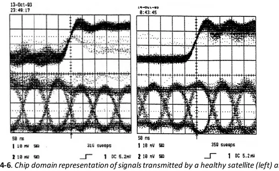
- [Pagot et al., 2015] presented at ION ITM 2015 conference shows nominal distortions that affect GPS L1 C/A signals on the chip domain and the correlation function domain from high-gain dish antennas data collections.

- [Pagot et al., 2016a] presented at Navitec 2016 conference also focuses SQM design for Galileo E1C and Galileo E5a signals.

- [Pagot et al., 2016b] presented at ION ITM 2016 conference exposes a strategy to design TM and this strategy is used to define TM on Galileo E5a and Galileo E1C signals.

- [Pagot et al., 2016c] presented at ION GNSS+ 2016 conference deals with the SQM design for Galileo E1C and Galileo E5a signals.

- [Thevenon et al., 2014] presented at Navitec 2014 conference gives details on the chip domain observable and on its capacity to visualize non-nominal distortions.

- [Julien et al., 2017] accepted to be presented at ION ITM 2017 conference presents an extended TM definition and its associated SQM.

1.4 Thesis Outline

31

1.4 Thesis Outline

The dissertation is structured as follows:

Chapter 2 introduces the background which permits to understand the GNSS signal distortions problematic. A general overview of GNSS is given before exposing the civil aviation context which is focused in this Ph.D.. More precisely ICAO requirements definitions are presented and concepts of augmentation systems, crucial to meet these stringent requirements, are described. Finally the SBAS is presented as it is the original augmentation system targeted in this study.

Chapter 3 is a more technical chapter which synthetizes the GNSS receiver processing. This chapter is important because it gives the background necessary to understand how a GNSS signal is processed and explains the impact of a signal distortion on the final pseudorange measurement. The analog and the digital sections of the receiver are presented separately. In addition, GNSS signals of interest are presented: GPS L1 C/A, Galileo E1C, Galileo E5a pilot component and GPS L5 pilot component. Mathematical time-domain expression, power spectral density and correlation function of the different signals are provided.

Chapter 4 is the first chapter dedicated to signal distortions. First of all, nominal and non -nominal distortions are described based on the state-of-the-art. This description includes a speculation about the origin of these distortions on GPS L1 C/A signal. Secondly, different impacts of signals distortions on the receiver processing are listed. Then, the issue related to non-nominal distortions in a civil aviation context is detailed. It is seen that it is necessary to model and detect non-nominal distortions that could affect a GNSS signal. Finally, this chapter describes in details two strategies to observe signal distortions: look at distortions in the chip domain and look at distortions on the correlation function. Chapter 5 synthetizes results on nominal distortions obtained by the observation of real data collections from high-gain dish and from omnidirectional antennas. After a brief introduction to the different setups that were used to collect the different GNSS signals, the effects of nominal distortions at different levels of the receiver processing are observed. From data collected with high-gain dish antennas on GPS L1 C/A and Galileo E1C signals, three observables are used to quantify the impact of signal distortions on users: the chip domain, the correlation function and the S-curve zero-crossing. From high-gain dish antenna measurements, it appears that a wrong or an absence of antenna calibration induces an additional distortion on the measurement which cannot be separated from the nominal distortion generated by the payload. This is the reason why the S -curve zero-crossing observable is also provided based on measurements collected on GPS L1 C/A signal with an omnidirectional antenna. This kind of antenna does not need any calibration because a normalization can be achieved using all visible signals collected at a given time. Finally, inter-PRN tracking biases are estimated from the omnidirectional antenna data collection and appear consistent with results provided in the state-of-the-art.

Chapter 6 deals with the proposition of new TMs for Galileo E5a, Galileo E1C and GPS L5. After a detailed description of the current GPS L1 C/A TM adopted by ICAO, it is proposed to assume that same parameters are relevant to characterize threatening distortions on new modulations. Based on two criteria (the impact of a distortion on a reference station and the impact of a distortion on differential users) the parameters range is limited. Finally TMs similar to the ICAO GPS L1 C/A A, B and TM-C are proposed for each signal of interest.

32

Chapter 7 is a thorough study of SQM on new modulations regarding TMs proposed in the previous chapter. Firstly, definitions provided by ICAO on SQM are presented. Secondly an innovative method is exposed that is able to test and compare theoretically the SQMs performance whatever the received signal 𝐶 𝑁⁄ 0 is. Then, based on this representation and on TMs proposed in chapter 6, performances

of reference SQMs are assessed for the different signals. Finally, a method to optimize the SQM is described. The aim is to reduce the number of SQM metrics still reaching targeted performances. Chapter 8 draws conclusions from main results of this Ph.D. and makes recommendations for works that could be addressed in the future.