an author's https://oatao.univ-toulouse.fr/22873
Beauregard, Laurent and Blazquez, Emmanuel and Lizy-Destrez, Stéphanie Optimized transfers between Earth-Moon invariant manifolds. (2019) In: 27th International Symposium on Space Flight Dynamics (ISSFD), 24 February 2019 - 27 February 2019 (Melbourne, Australia).
18th Australian Aerospace Congress, 24-28 February 2018, Melbourne
18th Australian International Aerospace Congress
Optimized transfers between Earth-Moon invariant
manifolds
Laurent Beauregard 1, Emmanuel Blazquez 1, Stéphanie Lizy-Destrez 1
1 Institut Supérieur d’Aéronautique et de l’Espace (ISAE-SUPAERO), 10 Avenue Edouard Belin, 31400 Toulouse
Abstract
Launching its first module in 2022, the upcoming Lunar Orbital Platform-Gateway (LOP-G) or simply the Gateway will be a space station assembled in cis-lunar space, most likely on a Near Rectilinear Halo Orbit (NRHO). The best transfer strategy to the LOP-G remains an open question, one candidate involves going to an intermediate Halo as a parking orbit. The focus of this work is on the transfer methodology between Halo orbits. Two burns direct transfers can provide simple transfer trajectories, however when longer transfer time is permitted, structures of the natural dynamics of the Earth-Moon system, such as manifolds, can be exploited for transfers with lower cost in velocity increment . In this work, low thrust trajectories, Lambert arcs and new manifold intersection methods will be compared for the lowest cost .
Keywords: Earth-Moon system, Manifolds, Transfer, NRHO, Optimization
1. Introduction
The International Space Exploration Coordination Group (ISEGC), composed of most of the international space agencies, has agreed on deploying a space station in cis-lunar space, called the Lunar Orbital Platform-Gateway (LOP-G), as a gateway to enable deep space exploration [1]. The most likely position of the LOP-G will be a L2 southern Near Rectilinear Halo Orbit
(NRHO) of apoapsis 1500 km above the surface of the Moon. The NRHO is a particular case of the family of Halo orbits which exist in the Circular restricted three body problem (CR3BP). One of the common metric when analysing orbital transfers is the of the maneuver, the change in velocity necessary to perform the transfer. Although some work has been done for the best transfers in the dynamics of cis-lunar space [2] there still is an open question as to the optimal transfer strategy. One method to reach the orbit of the LOP-G is to go unto an intermediate Halo orbit, acting as a parking orbit. In this article, three transfer methods will be compared for the best to travel across Halo orbits. The first method will consider a long series of maneuvers of low to “jump” along the Halo family. The second method will be a classic case of optimized Lambert arcs. The last method will consider invariant structures of the Halo orbits, called unstable and stable manifolds and their intersections. While such structures have been used before [3], this article will present a new methodology to obtain a one-dimensional subset of intersections.
2. Circular Restricted Three Body Problem
The only gravitational bodies considered in this article are the Earth and the Moon; furthermore, the Moon is approximated to move in a circular orbit around the Earth-Moon barycenter. Spacecrafts or stations moving in this environment are considered massless. This framework is called the CR3PB for the Earth Moon system and has been extensively studied. The data for this system can be found in table 1.
Table 1. Data
Symbol Value Units
Earth’s gravitational parameter 398600.4415 Moon’s gravitational parameter 4902.8005821478
The frame chosen has the following properties
The Earth-Moon barycenter is located at the origin.
The frame rotates in such a way that the Earth’s and Moon’s position are stationary
The Moon is located on the +x axis (x > 0, y = 0, z = 0)
The Earth is located on the –x axis (x < 0, y = 0, z = 0)
The direction of rotation of the Moon is counterclockwise as seen from above (z-axis)
The y direction is chosen to create a right handed coordinated system
The unit vectors ̂ ̂ ̂ correspond to the +x, +y and +z direction respectively. In this framework the angular rotation of the Moon is
⃗⃗ √
̂
(1)Due to simple kinematics, the location of the of the Earth and Moon can be shown to be
̂
̂
(2)The equations of motion of a third massless body, whose position and velocity are respectively, are given by
(3)
| |
| |
⃗⃗
⃗⃗
⃗⃗
(4)3. Theory of Halo orbit
Several types of closed orbit of the CR3PB exists [4]. The ones that are of interest in this study are called Halo orbits, they exists as bifurcations of the planar Lyapunov orbit associated with the Lagrangian points L1, L2 or L3. Different parameterization of these orbits
are possible, the most common parameterization comes from applying the Poincaré-Lindstedt method to the linearized equation of motion and by varying the amplitude of the out-plane motion until the in plane and out of plane frequency of the motion are equal [4]. While this method is perfectly valid, it suffers from the drawback of being a one way function from to the orbital states ( ). In other words, given the orbital states of the Halo orbit ( ), it is very difficult to obtain the which produced this orbit. In this article the parameterization used is the out of plane component of the velocity at the x-y plane ( crossing. Every Halo orbit is uniquely characterized by this variable. This has the advantage of being obtainable from the state variables ( ) alone in a straightforward way. Another common parameterization is the smallest distance from the orbit to the Moon’s surface, called the periapsis . For reference, figure 1 shows the relation between and . Figure 2 shows the relationship between and .
Figure 1. Relation between the Figure 2. Relation between the
18th Australian Aerospace Congress, 24-28 February 2018, Melbourne
It was found that up to an of roughly 60,000 km, an approximately linear relation is satisfied given by equation 4.
(4)
An approximate relationship between and was found to given by equation 5.
√ (5)
Where is in units of 1000 km and is in m/s.
4. Energy of orbits
A well-known constant of motion for the CR3PB is the energy (a.k.a Jacobi constant). Its expression is given by| | | |
⃗⃗
(6) For the L2 family, the energy increases from a minimum near
their bifurcation with the planar Lyapunov orbit and reaches a maximum around , it then falls back down. This behavior is shown in figure 3.
This property of several orbits having the same energy will be exploited later when considering transfers from different Halos.
5. Low thrust approach
Concerning orbital transfers between orbits, two limiting cases are often considered, the case of infinite thrust with instantaneous maneuvers or the case of infinitesimal thrust with infinitely long maneuvers. Each limiting case has an associated to it. For the case of two body orbital dynamics with central body gravitational parameter , the optimal transfer between two circular co-planar orbit of radius and is given by the Hohmann transfer. The cost of the Hohmann transfer is denoted by whereas the low thrust trajectory has cost denoted .
Their difference can expanded to the lowest nonzero order in and can be shown to be
√
(7)The conclusion is that, in terms of , a low thrust transfer can be well approximated by a Hohmann transfer, and vice versa, for orbits that are close. One can therefore approximate the cost of a low thrust trajectory by a series of impulsive transfers going along a continuous family of closed trajectory from the initial orbit to the final orbit. This is precisely the methodology used in the article to estimate the low thrust .
Given a sampling of the L2 Halo family, which is finely spaced enough to approximate low
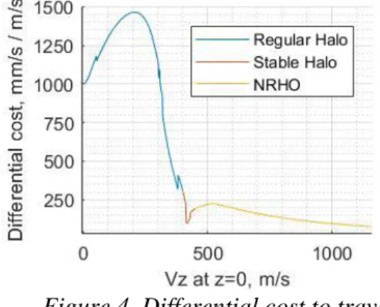
thrust cost, the algorithm described above can used to establish a baseline for the between any two Halo orbits. It does so by “jumping” in between every Halo orbits of the family connecting the starting and end orbit. The results obtained for this procedure are summarized in figure 4 and 5.
Figure 3. Jacobi constants for the L2 Southern Halo orbit
Figure 4. Differential cost to travel Figure 5. Cumulative cost to
between neighboring orbit travel from to any
Figure 4 shows the differential cost
of traveling between two close orbits. Figure 5 shows the cumulative cost to travel between orbits with to . The whole Halo family can be covered with roughly 560 m/s. In particular, the NRHO family only requires at most 100 m/s to cover.
6. Lambert arcs
Given a dynamical system, such as the CR3PB, two points in space, & , and two times, & , the Lambert problem consists in finding a curve that satisfies the dynamics of the system, such that & , this is also equivalent to finding the velocity
̇ that produces the trajectory above. In the case of two body orbital mechanics this problem has been fully solved. For the CR3PB, there is no known analytical solution, and one must resort to a numerical approach. One method is based on the fact that considering small enough Time Of Flight ( ), one possible trajectory can be approximated by a line connecting the initial point and final point , with initial velocity approximated by
.
A Newton’s method can then be used to correct until is obtained. Thenext step involves incrementally increasing the , using the previous as a guess and correcting the trajectory at each step, until the desired is obtained (or one with least is obtained).
7. Manifold method
7.1 Manifold generation
The stability of a given Halo orbit can be analyzed by the eigenvalues of the differential of the Poincaré map [5]. The magnitude and phase of these eigenvalues for the L2 family are shown
in figure 6.
18th Australian Aerospace Congress, 24-28 February 2018, Melbourne
Three different regions of stability are observed, regular Halos from are unstable, neutral Halos from are stable, and lastly, NRHOs from are again unstable.
Given an unstable direction with eigenvalue | | , perturbations along this direction grow exponentially with each period, with the initial perturbation. After revolutions
(8)
The set of trajectories generated by all unstable directions is called the unstable manifold of the orbit. Being unstable, these trajectories can be achieved with a small . Analogously, the stable manifold can be generated with all stable directions | | , these converge to the Halo orbit with each revolution. When time is propagated backward, the unstable and stable trajectories invert behavior and the trajectories on the unstable manifold converge to the Halo and the stable manifold diverges from the Halo. Points on these manifolds can be described by two parameters , a perturbation size and a time of flight .
7.2 Manifold Intersection
One method for a spacecraft to travel from Halo A to Halo B using their manifolds is to insert into the unstable manifold of A, wait for some (to be solved for) amount of time, then perform a maneuver to insert into the stable manifold of B and thus converging to the final orbit. The main challenge of this method is the determination of the intersection point between the two manifolds; this problem is equivalent to solving for the combination and which has the same positions.
(9)
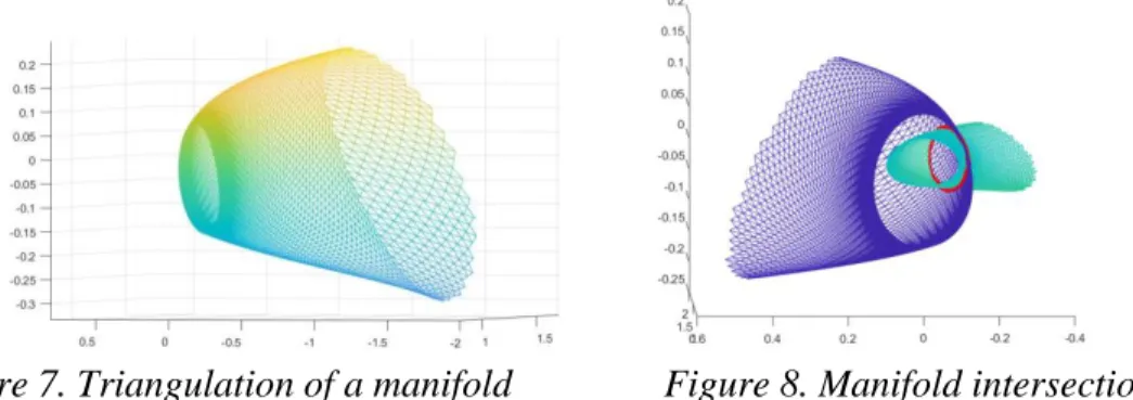
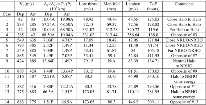
Because one is searching the intersection of two surfaces in space, it is expected that the intersection is generally a one dimensional object. The method employed in this article involves computing several arcs of the manifolds, typically on the order of 100, at regularly spaced intervals in time. From this grid in , a triangulation is performed as shown in figure 7.
Figure 7. Triangulation of a manifold Figure 8. Manifold intersection
Intersections between two triangulated surfaces can be computed efficiently with a Möller triangle-triangle intersection algorithm [6]. Such intersections are shown in figure 8. From these intersections, the velocities can be obtained by a linear regression applied on the intersecting triangles followed by a differential correction to obtain more accurate intersections. From this set of intersections, the one with least is chosen.
8. Results
Fourteen different cases were considered in this article, covering a wide range of qualitatively different scenarios, the three transfer methods were applied. The applies to the Lambert transfer.
Table 2. Comparison of the three transfer methods
Vz (m/s) Az (A) or Pe (P) (103 km) Low thrust (m/s) Manifold (m/s) Lambert (m/s) ToF (hours) Comments Case Dep Arr Dep Arr
1 42 83 10.04A 19.98A 48.92 49.76 48.55 125.03 Close Halo to Halo 2 233 285 57.24A 68.50A 72.13 69.32 72.56 128.82 Close Halo to Halo 3 42 285 10.04A 68.50A 331.02 312.28 340.72 119.6 Far Halo to Halo 4 285 42 68.50A 10.04A 331.02 312.44 356.64 138.8 Opposite of #3 5 549 635 7.03P 4.71P 17.09 18.42 17.05 121.84 Close NRHO-NRHO 6 793 885 2.32P 1.49P 11.44 12.33 11.48 91.74 Close NRHO-NRHO 7 549 885 7.03P 1.49P 53.41 61.87 54 105.18 Far NRHO-NRHO 8 885 549 1.49P 7.03P 53.41 59.1 52.84 111.55 Opposite of #7 9 424 885 13.64P 1.49P 79.15 N/A 83.39 134.71 Neutral Halo
to NRHO 10 885 424 1.49P 13.64P 79.15 N/A 81.51 130.63 Opposite of #9 11 316 587 72.21A 5.88P 80.3 33.75 44.98 340.16 Halo to NRHO same energy 12 587 316 5.88P 72.21A 80.3 33.78 54.89 293.56 Opposite of #11 13 275 883 66.5A 1.51P 173.05 81.71 110.11 281.95 Halo to NRHO same energy 14 883 275 1.51P 66.5A 173.05 80.3 146.2 209.11 Opposite of #13 It is clear that when the departing and arriving orbits are close in space, the three methods give essentially the same , differing by less than 10%. However for orbits that differ significantly, the manifold method can provide improvement over Lambert arcs. The instances where the manifold method dominates are for transfers between orbits with the same energy #11-12-13-14, reducing the cost between 25% and 45% as compared to Lambert arcs.
9. Conclusion
In this article, three methods of transfer between L2 Halo orbits have been considered; a low
thrust approximation, a two burn optimized Lambert arc and a manifold intersection method. The low thrust approximation provides a benchmark of the required to compare other methods. For orbits that are close, there is little difference in the outcome of the three methods. However, it has been shown that for far orbits, the manifold method can reduce significantly the cost , by up to 45%. Further studies should increase the degree of freedoms available to the algorithm by also considering the central Eigenspace.
References
1. P. Guardabasso et al, “Lunar outpost sustaining human space exploration by utilizing in-situ resources with a focus on propellant production,” International Astronautical Congress 2018, IAC-18,A5,1,5,x46282.
2. S. Lizy-Destrez, “Rendezvous optimization with an inhabited space station at EML2,” 25th International Symposium on Space Flight Dynamics, ISSFD, 2015.
3. G. Gomez et al, “Connecting orbits and invariant manifolds in the spatial restricted three-body problem,” Caltech, 2004.
4. S. K. Wang et al., “Dynamical systems, the three-body problem and space mission design,” Caltech, 2000.
5. Norman R. Lebovitz, “Ordinary differential equations, chapter 9 stability ii:maps and periodic orbits,” http://people.cs.uchicago.edu/ lebovitz/odes.html.