Model selection for degradation modeling and prognosis with health monitoring data

OATAO is an open access repository that collects the work of Toulouse

researchers and makes it freely available over the web where possible

Any correspondence concerning this service should be sent

to the repository administrator:

tech-oatao@listes-diff.inp-toulouse.fr

This is an author’s version published in: http://oatao.univ-toulouse.fr/19980

To cite this version:

Nguyen, Thi Phuong Khanh

and Fouladirad, Mitra and Grall,

Antoine Model selection for degradation modeling and prognosis

with health monitoring data. (2017) Reliability Engineering and

System Safety, 169. 105-116. ISSN 0951-8320

Official URL:

http://dx.doi.org/10.1016/j.ress.2017.08.004

Open Archive Toulouse Archive Ouverte

Model

selection

for

degradation

modeling

and

prognosis

with

health

monitoring

data

Khanh

T.P.

Nguyen

_,

_Mitra

_Fouladirad

_,

_Antoine

_Grall

Keywords:

Model selection Prognostic prediction Residual life prediction Degradation process Lévy process

a b s t r a c t

Healthmonitoringdataareincreasinglycollectedandwidelyusedforreliabilityassessmentandlifetime pre-diction.Theynotonlyprovideinformationaboutdegradationstatebutalsocouldtracefailuremechanismsof assets.Theselectionofadeteriorationmodelthatoptimallyfitsinwithhealthmonitoringdataisanimportant issue.Itcanenableamorepreciseassethealthprognosticandhelpreducingoperationandmaintenancecosts. Therefore,thispaperaimstoaddresstheproblemofdegradationmodelselectionincludinggoals,procedureand evaluationcriteria.FocusingoncontinuousdegradationmodelingincludingsomecurrentlyusedLévyprocesses, theperformanceofclassicalandprognosticcriteriaarediscussedthroughnumerousnumericalexamples.We alsoinvestigateinwhatcircumstanceswhichmethodsperformbetterthanothers.Theefficiencyofanewhybrid criterionishighlightedthatallowstotakeintoaccounttheinformationofgoodness-of-fitofobservationdata whenevaluatingprognosticmeasure.

1. Introduction

Degradationmodelinginthepresenceofhealthmonitoringdatais extremelyimportantforlifetimeprognosisandmaintenanceplanning. Complexmodelspermittotakeadvantageofallavailableinformation anddescribeprecisely thedynamics of degradation.However,these modelsarenoteasily tractable,andtheircalibrationin thepresence ofdataisaburdensometask.Ontheotherhand,averysimplemodel whichcanbeeasilyfittedtodatabutcanunderestimateoroverstate theuncertaintyaroundthelifetimeprediction.Thislattercaninduce risks and additional costs in prognosis based decision making and maintenance. A useful and suitable degradation model leads to a balancebetweenaccuracyandtractability,[1,2].

Thedegradation considered asa random phenomenon often has a gradual time-continuous trajectory. Regarding the system under consideration,thedegradation cantake values in discreteor contin-uousspace. Forinstance, in acrack growthphenomenon, thecrack lengthcan takeinfinitepossible valuesassoonasitbeginstogrow. Similarly,adeterioratingproductionprocesscanhaveseveralquality stateswhichwillimpacttheproductionandresultofgainorlosses.In thesetwocases,themodelingprocedureshouldtakeintoaccountthe phenomenonunderconsideration,seeforinstance[3–5].

Thispaperfocusesonthegradualdegradationmodelingand progno-siswithhealthmonitoringdata.Whendataisavailable,theimportant issueistoselectthemodelwhichdescribestheunderlyingdegradation

∗ Corresponding author.

E-mail addresses: thi_phuong_khanh.nguyen@utt.fr , nguyenthipk85@gmail.com (K.T.P. Nguyen), mitra.fouladirad@utt.fr (M. Fouladirad), antoine.grall@utt.fr (A. Grall). phenomenonin thebest possible way. Thedataarecollected under given environmental conditions and may not represent the average behavior of the deteriorating system. A suitable model is one who cantakeintoaccountthepossibilityofextremebehaviorsduringdata collectionwithoutlosing inperspectivetherealaveragedegradation behavior.Thefinaluseofthedegradationmodelcanlargelyimpactthe waydataishandled,andamodelisfavored.Iftheresultofmodeling hasalargeimpactonsafetyissues,thechoiceandtheprocedureare notcarriedoutinthesamewayasifonlyeconomicprofitsorlosses aretakenintoaccount.Similarly,thecostinducedbydecisionpolicies basedondifferentmodelsmayinfluencethemodelselection.Regarding statisticalproperties,thebestcandidateiswellcharacterizedfromdata trajectories.Itcanpermitfastcalibrationandstraightforwardlifetime estimation.Formoredetailsandexamples,referto[6,7].

Tobeabletodiscardirrelevantmodelsitisnecessarytohavesome priorknowledgeaboutthedegradationphenomenonunder considera-tion.Inthepresenceofsuchinformationanddegradationdata,thegoal ofdegradationmodelingistoselectonemodelfromasetofcompeting modelsthatbestcapturestheunderlyingdegradationprocess.Asitis mentionedbeforetheselectioncriteriadependmainlyonthespecific purposeforwhichthemodelcanbeused,seeforinstance[5,8].

ThispaperdealspartlywithLévyprocesses[9]andfocusesonthe mostcommonlyusedwhichareWienerandGammaprocesses.Model calibrationanddatafittingofthesemodelshavebeenwidelyaddressed

in the fields of finance, biology andengineering [10,11]. However, themodelselectioncriteriainthefinanceandbiologyfieldhavesome differences with engineering domain wheremaintenance and safety constraintsaresignificantconcerns[5,12,13].Themodelselectionfor engineeringpredictionproblemsisanimportantissuebuthasnotbeen generalizedandextensivelyaddressed,[14].

Thispaperproposesdifferentcriteriaformodelselection,toavoid system failure andwith themost reasonablecalculation time. First, anoverviewoftheconsideredstochasticprocessesisgiven,andtheir use indegradation modeling is underlined.Afterwards, toprovide a first selectioncriterion and tocontinue tooutline a methodological guide,somewidely addressedandwellknownstatisticaldatafitting criteriaarepointedout.Theirlimitsandperformancesarehighlighted, and new prognostic basis criteria are introduced. To complete the methodological task,the proposed procedure is applied todifferent simulateddatasets.Thebehavior,weakness,andperformancesofthe modelselectionareanalyzedanddiscussed.

Theremainder of thepaperis asfollows. Section2describes the set of models underconsideration. In Section3, the criteria for the data-basedmodelselectionareexposed.Section4givessomeprognosis criteria.Eventually,inSection5theproposedmodelsandcriteriaare testedonsimulateddata.

2. Stochastic degradation modeling and parameter estimation This section focuses on the considered Levy processes in the framework of degradation modeling, [12,15,16]. A Lévy process is a stochastically continuous processwith stationary andindependent increments.ItcanbedecomposedintothesumofadriftedBrownian motionandajumpprocesssuchasGammaorPoissonprocess.These propertiesmakethisclassofprocessesagoodcandidatefordegradation modeling.Inthis paper,thewidelyusedLevyprocesses,particularly BrownianandGammafamily,arethemodelsunderconsiderationto describethedegradationbehavior.Theyarepresentedinthefollowing. Letusintroducesomenotations.LetX_tbethedegradationlevelofthe systemattimet.LetLbethefailurethresholdinthesensethatthe sys-temissupposedtobefailedifthedegradationlevelexceedsthelevelL. Lettps(L)bethefirstpassagetimeofthedegradationprocesstolevelL:

𝑡_𝑝𝑠(𝐿)=inf{𝑡∈ ℝ+ ,𝑋_𝑡≥𝐿}. (1)

Theresidualusefullifetime(RUL)attimetgiven𝑋_𝑡=𝑥denotedby RUL₍ x,t) isthetimedurationbeforethefirstpassagetimetps(L)starting fromthedegradationlevelxatt.Inthefollowingt_ps(L)willbedenoted

t_psexceptincaseofambiguity.

2.1. Lévytypediffusionprocess

Toconsider ageneral degradationmodeling frameworkandtake into account the possible existing physical models, it is natural to introducestochasticdifferentialequations(SDE) basedonastandard BrownianmotionsB_t:

𝑑𝑋_𝑡=𝑚(𝑋_𝑡,𝑡)𝑑𝑡+𝜎(𝑋_𝑡,𝑡)𝑑𝐵_𝑡,

(𝑚,𝜎)∶ℝ× ℝ+ ↦ ℝ are respectively the drift and the diffusion co-efficient. These equations appear at the beginning of 20th century in statisticalmechanicsandhave beenthoroughlyformulated byItô

[17,18].Suchequationscanbederiveddirectlyfromexistingphysical models by adding Gaussian “white noises” on measurements. They permitawiderangeofdegradationmodelingduetotheflexibilityof thestructureandfunctionalparameters.

Inthissection,somespecificLevydiffusionsprocessesarepresented, andtheirinterestindegradationmodelingisunderlined.Foreachcase, thedifferentialequation,therelateddistributionfunctions,andsome statisticalpropertiesareexposed.

2.1.1. Wienerprocess

TheWienerprocess isvery populardeteriorationmodeling when observationsincrementsvarynon-monotonically.Thestatistical prop-ertiesofthefailure timein thecaseofaWienerprocessarestudied in [19,20].It hasbeenconsidered inreliabilityandlifetimeanalysis widelysincethe1970s.Authorsin[21]usedtheWienerprocesswith drifttomodelacceleratedlifetesting data. In[22,23]theimpact of measurementerrorsontheWienerdegradationmodelofself-regulating heating cables is analyzed. Authors in [24–26] also focused on the stopping time(failure time) of Wienerdeterioration modelsand ex-pandedtheexistingtheoreticalresultsinthis domain.TheBrownian motionwithnon-lineardrifthasattractedmoreattentioninengineering problemsandresiduallifetimeestimation,seeforexample[27–29].

Moreprecisely,adiffusionprocessinBrownianmotionfamilyhas thefollowingproperties.Theincrementsareindependent,X_tissolution of theSDE𝑑𝑋_𝑡=𝜇(𝑡)𝑑𝑡+𝜎𝑑𝐵_𝑡,where𝜇(t) is afunction of tandBt is a standardBrownian motion.The transitionprobability to 𝑋_𝑡=𝑥

knowingthat𝑋_𝑠=𝑦isgivenby:

𝑝(𝑥,𝑡|𝑦,𝑠)=√ 1 4𝜋𝜎(𝑡−𝑠) 𝑒𝑥𝑝 ( −(𝑥+𝑀(𝑡,𝑠)−𝑦) 2 4𝜎2 (𝑡−𝑠) ) , (2)

whereM(t,s),𝛾(t,s)aregivenby:

𝑀(𝑡,𝑠)=−_∫ 𝑡

𝑠

𝜇(𝑢)𝑑𝑢, (3)

ThemeanandvariancevaluesofX_taregivenby:

𝔼[𝑋_𝑡]=−𝑀(𝑡,0),Var[𝑋_𝑡]=𝜎2 𝑡 (4)

M1:Wienerprocesswithlineardrift. Thisprocessisthespecialcaseofa

Wienerprocesswhenthedriftandthevariancearenottimedependent (𝜇(𝑡)=𝜇isconstant).ThisdiffusionprocesswhichisalsoaLévyprocess

is suitable for fluctuating degradation recordslinearly increasing in time.ItwillbereferredasM₁ inSection5.

TheRULcumulativedistributionfunction(cdf)foradrifted Brown-ianmotiongiventheobservationvalue𝑋_𝑡=𝑥attheobservationtime taregivenasfollows[30]:

𝐹_{𝑅𝑈 𝐿(} 𝑥,𝑡) (𝑢)=Φ ( −𝐿+𝜇𝑢+𝑥 𝜎√𝑢 ) +𝑒2 𝜇 𝜎2(𝐿−𝑥)Φ ( −𝐿−𝜇𝑢+𝑥 𝜎√𝑢 ) (5)

whereΦ(· )isthestandardnormalcumulativedistributionfunction.

M2: Wiener processwith time-dependentdrift. This processis the

par-ticular case of a diffusion process when the degradation process is exponentiallyincreasingintime(𝜇(𝑡)=𝑎𝑡𝑏_{).ItwillbereferredasM}

2 in Section5. Inthis case,theratiobetween its driftanddiffusionis notaconstantandalsodependsonthetime.Therefore,itisdifficult toderivetheexplicitexpressionoftheRULdistribution.Itsevaluation requiressolving anon-singular Volterra Integral Equation.It canbe donenumerically,seee.g.[31].

2.1.2. M3:diffusionprocesswithpurelytime-dependentdriftanddiffusion

Thisprocessistheparticularcaseofadiffusionprocesswhen𝜇(t)

and𝜎(t)aretimedependentfunctionsindependentofX_t).Thisissuitable foradegradationprocessincludingrandomwalkswithtime-dependent driftanddiffusionterms.Inthispaper,weconsideraspecialcaseofthe purelytimedependentdriftanddiffusionBrownianmotion:𝜇(𝑡)=𝑐𝑎𝑡𝑏 and𝜎(𝑡)=√2𝑎𝑡𝑏_{.ItwillbedenotedasM}

3 inSection5.Asthepower-law driftisproportionalwithdrift,accordingto[32],theRULCDFofthe processattimetgivenadegradationlevelattimet,𝑋_𝑡=𝑥,isderived: 𝐹𝑅𝑈 𝐿(𝑥,𝑡)(𝑢)=Φ ( −𝐿−𝑐𝛾(𝑡𝑝𝑠,𝑡)+𝑥 √ 2𝛾(𝑡𝑝𝑠,𝑡) ) +𝑒𝑐( 𝐿− 𝑥) _Φ ( −𝐿−𝑐𝛾(𝑡𝑝𝑠,𝑡)+𝑥 √ 2𝛾(𝑡𝑝𝑠,𝑡) ) (6)

2.1.3. M₄ :Ornstein–Uhlenbeckprocess

A time-dependent Ornstein–Uhlenbeck (OU) Process is widely usedto describephysical dynamicsof systemswhich stabilize atits equilibriumpoint.Inthefieldofreliabilitymodeling,OUprocesscould bea goodcandidateformodelingthedegradation processwhenthe drift is time-dependent and also depends on the degradation state

[31,33].IndeedforcommonlyusedprocessessuchasdriftedBrownian motion[30],themeanorthedrifttrendcan bechosenquitefreely, butthevariancestronglydependsonthestochasticprocessproperties. Tocontrolthevariancefunctionindependentlyofthemeantendency, atime-dependentOUprocessisagoodcandidate.Theincrementsof Ornstein–Uhlenbeckprocessareindependent,X_tissolutionoftheSDE:

𝑑𝑋_𝑡=(𝜆(𝑡)𝑋_𝑡+𝜇(𝑡))𝑑𝑡+𝜎(𝑡)𝑑𝐵_𝑡,where𝜆(t),𝜇(t)and𝜎(t)arefunctions int.Thetransitionprobabilitydensityfunctionfrom𝑋_𝑠=𝑦to𝑋_𝑡=𝑥

isgivenby: 𝑝(𝑥,𝑡|𝑦,𝑠)= 𝑒𝛼 (𝑡,𝑠) √ 4𝜋𝛾(𝑡,𝑠) 𝑒𝑥𝑝 ( −(𝑥𝑒 𝛼(𝑡,𝑠)_{+𝑀(𝑡,𝑠)−𝑦)}2 4𝛾(𝑡,𝑠) ) (7)

where𝛼(t,s),M(t,s),𝛾(t,s)aregivenby:

𝛼(𝑡,𝑠)=−_∫ 𝑡 𝑠 𝜆(𝑢)𝑑𝑢,𝑀(𝑡,𝑠)=−_∫ 𝑡 𝑠 𝜇(𝑢)𝑒𝛼(𝑢,𝑠)_{𝑑𝑢,𝛾(𝑡,𝑠)=} ∫ 𝑡 𝑠 𝜎2 (𝑢)𝑒2 𝛼( 𝑢,𝑠) 2 𝑑𝑢 Inthispaper,weconsideraspecialcaseofOUprocess,denotedas

M₄ anddefinedby:

𝜆(𝑡)=𝑎,𝜇(𝑡)=𝑚′(𝑡)−𝑎_{⋅ 𝑚}(𝑡),𝑚(𝑡)=𝑏𝑡𝑐_{, 𝑐≥1,𝜎(𝑡)=𝑑 (8)}

Theremaining usefullifetimepdf of this OU processcan be nu-mericallyevaluatedasthesolutionofanon-singularVolterraintegral equation,see[33].

2.2. Gammaprocess

Thegammaprocessisapositivestochasticprocesswithindependent increments.Henceitisusefultodescribethedeteriorationcausedby theaccumulationof wear[34].Thisprocessisajumpprocesswhich can beroughly consideredasa successionof thefrequent arrivalof tiny increments. This rough description makes it relevant to model gradual deterioration such as corrosion, erosion, wear of structural components,concretecreep,crackgrowth[35].Moreover,thegamma processhasanexact probabilitydistribution functionwhich permits feasiblemathematicaldevelopments.Thisprocesshasbeenwidelyused indeteriorationmodelingforcondition-basedmaintenance(see[12]).

Theincrementsofagammaprocess(X_t),𝑋_𝑡−𝑋_𝑠,areindependent, 𝑋_𝑡−𝑋_𝑠∼ 𝐺𝑎(𝛼(𝑡)−𝛼(𝑠),𝛽) with the transition probability density functionfrom𝑋_𝑠=𝑦to𝑋_𝑡=𝑥asfollows:

𝑝(𝑥,𝑡|𝑦,𝑠)= 𝛽 𝛼( 𝑡)− 𝛼( 𝑠) Γ(𝛼(𝑡)−𝛼(𝑠))(𝑥−𝑦)

𝛼( 𝑡)− 𝛼( 𝑠)−1 _𝑒−( 𝑥− 𝑦) 𝛽 ₍₉₎ wheretheshapefunction𝛼(t)isanincreasingfunctiondefinedonℝ+ . ΓistheEuler’sGammafunction.and𝛽thescaleparameter.Themean

andvariancevaluesofX_taregivenby: 𝔼[𝑋_𝑡]=𝛼(𝑡)

𝛽 , Var[𝑋𝑡]=

𝛼(𝑡)

𝛽2 (10)

The choice of 𝛼(.) and 𝛽 allows to model various deterioration

behaviorsfromalmostdeterministictoverychaotic.Notethat,based ontheformof𝛼(t),theGammaprocesscanbe:

• Homogeneous Gamma Process if 𝛼(t) is a linear function in t: 𝛼(𝑡)=𝑎𝑡.ThisprocessisdenotedM₅ .

• Non-homogeneousGammaProcessif𝛼(t)isanon-linearfunction: forinstance𝛼(𝑡)=𝑎𝑡𝑏,a>0,b>1fortheprocessreferredasM₆ in

thefollowing.

Givenadegradationlevel𝑋_𝑡=𝑦attimet,thecumulative distribu-tionoftheremainingusefullifeofagammaprocessisgivenby[36]:

𝐹_{𝑅𝑈 𝐿(} 𝑦,𝑡) (𝑢)=

Γ(𝛼(𝑢+𝑡)−𝛼(𝑡),(𝐿−𝑦_𝑡)∕𝛽) Γ(𝛼(𝑢+𝑡)−𝛼(𝑡)) ;

Γ(⋅,⋅) istheupperincompleteGammafunction. (11)

2.3. Parameterestimation

Parameter estimation refers tothe process of using sample data (degradationrecordsatobservationtimes)todeterminethevaluesof themodelparametersthatbestfitsthedata.Theparameterestimation of Lévy processes is discussedin [37]. Among numerous parameter estimationmethods,theMaximumLikelihoodEstimation(MLE)isone ofthemostwidelyused[38].Itproposesaunifiedapproachtoselect thesetofvalues of themodelparametersthrough themaximization of the likelihood function. Intuitively, this maximizes the matching betweenthechosenmodelandtheobserveddata.

Suppose thatthedegradation recordshavebeen obtainedfrom n

identical independentcomponents.Let ml be the numberof records collectedonthelthcomponent(1≤l≤n)andassumem_l≥2.Then,x_lj

isthedegradationrecordsofthelthcomponentatthejthobservation time (1≤j≤ml). Recall that 𝑝𝜃(𝑥𝑙𝑗,𝑡𝑙,𝑗|𝑥𝑙𝑗−1 ,𝑡𝑙𝑗−1 ;𝜃) is the transition probabilitydensityfunctionofthedegradationprocessknowingthat𝜃

isthevectorofmodelparameters.Thelog-likelihoodfunctionforthe wholeuncensoredsampledatasetisgivenby:

𝐿(𝜃)= 𝑛 ∑ 𝑙=1 log(𝑝_𝜃(𝑥_𝑙1 ,𝑡_𝑙1 |𝑋0 ,0);𝜃))+ 𝑛 ∑ 𝑙=1 𝑚𝑙 ∑ 𝑗=2 log(𝑝_𝜃(𝑥_𝑙𝑗,𝑡_𝑙𝑗|𝑥𝑙( 𝑗−1) ,𝑡𝑙( 𝑗−1) ;𝜃)) TheobjectiveofMLEmethodistofindtheparametervectorwhich maximizesthelog-likelihoodfunction:𝜃∗ =argmax𝜃log𝐿(𝜃).Deriving analyticaltreatmentis difficult.Theoptimization problemis usually solvedbynumericalalgorithms.Inthispaper,weproposetousethe Nelder–Mead(NM)methodtoestimatethemodelparameters. 3. Degradation model selection criteria

Thedegradation processisconsideredasa randomphenomenon, presentedbytime-continuoustrajectories.Thecriteriaconsideredfor modelselectionhavetotakeintoaccountthestochasticcharacteristics of the degradation processvariability. Theproblem is posedon the choiceofthebestmodelamongaclassofcompetingmodelsgivena datasetaccordingtodifferentgoals.Theprimaryobjectiveofmodel selectionistochoosethemodelthatbestfitsaparticularobservation data, i.e., with maximalgoodness-of-fit. However, for some reasons suchasconstraintsaboutthetimeofparameterestimationorthemodel manageabilityasub-optimalsimplemodelcouldbefavored.Inthese cases,theaimofthemodelselectionistobalancegoodness-of-fitand model complexity. Thus, a simpleslight modelcan be preferred to anunnecessarilycomplicatedone.Ontheotherhand,thepurposeof modelselectionshould also includetheability topredict thefuture degradation behavior and assess its associated uncertainty from a particulardegradationpath.Forthispurpose,errorsofpredictionshave tobetakenintoaccountintheselectioncriteria.Insummary,selection criteriafordegradationmodelingandprognosiscantakeintoaccount threedifferentobjectiveswhicharethegoodness-of-fit,thecomplexity levelandtherelevanceforprognosis.

3.1. Goodness-of-fit

Thegoodness of fitmeasurescharacterizes themodel’sabilityto matchtheobservationdata.Theydescribethediscrepancybetween ob-servedvaluesandthevaluesexpectedundertheconsideredmodel.For regressionanalysis of deterministic models,goodness-of-fit measures aretypicallybasedon theevaluationof residualvalues,suchasthe meansquarederrors(MSE),themeanabsoluteerrors(MAE),between theoreticalvaluesgeneratedbythemodelandobservationvalues.

Foradegradationprocesscharacterizedbystochasticmodels(for example,themodelspresentedinSection2),goodness-of-fitmeasures are typically dedicated to the distribution of degradation data. In detail, the goodness-of-fit tests are introduced to assess whether a specificdistributionismatchedtoafrequencydataset.Amongthem, Pearson’sChi-squared test andKolmogorov–Smirnov testarewidely

usedinthestatistics.Formoredetailsaboutthegoodness-of-fittestfor Lévyprocesses,referto[39].However,thesetestsarenotrelevantto selectamodelamongalistofcompetingmodels.Thenthedistribution errormeasure(Pearson’sChi-squareorKolmogorov–Smirnoverror)is introducedasoneofthedifferentmodelselectioncriteria.

3.1.1. Pearson’sChi-squareerror

Pearson’sChi-squarederror(PCSE)isusedtoexaminethe discrep-ancybetweenthenumber ofobservationsin eachcategory withthe theoreticalexpectationnumber.Itstrictlydependsonthesampledata size. In general, the PCSEis evaluated through the following steps consideringthatthedegradationprocessistimehomogeneousandthat theinspectionsareperiodic:

1. Divideobservation data (increments of degradation) into k bins (e.g.kregularintervals)

2. LetO_i andE_iberespectivelytheobserveddatafrequencyinbini

andtheprobabilitythatanincrementisinbinifortheconsidered model.ThePCSEisgivenby:

𝜒2= 1 𝑘 𝑘 ∑ 𝑖=1 (𝑂_𝑖−𝐸_𝑖)2 𝐸_𝑖 (12)

whichfollowsasymptotically whenthesampledatasizetendsto infinityachi-squaredistributionwith𝑘−1degreesoffreedom.

3.1.2. Kolmogorov–Smirnoverror

TheKolmogorov–Smirnoverror(KSE)characterizesthediscrepancy betweentheempiricaldistributionfunction(ECDF)andthetheoretical distributionestimatedfromagivenmodel.TheKolmogorov–Smirnov statisticisgivenby:

𝐾𝑆𝐸=sup 𝑥 | | | | ∑𝑛 𝑖=1𝟏 { 𝑥_𝑖≤ 𝑥} 𝑛 −𝐹(𝑥) | | | |

where 𝟏 {𝑥𝑖≤ 𝑥}=1 ifxi≤x and0 otherwiseand𝐹(𝑥)=ℙ(Δ𝑋≤𝑥𝑖) is

thecumulativedistributionfunctionobtainedfromthemodelforthe incrementsdistribution.Underthehypothesisthattheobservedsample comesfromthedistributionF,√𝑛𝐾𝑆𝐸convergestotheKolmogorov

distribution.

Both of PCSE and KSE could be implemented for the selection degradation modelas goodness-of-fitmeasures. Infact, consider the homogeneous degradation models, such as the drifted Brownian or the homogeneous gamma model, the degradation increments are independent of the time andthe degradation state. Underperiodic observationpolicy,thedegradationincreasesbetweentwoconsecutive observationtimesareidenticalandfollowthesamedistributionhaving the same parameters. Therefore, they could be divided into k bins to evaluatethe distribution error measures. However, it is difficult to assess these distribution errors in the following cases when the degradationincrementsbetweentwoconsecutiveobservationarenot relatedtoiidrandomvariablesi.e.when:

• degradationstatesarenon-periodicallyinspected,

• degradationprocessesareassumedtofollownon-stationarymodels, suchasnon-homogeneousgammaprocess,time-dependentdriftor diffusionBrownianmodel,orOUprocesswhosefutureincrements arealsodependentonthecurrentdegradationstate.

Therefore,itisnecessarytointroducemoregeneralgoodness-of-fit measuresthatcouldbeeasilyimplementedforalltypeofparametric modelswithperiodicandnon-periodicobservationdata.

3.1.3. Empiricalaverageloglikelihoodfunction

Thelikelihoodfunctionisamostpopulargoodness-of-fitmeasure, widelyusedinmodelselectionbecauseitcanbeevaluatedfromboth ofperiodicornon-periodicobservationdataforalltypeofmodels.The likelihoodfunctionofthesampledataistheprobabilitymeasurethata particulardatasetisobtainedgiventhechosenprobabilitydistribution

model[40]. Tocomparethelikelihoodfunctionvalueswhen consid-eringdifferentsizesofdata,itpreferstoevaluateitsempiricalaverage values.Besides,asthelog isamonotonic transformationandallows toeasily evaluate thesum insteadof theproduct of the likelihood, theEmpiricalAverageLog-Likelihood(EAL)isassessedinthispaper. However, its values are often negative, that’s why in Eq. (13) we addtheminussigntoobtainthepositiveones.Therefore,weusethe minimal log-likelihoodinstead of themaximallikelihood concept in ourcodefortheexamplesgivenlaterinthepaper.

Let n be the total number of data observation points,xi be the observationvalueatobservationtimet_i,thentheEALmeasureofthe modeldefinedbyparameterset𝜃isgivenby:

𝐸𝐴𝐿=−log𝑝𝜃(𝑥1 ,𝑡1 |𝑋0 ,0;𝜃)− ∑𝑛

𝑖=2 log𝑝𝜃(𝑥𝑖,𝑡𝑖|𝑥𝑖−1 ,𝑡𝑖−1 ;𝜃)

𝑛 (13)

where p_𝜃 is the process transition probability from given state to anotherstate.AsEALcouldbeeasilyappliedforalltypeofparametric modelswithperiodic ornon-periodicobservationdata, hereafter,we chosethismeasuretoquantifythegoodness-of-fit.

3.2. Parametriccomplexity

The criteria presented in the Section3.1 are only based on the discrepancy between the given data set and the considered model. It can lead tothechoice of acomplex model thatoverfits thedata set.Inordertoovercomethisproblem,criteriathattakeintoaccount complexity for model selection are introduced. The importance of complexityinmodelselectionishighlightedin[41].

3.2.1. Minimumdescriptionlength

Minimum Description Length (MDL) originates from the field of information theory in computer science. It was firstly proposed for modelselectionbyRissanen in 1978.It isbased onthe shortest encodinglengthprincipleofthedataandthemodelitself.

LetD,Mrepresentrespectivelytheobserveddatasetandamodel fromthelistofmodelscandidatestobeselected.The“best” modelM∗ canbe chosenasthatwhichminimizestheMDLmeasuredefinedby

𝑀 𝐷𝐿=𝐿(𝑀)+𝐿(𝐷|𝑀),[42]where: • L(M)isgivenby(see[43,44]): 𝐿(𝑀)=𝑘 2ln (_𝑛 2𝜋 ) +ln ∫ √ |𝐼(𝜃)|𝑑𝜃 (14) Itdepends on the numberof parameters in themodelk,on the numberof observationsin the datasetn andalso on theFisher informationI(𝜃).Inthecasesofuniversalpriorswherethereisno

informationonthedistributionofdataandmodel,theEq.(14)is simplifiedbyRamos[42]asfollows:

𝐿(𝑀)=(𝑘+1)log₂ 𝑘+𝑘

2log2 𝑛 (15)

• L(D|M)istheloglikelihoodfunctionofthedatagiventhemodelM withparameter𝜃: 𝐿(𝐷|𝑀)=−log𝑝_𝜃(𝑥1,𝑡1|𝑋0,0;𝜃 ) − 𝑛 ∑ 𝑖=2 log𝑝_𝜃(𝑥_𝑖,𝑡_𝑖|_|𝑥𝑖−1,𝑡𝑖−1;𝜃 ) (16)

3.2.2. Akaikeinformationcriterion

AkaikeInformationCriterion(AIC)isbasedoninformationtheory, firstlyintroduced in [45]andwidely usedfor modelselection[46]. Itisdedicatedtoselectthemodelwiththeclosestdistributiontothe truedistributionintheKullback–Leiblersenseandhavingthesmallest numberofparameter.Infact,consideringthedatasetD,AICofmodel

Mhavingkparametersisgivenby:

𝐴𝐼𝐶=2𝐿(𝐷|𝑀)+2𝑘 (17)

where L(D|M) is the logarithm of themodel’s maximum likelihood. Giventhis criteria,amongcandidatemodels,theone withminimum AICwillbechosen.

3.2.3. Bayesianinformationcriterion

BayesianInformationCriterion(BIC)firstlyderivedbySchwarzin 1978 is an approximationfor the posterior distribution of Bayesian methodsusing the assumptionthat thepriors areequal. Itprovides ameasureformodelselectionthatpenalizesthemodelhavingmore parameters,referto[47,48].Infact,BICisgivenby:

𝐵𝐼𝐶=2𝐿(𝐷|𝑀)+𝑘ln(𝑛) (18)

whereL(D|M) is the logarithmof the model’smaximum likelihood. AccordingtotheBICcriterion,themodelhavingthelowestvalueof BICisthebest.Besidesthenumberofparameterk,theBICalsotakes intoaccountthesizeofthedatasetn. Whenn increases,themodel havingasmallernumberofparameterskisfavoredbytheBICwhich isnotnecessarilythecasefortheAIC.

ThethreecriteriaAIC,BICandMDLdealwiththetrade-off between themodelgoodnessoffitandthemodelcomplexity,butonlyMDL con-sidersthemodel’sfunctionalformgivenin(14).Therefore,itisexpected togivethemoreaccuratedecisionformodelselection.However,itis notalwayseasytoevaluatetheintegraltermoftheFisherinformation.

3.3. Robustness-generalizability

Three criteria AIC,BIC andMDL penalize thecomplexity of the modelandfavorthesimplerone.Infact,theeffectsofmodelcomplexity onmodelfitstrictlydependonthemutualinfluenceofcomplexityand generalizability.Generalizability isdescribed in[49]asthe“model’s abilitytoaccuratelypredictfuture,asyetunseen,datasamplesfrom the same process that generated the currently observed sample”. The concept of generalizability is close to the robustness which is theinsensitivity tooutliersin the observed dataset.Considering the generalizability,a modelwhich doesnotonlyfittoagivendataset but also hasthe high abilityto matchother data generated by the same underlying distribution will be prioritized. Therefore, in this section, selection measures that characterize the robustness or the generalizabilityofthemodelareconsidered.

3.3.1. Bootstrapmethod

ThemainideaofBootstrapmethods,introducedbyEfron(1979), istodrawrepeatedsamplesfromtheinitialdataset(thatusuallyhas smallsize),alargenumberoftimestocreateagreatsizeof“phantom samples”.Then,basedonthesesamples,theunderlyingdistributionof populationofinterestisstudied,formoredetailssee[50].Following theideaofusingbootstrapmethodformodelselection[51],wepresent theproceduretoevaluatethebootstrapmetric(BS)thatcharacterizes thegeneralizabilityandrobustnessofa proposeddegradation model (M)givenadatasetDhavingnsamplesasfollows:

1. For𝑗∈ 𝐾∶{1,… ,𝑘}wherekisalargenumber.

• RandomlydrawmsamplesfromthedatasetD,(m<n)tocreate

abootstrapdatasetD_j,

• EstimatethemodelparametersfromthisdatasetD_j,𝜃̂(𝐷_𝑗),by

maximizingtheloglikelihoodL(D_j),

• Evaluate the natural logarithm of the predictive model’s likelihoodfortheinitialdatasetwith_𝜃̂_(𝐷

𝑗):𝐿𝜃̂(𝐷𝑗)(𝐷),

2. The average BS metric of model Mj is given by : 𝐵𝑆= 1

𝑘 ∑𝑘

𝑗=1𝐿𝜃̂( 𝐷_𝑗) (𝐷)

TheBS methodis suitable forthesmall sizedatasetbecauseits implementation time is an issue. When the number of observation pointsislargeenough,theCrossValidationmethodispreferredthan theBSmethod.

3.3.2. Crossvalidationmethod

Crossvalidation(CV)methodisacomputersciencetechniquefor assessinghowaccuratelyapredictivemodelwillmatchtodatain prac-tice[52].Itsprincipleistosplitthedataintosubsamplesincludinga

trainingsamplesetforestimationofmodelparametersandavalidation samplesetfortestingtheperformanceofpredictivemodelinorderto limitoverfittingproblem.AmongCVtechniques,k-foldCV presented by Boyce etal.[53]is widely used for modelselection[54]. Inthe applicationofdegradationmodelselection,weproposetoevaluatethe

k-foldCVmeasureofmodelMasfollows: 1. DividethedatasetDintokfolds 2. For𝑗∈ 𝐾∶{1,… ,𝑘}:

• Estimatemodelparameters(𝜃̂|𝐷{ 𝐾⧵𝑗} )usingalldatathatdonot belongtofoldj,

• Evaluate the natural logarithm of the predictive model’s likelihoodfordatathatbelongtofoldj:𝐿(𝐷_𝑗|(𝜃̂|𝐷{ 𝐾⧵𝑗} )) 3. TheCVvalueofmodelMisgivenby:

𝐶𝑉 = 𝑘 ∑ 𝑗=1 𝐿(𝐷_𝑗|(_𝜃̂_|𝐷 {𝐾⧵𝑗}) (19)

wherenisthesizeofdatasetD.

TheCVmeasuregivesanideaoftherobustnessoftheconsidered modelbyexamininghowthemodelfitstoanindependentunknown dataset.ThemodelhavingtheminimumCVwillbechosen.

4. Prognostic metrics

Intheabovesection,themodelselectioncriteriahaveintroduced that measure how candidate models are close enough to available degradation data. Inreliabilityengineering,oneof theprimary pur-posesofdegradationmodelingistopredictthesystemreliability.The Residual UsefulLifetime (RUL)is considered extensivelyfor mainte-nancedecision andplanning.Therefore,thedegradation modelscan beselectedbasedontheirlifetimeprognosticperformance.Authorsin

[55]introducedasetofmetricstoassesstheprognosticabilityofagiven modelwhen degradation data andtrue failure time(t_F) areknown. Inspiredbythisworkweconsider,in thissection,three measuresto evaluatetheprognosticperformancesfordegradationmodelselection.

4.1. Prognostichorizon

ThePrognosticHorizon(PH)isintroducedin[56].Lettbethelast observationtimeandRULtbethepredictedRULofcomponentatt.Let

t_Fbetheactualfailuretime.Fortwogivenvalues𝜖 >0and𝜁 >0,let

definet𝜖, 𝜁by:

𝑡_𝜖,𝜁=inf{𝑡,ℙ{(1−𝜖)𝑡_𝐹−𝑡≤ 𝑅𝑈𝐿_𝑡≤ (1+𝜖)𝑡_𝐹−𝑡} ≥𝜁}

The Prognostic Horizon is defined as 𝑃𝐻=𝑡_𝐹−𝑡_𝜖,𝜁. For model

se-lection, the model having the greatest PH will be chosen. In other words,theprognostichorizoncriterion(PHC)isalsocharacterizedby theminimalvalueof theobservationtime,𝑃𝐻 𝐶=𝑡_𝜖,𝜁 suchthatthe

estimatedRULdistributionsatisfiestheaboverequirement.Themodel havingtheminimalvalueoft_{𝜖, 𝜁},canbechosenasitestimatesfaster andmorepreciselythefailuretime.

4.2. Prognosticaccuracy

LetLbethefailurethresholdandt𝜏bethefirsttimethedegradation levelexceedsthethreshold𝐿_𝜏=𝜏 ⋅ 𝐿with𝜏∈[0,1].Theprognostic accuracycriterion(PAC)isdefinedinthispaperasaprognosticmeasure thatevaluatestheprobabilitymassofpredictedRULofcomponentat timet𝜏 within the𝜖-bounds𝜖+ =(1+𝜖)𝑡𝐹−𝑡𝜏 and𝜖− =(1−𝜖)𝑡𝐹−𝑡𝜏. ThemodelhavingthemaximalvalueofPACisthebestone.Then,the

PACisgivenby:

𝑃𝐴𝐶=ℙ{𝜖−≤ 𝑅𝑈𝐿_𝑡 𝜏≤ 𝜖

+} ₍₂₀₎

For PHCand PAC metrics, the choice of 𝜖, 𝜁, and𝜏 depend on

Table 1

Summary of the model selection criteria investigated in numerical examples.

Purposes Selection criteria Features

To assess how candidate models are close enough to available degradation data.

Empirical Average Log-Likelihood ( EAL ) Classical selection criteria to quantify the goodness-of fit. To assess how candidate models are close enough to

available degradation data. Akaike Information Criterion (AIC) Classical selection criteria to quantify the goodness-of fit and the model complexity. To assess how candidate models are close enough to

available degradation data.

Bayeisan Information Criterion ( BIC ) Classical selection criteria to quantify the goodness-of fit and the model complexity, taking into account data size.

To assess how candidate models are close enough to available degradation data.

Minimum Description Length ( MDL ) Classical selection criteria to quantify the goodness-of fit and the model complexity, taking into account data size and model formality.

To assess how candidate models are close enough to

available degradation data. Cross Validation ( CV ) Classical selection criteria to quantify the goodness-of fit and the generalizability. To assess the prognostic ability of candidate models

when degradation data and true failure time are known.

Prognostic Horizon Criterion ( PHC ) Prognostic criterion to investigate which model could predict an acceptable RUL distribution as soon as possible.

To assess the prognostic ability of candidate models when degradation data and true failure time are known.

Prognostic Accuracy Criterion ( PAC ) Prognostic criterion to investigate the precision of the RUL prediction of candidate models.

To assess the prognostic ability of candidate models when degradation data and true failure time are known.

Hybrid Criterion ( HyC ) New criterion to taking into account the goodness-of-fit information of the observation data when investigating the precision of the RUL prediction of candidate models.

(𝑃𝐴𝐶)𝜏=30% characterizesthevalueofPACcriterionwhenthe degrada-tiondataisobserveduntil𝜏=30%ofthefailurethreshold(𝜏· L).The

predictedRULdistributionisevaluatedbythemathematicalformulas asgivene.g.inEqs.(5),(6),or(11).

4.3. Hybridcriterion

Inthissubsection,weproposeanewcriterioncalledHybrid Crite-rion(HyC)totakeintoaccountthegoodness-of-fitinformationofthe observationdatawhenevaluatingtheprognosticmeasure.Infact,HyC

iscalculatedbytheweightedsumbetween theweightedprobability massofpredictedRULattimet𝜏 (asdefined intheprevioussection) andthelog-likelihoodoftheobservationdatathatdoesnotexcessthe thresholdL_𝜏(definedintheprevioussection).

𝐻 𝑦𝐶=−𝑤⋅ log ( ℙ(𝜖− ≤ 𝑅𝑈𝐿_𝑡 𝜏 ≤ 𝜖 + ))_+(𝑤−1){_log𝑝(𝑥 1,𝑡1|𝑋0,0;𝜃) + 𝑛𝜏 ∑ 𝑖=2 log𝑝(𝑥_𝑖,𝑡_𝑖|𝑥𝑖−1,𝑡𝑖−1;𝜃) } (21)

where𝑛_𝜏=max{𝑛,𝑥_𝑛≤𝜏 ⋅ 𝐿}andw∈[0,1] istheweight parameter fortheprognosticmeasure.Inthispaper,wisproposedtobetheratio betweenthenumberofobservationperiodsfromthelastobservation timetothefailuretimeandthetotalnumberofobservationperiods frominitialmomenttothefailuretime.Asaconsequence,itincreases withthe prognostic horizon.For modelselection, themodel having theminimalvalueofHyCwillbechosen.SimilartoPAC,(𝐻 𝑦𝐶)𝜏=30% characterizesthevalueofHyCcriterionwhenthedegradationdatais observeduntil𝜏=30%ofthefailurethreshold(𝜏· L).

Table1summarizesthefeaturesoftheselectioncriteriathatare eval-uatedanddiscussedinnumericalexamples.Thesecriteriaareappliedto choosethebestmodelfordegradationdatageneratedbyoneamongthe Brownianmotion(M₁ ,M₂ ,M₃ ,M₄ )andtheGamma(M₅ ,M₆ )family. 5. Numerical experiments

5.1. Designofnumericalexperiments

Considersix modelspresentedin Section2whicharerespectively

M₁ adriftedBrownianmotion,M₂ atime-dependentdriftedBrownian motion,M₃ atimediffusion-dependentdriftedBrownian motion,M₄

aparticularOU processas presentedbyEq.(8),M₅ ahomogeneous gamma process and M₆ a non-homogeneous gamma process. These models are classified into two principal groups: diffusion processes (BrownianandO.U.)andGammaprocesses.Indetail,M₁ isaparticular

caseofM₂ andM₄ whileM₅ canbenestedintoM₆ (whenchoosing ap-propriateparameters).Correspondingtotheclassiccriteriaintroduced inSection3andtotheprognosticcriteriaintroducedinSection4,the bestmodelischosenforgivensimulateddataset.

Theselectionprocedurefollowsthefollowingsteps:

Data generation Oneofabovemodelsischosentogeneratedata. Itsparametersarechoseninordertohavethemeandegradationlevel 100attime𝑡=100:E[𝑋₁₀₀ ]=100withdifferentvaluesofcoefficientof variationattime100,vc₁₀₀ ∈{10%,30%,50%,70%}.Themaximum simulationtimet_mis500.Foreachsimulation,theevolutionofa degra-dationprocessfrom0totmisgeneratedwiththetimestepΔ𝑡=0.01.

Data collection and parameter estimation Consider a failure threshold𝐿=80,thefirsttimewhendegradationprocessexceedsthis

thresholdisthetruefailuretimetF.Thedegradationdataarerecorded until this time through periodic inspection policy (at every period

𝑇=𝑘⋅ Δ𝑡).Then,followingthemethodspresentedinSection2.3,the recordedobservationdataareusedtoestimateparametersforallsix models.

Evaluation of comparison criteria and selection of the best model corresponding to every criterion Thecomparisoncriteriaare evaluatedforeverymodelwiththeirestimatedparameters.Among cri-teriapresentedinSections3and4,weonlyevaluatethecharacterized criteriaasfollows:

• Empirical Average Log-Likelihood (EAL) that characterizes the goodness-of-fitmeasuresandcouldbe usedforall above6types degradation models with periodic and non-periodic observation data.

• Akaike Information Criteria (AIC) that takes into account the goodness-of-fitmeasures andthe modelcomplexity presented by thenumberofparameters.

• BayesianInformation Criteria (BIC) that does not only take into accountthegoodness-of-fitmeasures,thenumberofparametersbut alsothenumberofobservationdata.

• Minimum Description Length (MDL) that take into account the goodness-of-fit measures, the number of observation data, the modelcomplexitypresentedthroughparameternumberandmodel formulation.

• Cross Validation (CV) that verifiesthe modelrobustness. In this paper,the5-fold-CVisconsidered.Indetail,observationdataare dividedintofivesubsets(foursubsetsforparameterestimationand onesubsetfortestingmodel).

• PrognosticHorizon(PHC)isameasurethatconsiderswhichmodel givesusanacceptableestimationofRULinthebesttime(assoon

Table 2

Model selection for periodic observation data ( 𝑇 = 0 . 2 ) of a degradation process generated by a Wiener process with drift ( M 1 ) with different coefficient of variation vc t . The numbers in the table represents the percentage that M i is chosen according to every selection criterion .

vct = 10% vct = 30% vct = 50%

CV EAL AIC BIC MDL PHC PAC HyC CV EAL AIC BIC MDL PHC PAC HyC CV EAL AIC BIC MDL PHC PAC HyC M1 22 23 76 98 100 42 45 38 1 5 43 92 100 10 26 25 3 1 43 92 100 6 21 19 M2 48 23 5 1 0 13 17 17 4 5 3 3 0 4 31 33 12 20 3 2 0 3 44 51 M3 7 16 4 0 0 37 36 42 0 12 9 1 0 6 36 34 5 8 9 0 0 4 27 23 M4 23 38 15 1 0 6 2 3 95 78 45 4 0 56 7 8 80 71 45 6 0 21 8 7 M5 0 0 0 0 0 2 0 0 0 0 0 0 0 18 0 0 0 0 0 0 0 54 0 0 M6 0 0 0 0 0 0 0 0 0 0 0 0 0 6 0 0 0 0 0 0 0 12 0 0 Table 3

Model selection for periodic observation data ( 𝑇 = 0 . 2 ) of a degradation process generated by a Wiener process with time-dependent drift ( M 2 ) with different coefficient of variation vct . The numbers in the table represents the percentage that M i is chosen according to every selection criterion.

vct = 10% vct = 30% vct = 50%

CV EAL AIC BIC MDL PHC PAC HyC CV EAL AIC BIC MDL PHC PAC HyC CV EAL AIC BIC MDL PHC PAC HyC M1 0 0 0 1 19 0 2 1 0 0 9 69 97 1 10 8 0 0 20 84 99 0 9 11 M2 88 83 90 97 81 71 46 49 7 12 23 24 3 43 36 42 30 26 37 12 1 34 43 44 M3 0 1 1 1 0 1 33 32 1 2 1 1 0 1 33 31 0 4 4 1 0 0 20 21 M4 12 17 9 1 0 4 19 18 92 86 67 6 0 38 21 19 70 70 39 3 0 28 28 24 M5 0 0 0 0 0 18 0 0 0 0 0 0 0 13 0 0 0 0 0 0 0 28 0 0 M6 0 0 0 0 0 6 0 0 0 0 0 0 0 4 0 0 0 0 0 0 0 10 0 0 Table 4

Model selection for periodic observation data ( 𝑇 = 0 . 2 ) of a degradation process generated by a Brownian motion with time dependent drift and diffusion coefficient ( M 3 ) with different

coefficient of variation vc t . The numbers in the table represents the percentage that M i is chosen according to every selection criterion .

vct = 10% vct = 30% vct = 50%

CV EAL AIC BIC MDL PHC PAC HyC CV EAL AIC BIC MDL PHC PAC HyC CV EAL AIC BIC MDL PHC PAC HyC M1 0 0 0 0 0 1 0 0 0 0 0 0 0 6 4 6 0 0 0 0 0 1 7 5 M2 0 0 0 0 0 12 14 15 0 0 0 0 0 14 21 19 0 0 0 0 0 0 19 16 M3 100 100 100 100 100 67 83 80 100 100 100 100 100 20 64 66 100 100 100 100 100 12 63 72 M4 0 0 0 0 0 0 2 5 0 0 0 0 0 24 10 9 0 0 0 0 0 42 8 7 M5 0 0 0 0 0 20 1 0 0 0 0 0 0 36 1 0 0 0 0 0 0 45 3 0 M6 0 0 0 0 0 0 0 0 0 0 0 0 0 0 0 0 0 0 0 0 0 0 0 0

as possible). In this section, we chosearbitrarily 𝜖=0.1, 𝜁=0.7 (resultswithdifferentvalueof𝜁arediscussedlater).

• Prognostic accuracy criterion (PAC) is a measure that evaluates the precision of RUL estimation corresponding to an amount of accumulated observation data with a fixed observation period. Inthis section,we chosearbitrarily𝜖=0.01,𝜏=0.3(resultswith differentvalueof𝜏arediscussedlater).

• Hybrid Criterion (HyC) is a measure that allows usto take into accountthegoodness-of-fitinformationofobservationdatainthe evaluationof theRULestimationaccuracy. Thevalueof 𝜖 and𝜏

arechosensimilartothePAC(resultswithdifferentvaluesof𝜏are

discussedlater).

Repeat the procedure for Ntimes,whereN is an enough large number, and analyze the statistical results

5.2. Analysisofnumericalexperiments

Inthissection,weconsideradegradationprocessthatisinspected ateveryperiod𝑇=0.2timeunit(i.e𝑘=20).Themodelselectionis performedfollowingthestepspresentedintheabovesection.Forevery simulation case,the best model corresponding toevery comparison criteriaisrecordedtoevaluatethepercentageofsimulationcaseswhen modelM_iischosen.TheresultsarethenpresentedinTables1–6.

5.2.1. Dissociationofthetwofamilies

Whendata aregenerated from one family(Gamma processes or diffusion processes), the classical criteria chose very often a model inthesamefamily.Inthissense,theclassicalcriteriaarebetterthan theprognostic criteria.Forexample,considerTable2, whendataare generatedbyM₁ withthecoefficientofvariationvaryingfrom10%to

50%,alltheclassicalcriteriacanidentifythatthedataaregeneratedby adiffusionprocesswhileaccordingtotheprognosticcriteriaaGamma processcouldbechosen.

5.2.2. Identificationwithinafamily

Thankstoa goodestimation ofthemodelparameters,withinthe samegrouptheobtainedmodelsaresimilartothemodelusedfordata generation.Furthermore:

• Inthe first group, M₁ is a particularcase of M₂ and M₄ (when choosing appropriate parameters). Therefore, consider Table2, when M₁ is the true model, especially with highcoefficients of variation, M₂ and M₄ arealso frequently chosen tobe the best model.Inthesecases,accordingtotheestimated parameters,M₂

andM₄ arealmostthesameasM₁ .

• Inthefirst group,M₂ couldbe nestedintoM₄ , andM₁ could be consideredas asimpleparticularcase of M₂ . Table3shows that whenM₂ isthetruemodel,M₂ andM₄ arechosentobethebest modelin almost allcases. However, withthe highcoefficient of variation,accordingtoBICandMDLcriteria,asimplermodelasM₁

ismorefavorable.Eachtimeanothermodel(M₁ orM₄ )ischosen, itsestimatedparametersmakethesemodelsveryclosetoM₂ . • Inthefirstgroup,M₃ is aparticularcaseof theBrownianfamily

wherethedriftandthediffusionalsodependontime.Therefore, considerTable4,accordingtoalloftheselectioncriteriainthemost ofcases(exceptthePHCinthecaseofhighcoefficientofvariation),

M₃ isthebestonethatfitsthedata.Thismodelisveryflexiblefor theparameterestimationanddatafitting,evenifthismodelis cho-senfordatageneratedfromM_i,𝑖=1,2,3,theestimatedparameters

Table 5

Model selection for periodic observation data ( 𝑇 = 0 . 2 ) of a degradation process generated by a OU process ( M 4 ) with different coefficient of variation vc t . The numbers in the table represents the percentage that M i is chosen according to every selection criterion .

vct = 10% vct = 30% vct = 50%

CV EAL AIC BIC MDL PHC PAC HyC CV EAL AIC BIC MDL PHC PAC HyC CV EAL AIC BIC MDL PHC PAC HyC M1 0 0 0 3 37 0 2 2 0 0 14 74 98 0 7 7 0 0 15 86 99 1 6 10 M2 1 1 13 63 63 14 31 33 5 6 18 19 2 0 47 44 5 4 20 10 1 0 64 57 M3 0 0 0 1 0 27 44 45 0 2 1 1 0 3 27 32 0 1 4 1 0 0 20 22 M4 99 99 87 33 0 46 23 20 95 92 67 6 0 69 19 17 95 95 61 3 0 52 10 11 M5 0 0 0 0 0 10 0 0 0 0 0 0 0 21 0 0 0 0 0 0 0 38 0 0 M6 0 0 0 0 0 3 0 0 0 0 0 0 0 7 0 0 0 0 0 0 0 9 0 0 Table 6

Model selection for periodic observation data ( 𝑇 = 0 . 2 ) of a degradation process generated by a homogeneous gamma process ( M 5 ) with different coefficient of variation vc t . The numbers in the table represents the percentage that M i is chosen according to every selection criterion .

vct = 10% vct = 30% vct = 50%

CV EAL AIC BIC MDL PHC PAC HyC CV EAL AIC BIC MDL PHC PAC HyC CV EAL AIC BIC MDL PHC PAC HyC M1 0 0 0 0 0 7 16 0 0 0 0 0 0 1 33 12 0 0 0 0 0 10 26 19 M2 0 0 0 0 0 21 13 3 0 0 0 0 0 6 19 2 0 0 0 0 0 10 14 4 M3 0 0 0 0 0 21 21 8 0 0 0 0 0 6 12 5 0 0 0 0 0 9 22 4 M4 0 0 0 0 0 6 6 5 0 0 0 0 0 17 6 3 0 0 0 0 0 9 10 8 M5 46 0 89 99 0 17 16 47 66 5 63 85 98 55 19 44 91 35 65 80 90 52 13 33 M6 54 100 11 1 100 28 28 37 34 95 37 15 2 15 11 34 9 65 35 20 10 10 15 32 Table 7

Model selection for periodic observation data ( 𝑇 = 0 . 2 ) of a degradation process generated by a non-homogeneous gamma process ( M 6 ) with different coefficient of variation vc t . The numbers in the table represents the percentage that M i is chosen according to every selection criterion .

vct = 10% vct = 30% vct = 50%

CV EAL AIC BIC MDL PHC PAC HyC CV EAL AIC BIC MDL PHC PAC HyC CV EAL AIC BIC MDL PHC PAC HyC M1 0 0 0 0 0 0 0 0 0 0 0 0 0 2 4 5 0 0 1 2 2 4 2 5 M2 0 0 0 0 0 52 29 6 0 2 0 0 0 29 10 1 0 2 1 0 0 21 15 4 M3 0 0 0 0 0 21 13 6 0 0 0 0 0 3 6 1 0 0 0 0 0 0 9 1 M4 0 0 0 0 0 1 14 6 0 0 0 0 0 20 15 3 0 0 0 0 0 30 9 4 M5 40 5 5 5 5 0 3 3 5 1 4 6 15 0 17 25 21 1 2 7 14 2 32 41 M6 60 95 95 95 95 26 41 79 95 97 96 94 85 46 48 65 79 97 96 91 84 43 33 45

• Inthe first group, when dataare generated by M₄ , see Table5, accordingtoCVandEALcriteria,M₄ isthebestmodelin almost case,whereas AIC, BIC,MDL prefera simpler modelM₁ or M₂ . Consideringprognostic criteria, in thecase of highcoefficientof variation,thePAC andHyC(with 𝜏=30%) alsopreferM₂ while accordingtothePHC,thegammafamily(M₅ ,M₆ )couldbechosen asthebest one.Withhighvariancetheidentifiabilityis difficult, andthemodelsimplicityandreactivitycriteriatakeover.

• AmongtheGammafamily,M₅ isconsideredasaparticularcaseof

M₆ when𝑏=1.Therefore,fordatageneratedbyM₅ andaccording totheclassiccriteria,eitherM₅ orM₆ is thebest modelthatfits thedata,seeTable6.WhendataaregeneratedbyM₆ ,theclassical criteriacanselectthegoodmodelinalmostallcases,seeTable7. However,according to theprognostic criteria that arebased on thepredictedRUL,amodelbasedondiffusionprocesscouldalso be chosen when data are generated by M₅ or M₆ . Because of a good parameter estimation, the degradation process made by Brownian/OUmodelsarealsoclosetotheonegeneratedbyGamma models.Thus,thepredictedRULof Brownian/OUmodelsis also closetotherealvalueofRUL.

5.2.3. Consideringclassicalcriteria

• Better data fitting for models with a high number of parame- ters: Amodelwithmanyparameterswhichisconsequentlyamore complexmodelcanfitanobservationdatasetbetterthanasimpler modelwithfewparameters,evenifthelatterhasgeneratedthedata. Itisrelatedtothewell-knownoverfittingphenomenon.Therefore, accordingtogoodness-of-fitcriterion(EAL),anexcessivelycomplex modelcouldbechosenmoreoftenthanthetruemodel.Forexample considerTable2withthecoefficientofvariation30%.Accordingto

theEALcriterion,M₄ ischosenasthebestmodelfor78scenarios whilethetruemodelM₁ isonlyselectedforfivescenarios.Similarly, considerTable6withthecoefficientofvariation30%.Accordingto theEALcriterion,M₆ ischosentobethebestmodelfor95scenarios whilethetruemodelM₅ isonlychosenforfivescenarios.

• Number of models parameters versus criteria: In most of the cases,comparedtoEALcriteriontheCVcriterionpromotesageneral modelwhileAICandBICcriteriafavorasimplermodel.For exam-ple,seeTable2withthecoefficientofvariation50%.Accordingto thisCVandfor80%of thescenarios,M₄ isthebestmodelwhile accordingEAL,AICandBIC,M₄ isthebestmodelforrespectively 71%,45%and6%ofthescenarios.Themodelcomplexityismore penalizedbyBICmeasurethanAICmeasure.Therefore,according toBIC,thesimplermodelismorefavored(M₁ ischosenfor92%of scenarioswithBICinsteadof43%ofscenarioswithAIC).

• Prior knowledge in a criteria: Usinghypothesisofuniversalpriors whenthere arenot any knowledge aboutthe distributionof the dataandthemodel,theMDLcriteriongivenbyEq.(15)promotes asimplemodel.Forexample,considerTable3.AccordingtoMDL, M₁ isthebestmodelthatfitstheobservationdatageneratedbyM₂

inalmostallscenarios,especiallywhenthecoefficientofvariation ishigh.HenceitisnecessarytoimprovetheformulationofMDLby takingintoaccountthepriorinformationaboutthedatadistribution andthemodel.

5.2.4. Consideringprognosticcriteria

TheconsideredprognosiscriteriaarebasedontheRULprediction ofthecomponent.

• PHC and identification problem: It is difficult to identify the underlingmodeloftheobserveddatabasedonthePHC,especially

Fig. 1. Box plot of the estimated failure time t 𝜖,𝜁for every model with data generated with M 3 with coefficient of variation 10%.

Fig. 2. Box plot of the estimated failure time t 𝜖,𝜁for every model with data generated from M 3 with coefficient of variation 50%.

in thecase of high coefficients of variation. Infact, an efficient estimationparametermethodsleadtoobtainingverysimilarvalues ofPHCcriterionforallthemodels.

For example,consider thecase wheredata aregenerated by M₃

withacoefficientof variationequalsto10%(seeFig.1).Thebox plotoft𝜖, 𝜁 withmodelM3 isquitelowerthantheoneswithother models.AccordingtoPHCwhen𝑣𝑐_𝑡=10%,M₃ ischosentobethe

bestmodelfor67%ofscenarios(seeTable4).Inthecaseofhigh coefficient(𝑣𝑐_𝑡=50%),theboxplotoft𝜖, 𝜁forM3 isapproximately equal totheoneswithothermodels(for𝜁=0.6and0.7) andis quitehigherthantheonesofM₅ andM₆ (for𝜁=0.8and0.9),see

Fig.2.Therefore,accordingtoPHCwhen𝑣𝑐_𝑡=50%and𝜁=0.7M₅

ischosentobethebestmodelfor77%ofscenarios(seeTable4). • Comparison of PHCandPAC: ComparedtothePHC,thePACgives

betterresults.ConsiderforexampleTable4.Forahighcoefficient ofvariation(50%),thetruemodelM₃ isdetectedforonly12%of scenarioswithPHCwhileaccordingtoPAC,thisratioisincreasing to63%.

• Influence of the observation duration: Aparadoxresultis rec-ognized.When thethreshold of observation data 𝜏 is increasing

(i.e., for more gathered data), a model that belongs to another groupcould be selected tobe thebest model accordingtoPAC.

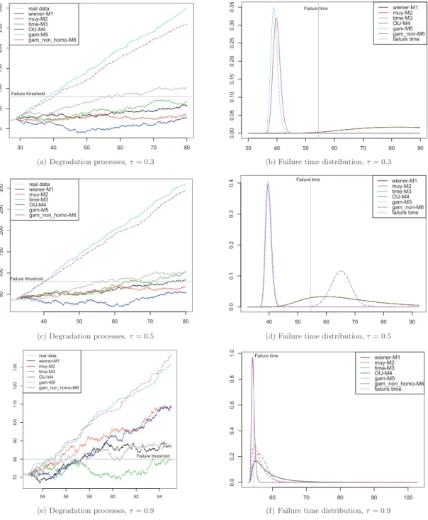
Fig. 3. Degradation processes generated (after parameter estimations from observation data generated by M 1 with 𝑣𝑐 𝑡 = 30% ) and failure time distributions estimated by models ( M 1 , ... M6 ) with different values of 𝜏.

Forexample,consider Table8that presents the results of model selectionaccordingtothePACandPHCwithdifferentvalueof𝜏for

datageneratedbyM₁ .When𝜏isincreasingfrom30%to90%,the

percentageofthechoiceofGammafamilyisincreasing,especially withhighvaluesofcoefficientofvariation.

Inordertoexplainthisparadoxresult,weconsideranexamplein whichdataaregeneratedbyM₁ withthecoefficientof variation 30%(seeFig.3).Basedontheobservationdatawithdifferentvalues ofthethreshold𝜏, theparametersof everymodelareestimated.

Then,thecorrespondingdegradationprocessesaregenerated(see

Fig.3(a),(c),(e)).TheircorrespondingRULdistributionsare esti-mated(seeFig.3(b),(d),(f)forestimatedfailuretimedistribution). When𝜏isincreasing(i.e.,formoregatheredobservationdata),the

RULdistributionsaremoreprecise.Whatevertheirshapesare,they aremore peaky,withalow varianceandcentered on theactual

failure time. Remark that this is mainly becausethe prognostic horizonisgettingshorter(i.e.,thelastobservationtimeiscloserto thefailuretime)asthevalueof𝜏increases.Eventhedegradation

processgeneratedbyGammamodels(M₅ orM₆ )giveresultswhich areclosetorealdataonashorttimepredictionhorizon.Itcanbe observed e.g.on Fig.3(f).The first passage times of degradation processes generatedby M₅ andM₆ areclose tothefailure time. ThenthefailuretimedistributionestimatedbyGammamodelsare themostaccuratecomparedtotherealfailuretime.Forashortterm horizon, these processes give good lifetime estimation with low variance.ThatisthereasonwhyaGammamodelcouldbechosen tobethebestmodelaccordingtoPACwhenmoremeasurements areobtained,andtheprognostichorizonisshort.

• Efficiency of the hybrid criterion: TheHyCthattakesintoaccount thegoodness-of-fitofobservationdataisthebestcriterionamong

Table 8

Model selection according to PAC and HyC with different thresholds of observed data generated by M 1 . vct Criteria M1 M2 M3 M4 M5 M6 (true model) 10% ( 𝑃 𝐴𝐶) 𝜏=30% 45% 17% 36% 2% 0 0 ( 𝐻𝑦𝐶) 𝜏=30% 39% 17% 41% 3% 0 0 ( 𝑃 𝐴𝐶) 𝜏=50% 37% 14% 30% 19% 0 0 ( 𝐻𝑦𝐶) 𝜏=50% 33% 16% 34% 17% 0 0 ( 𝑃 𝐴𝐶) 𝜏=70% 35% 21% 28% 16% 0 0 ( 𝐻𝑦𝐶) 𝜏=70% 34% 23% 27% 16% 0 0 ( 𝑃 𝐴𝐶) 𝜏=90% 21% 8% 25% 35% 5% 6% ( 𝐻𝑦𝐶) 𝜏=90% 25% 12% 29% 34% 0 0 30% ( 𝑃 𝐴𝐶) 𝜏=30% 26% 31% 36% 7% 0 0 ( 𝐻𝑦𝐶) 𝜏=30% 25% 33% 34% 8% 0 0 ( 𝑃 𝐴𝐶) 𝜏=50% 25% 22% 23% 30% 0 0 ( 𝐻𝑦𝐶) 𝜏=50% 20% 30% 21% 29% 0 0 ( 𝑃 𝐴𝐶) 𝜏=70% 11% 18% 16% 54% 1% 0 ( 𝐻𝑦𝐶) 𝜏=70% 13% 21% 16% 50% 0 0 ( 𝑃 𝐴𝐶) 𝜏=90% 2% 9% 3% 35% 26% 25% ( 𝐻𝑦𝐶) 𝜏=90% 3% 16% 13% 68% 0 0 50% ( 𝑃 𝐴𝐶) 𝜏=30% 21% 44% 27% 8% 0 0 ( 𝐻𝑦𝐶) 𝜏=30% 19% 51% 23% 7% 0 0 ( 𝑃 𝐴𝐶) 𝜏=50% 7% 33% 36% 23% 0 1% ( 𝐻𝑦𝐶) 𝜏=50% 9% 37% 32% 22% 0 0 ( 𝑃 𝐴𝐶) 𝜏=70% 4% 33% 20% 37% 4% 2% ( 𝐻𝑦𝐶) 𝜏=70% 3% 26% 23% 38% 0 0 ( 𝑃 𝐴𝐶) 𝜏=90% 1% 11% 3% 7% 44% 34% ( 𝐻𝑦𝐶) 𝜏=90% 1% 23% 18% 58% 0 0 70% ( 𝑃 𝐴𝐶) 𝜏=30% 14% 59% 22% 4% 0 1% ( 𝐻𝑦𝐶) 𝜏=30% 13% 64% 19% 4% 0 0 ( 𝑃 𝐴𝐶) 𝜏=50% 9% 60% 18% 8% 3% 2% ( 𝐻𝑦𝐶) 𝜏=50% 11% 62% 19% 8% 0 0 ( 𝑃 𝐴𝐶) 𝜏=70% 5% 37% 12% 8% 22% 16% ( 𝐻𝑦𝐶) 𝜏=70% 8% 56% 23% 13% 0 0 ( 𝑃 𝐴𝐶) 𝜏=90% 0 3% 0 2% 44% 51% ( 𝐻𝑦𝐶) 𝜏=90% 1% 46% 22% 31% 0 0

prognostic criteria. Infact,considerall theresultson Tables2–7. Based on HyC, the underlying model family (whether diffusion-based or Gamma-based processes) can be correctly identified in mostofthecases,evenifwhenthecoefficientofvariationishigh. Moreover, theparadoxresultdiscussedforPAC isalsobypassed. LookingforexampleatTable8,itcomesthattheunderlyingmodel familyiswellidentifiedwiththedifferent thresholdsof𝜏 evenif

thecoefficientofvariationishigh. 6. Conclusion

Inthispaper,wehavediscussedcharacteristicsofselectioncriteria fordegradation models.Theselectioncriteriaareclassified intotwo groups:(1)classicalstatisticalcriteriathatarebasedonthediscrepancy betweenobservationdegradationdataandthevaluesexpectedunder the considered model and(2) prognostic criteria that arebased on therelevancebetweenfailuretimeanditsexpecteddistributionunder the considered model. The advantages and disadvantages of these criteria are considered through numerous numerical examples for modelselectionbetweensolutionsofstochasticdifferentialequations andGammaprocesses.

Ingeneral,theclassiccriteriaisbetterthantheprognosticcriteria forthepurposeofdissociationofthetwofamilies(Gammavs. Brown-ian/OUmodels).Indetailamongclassicalcriteria,comparedtoEAL cri-terion,CVcriterionfavorsgeneralmodelswithhighparametersnumber whileAICandBICprefersasimplemodelhavingfewerparameters.As themodelcomplexityismorestronglypenalizedbyMDLcriterionwith thehypothesisofuniversalpriors,thenMDLcriterionfrequentlyfavorsa simplemodel.Hence,itisnecessarytoimprovetheformulationofMDL

bytakingintoaccountthepriorinformationaboutthedatadistribution andthemodelformality.Ontheotherhand,amongprognosticcriteria,

PHCistheworstcriteriatoidentifytheunderlyingmodelfamilyof ob-serveddata.Whenmodelparametersarewellestimated,theprognostic measureassessmentofeachmodelisapproximatelyequal.Considering

PAC,aninterestingparadoxresultisrecognized:thelongerthe obser-vationduration is,themorefrequently awrongunderlying modelis selected.Infact,whentheprognostic horizonis smallitmeansthat thelastobservationtimeisclosetothefailuretime.Thedegradation processgeneratedbyanothermodelcanbeclosetorealdataduringa shortperiodoftime.Therefore,itmaybecounterproductivetoincrease theobservationtimeforamodelselectionbasedonthePACcriterion. Thus,weproposednewcriteria,HyCthatallowstakingintoaccountthe goodness-of-fitofobservationdatawhenevaluatingtheprognostic mea-sures.NumericalexperimentshighlighttheperformanceofHyC. Partic-ularlytheunderlyingmodelfamilyofanobservationdataset,whether itisdiffusion(Brownian/OU)familyorGammafamily,canbecorrectly identifiedinmostofthecases,evenifthecoefficientofvariationishigh. Insummary,theclassicalstatisticalmethodsformodelcalibration arevery efficient.These methodsare usuallypowerful with alarge setof dataandthey donot take intoaccount thepossible posterior informationonthesystemoperationconditions.Theprognosticcriteria aremore strict andvery sensitivetothe coefficientfor variation of dataandthe decisionparameters. Moreover,these criteria aremore usefulwhentheoperationalconditionsaredifferentfromtheavailable trainingdegradationdata.Inthispaper,thesamedegradationdataare consideredforclassicalmodelselectionandprognosticcriteria. There-fore,theresults ofmodelselectionbringouttheinterestofclassical methods. Regardingthesensitivityoftheprognostic criteriaandthe precisionsoughtbythelatter,theyaremorerecommendedwhenthe operationalconditionsafterthelastobservationareveryfluctuating.

Theselectioncriteriapresentedinthispaperprimarilytakeaccount of the sampling errors in parameter estimation. Further works will considertheinfluenceofconfidenceintervalsofestimatedparameters on a model comparison. On the other hand, the impact of some characteristicfeaturesoftheobserveddatasetonmodelselectionwill beinvestigated,particularlysuchasthenecessaryamountofdata,the frequencyoftheobservations,periodicornot.Moreover,new appro-priate criteria that allow comparing parametric andnon-parametric modelsefficientlycouldbe developed.Thesetofmodelscanalsobe extended, andsome othermodelssuchas Variance-Gammaor jump diffusionmodelscanbeincluded.

References

[1] Liao CM , Tseng ST . Optimal design for step-stress accelerated degradation tests. IEEE Trans Reliab 2006;55(1):59–66 .

[2] Xu Z , Ji Y , Zhou D . Real-time reliability prediction for a dynamic system based on the hidden degradation process identification. IEEE Trans Reliab 2008;57(2):230–42 .

[3] Nikulin M , Limnios N , Balakrishnan N , Kahle W , Huber-Carol C . Advances in degradation modeling: applications to reliability, survival analysis, and finance. Birkhauser Boston; 2010 .

[4] Ye Z-S , Xie M . Stochastic modelling and analysis of degradation for highly reliable products. Appl Stochastic Models Bus Ind 2015;31:16–32 .

[5]Zhou RR , Serban N , Gebraeel N . Degradation modeling applied to residual lifetime prediction using functional data analysis. Ann Appl Stat 2011;5(2B):1586–610 .

[6]Kaipo J , Somersalo E . Statistical and computational inverse problems, theory and methods for parameter estimation. New York: Springer; 2005 .

[7]Muller H , Zhang Y . Time-varying functional regression for predicting remaining life- time distributions from longitudinal trajectories. Biometrics 2005;61:1064–75 .

[8]Bousquet N , Fouladirad M , Grall A , Paroissin C . Bayesian gamma processes for opti- mizing condition-based maintenance under uncertainty. Appl Stochastic Models Bus Ind 2015;31(3):360–79 .

[9]Bertoin J . Lévy processes, vol. 121. Cambridge University Press; 1998 . Part of Cam- bridge Tracts in Mathematics.

[10]Peng R , Li Y , Zhang W , Hu Q . Testing effort dependent software reliability model for imperfect debugging process considering both detection and correction. Reliab Eng Syst Saf 2014;126:37–43 .

[11]Peng R , Zhai Q . Modeling of software fault detection and correction processes with fault dependency. Eksploatacja i Niezawodnosc Maint Reliab 2017;19(3):467–75 .

[12]van Noortwijk JM . A survey of the application of gamma processes in maintenance. Reliab Eng Syst Saf 2009(1):2–21 .

[13]Lorton A , Fouladirad M , Grall A . Computation of remaining useful life on a physic-based model and impact of a prognosis on the maintenance process. J Risk Reliab 2013;227:434–49 .