Suspended sediment delivery from small catchments to the Bay of Biscay. What are the controlling factors?

Open Archive TOULOUSE Archive Ouverte (OATAO)

OATAO is an open access repository that collects the work of Toulouse researchers and

makes it freely available over the web where possible.

This is an author-deposited version published in :

http://oatao.univ-toulouse.fr/

Eprints ID : 16604

To link to this article : DOI :

10.1002/esp.3957

URL :

http://dx.doi.org/10.1002/esp.3957

To cite this version :

Zabaleta, Ane and Antiguedad, Inaki and

Barrio, Irantzu and Probst, Jean-Luc Suspended sediment delivery

from small catchments to the Bay of Biscay. What are the

controlling factors ? (2016) Earth Surface Processes and

Landforms, vol.41, n°13, pp. 1813-2004. ISSN 1096-9837

Any correspondence concerning this service should be sent to the repository

administrator:

staff-oatao@listes-diff.inp-toulouse.fr

Suspended sediment delivery from small

catchments to the Bay of Biscay. What are the

controlling factors?

Ane Zabaleta,1* liiaki Antiguedad,1 lrantzu Barrio2 and Jean-Luc Probst3 1

Hydrology and Environment Group, Science and Technology Faculty, University of the Basque Country UPV/EHU, Leioa, Basque Country, Spain

2

Department of Applied Mathematics, Statistics and Operations Research, Science and Technology Faculty, University of the Basque Country UPV/EHU, Leioa, Basque Country, Spain

3

EcoLab, University of Toulouse, CNRS, INPT, UPS, Toulouse, France

*Correspondence to: Ane Zabaleta, Hydrology and Environment Group, Science and Technology Faculty, University of the Basque Country UPV/EHU, 48940 Leioa, Basque Country, Spain. E-mail: ane.zabaleta@ehu.es

ABSTRACT: The transport and yield of suspended sediment (SS) in catchments all over the world have long been tapies of great interest. This paper addresses the scarcity of information on SS delivery and its environmental contrais in small catchments, espe-cially in the Atlantic region. Five steep catchments in Gipuzkoa (Basque Country) with areas between 56 and 796 km2 that drain into the Bay of Biscay were continuously monitored for precipitation, discharge and suspended sediment concentration (SSC) in their out-lets from 2006 to 2013. Environmental characteristics such as elevation, slope, land-use, soil depth and erodibility of the lithology were also calculated. The analysis included consideration of uncertainties in the SSC calibration models in the final suspended sed-iment yield (SSY) estimations. The total delivery of sedsed-iments from the catchments into the Bay of Biscay and its standard deviation was 272 200 ±38 107tyr.-1, or 151 ±21 tkm-2 yr.-1, and the SSYs ranged from 46± 0.48 to 217±106tkm-2 yr.-1• Hydroclimatic variables and catchment areas do not explain the spatial variability found in SSY, whereas land-use (especially non-native planta-tions) and management (human impacts) appear to be the main factors that contrai this variability. Obtaining long-term measure-ments on sediment delivery would allow for the effects of environmental and human induced changes on SS fluxes to be better detected. However, the data provided in this paper offer valuable and quantitative information that will enable decision-makers to make more informed decisions on land management while considering the effects of the delivery of SS. Copyright© 2016 John Wiley & Sons, Ltd.

KEYWORDS: suspended sediment yield; continuous monitoring; propagation of uncertainty; environmental contrai; Atlantic environment

Introduction

Rivers constitute the main linkage between terrestrial and marine systems (Knighton, 1998; Walling, 2006). The transport and yield of suspended sediment (SS) in catchments all over the world have long been tapies of great interest (Schumm, 1977; Mill iman and Syvitski, 1992; Farnsworth and Milliman, 2003; Milliman and Farnsworth, 2013) due to their raie in the global denudation cycle (Wald and Hay, 1990; Harrison, 1994), their importance to global geochemical cycling (Ludwig et al., 1996) and their potential raie as a pathway for the transport of nutrients (Walling

et al., 2001) and pollutants, including heavy metals (Ankers et al.,

2003) and micro-organisms (House

et

al., 1997). SS is essential for rivers because its presence or absence determines the geomorphological and biological processes that occur in these environments (Wass and Leeks, 1999).

Attempts to quantify SS fluxes from terrestrial to marine systems face a number of important problems, including the availability and reliability of data on sediment loads for rivers

(Walling, 2006). Despite these sources of uncertainty, some authors (Holeman, 1967; Mill iman and Meade, 1983; Mill iman and Syvitski, 1992; Ludwig and Probst, 1996, 1998, Milliman and Farnsworth, 2013) have been able to estimate that each year between 15 and 19 x 109 t of SS is delivered into the world's oceans by rivers. Recently, a global annual sediment yield of 190tkm-2yr.-1 was calculated by Milliman and Farnsworth (2013). Nevertheless, the global distribution of SS delivery rates is not homogeneous, and regional differences are considerable. ln Europe, for instance, whereas an annual yield of less than 10tkm-2yr.-1 has been calculated for northern rivers, the rivers that drain into the Mediterranean Sea have annual sediment yields that are one or two orders of magnitude higher (Vanmaercke

et

al., 2011; Milliman and Farnsworth, 2013). The same can be observed in Africa, where suspended sediment yields (SSYs) range from less than 10 t km-2 yr.-1 for the Senegal River basin (Kattan et al., 1987) in West Africa to more than 500tkm-2yr.-1 in the Maghreb area (Probst and Amiotte-Suchet, 1992). Vanmaercke

et

al.

(2014) explained that those differences found in SSYs in Africa are significantly correlated to tree cover and runoff.

A recent review by Garcia-Ruiz et al. (2013) showed that soil erosion and sediment transport have been intensively studied in Spain during recent years, and a total of 380 studies have been published in SCI journals. However, most of these studies have focused on the Mediterranean region, and publications about this topic in the Cantabrian basin are scarce. This publi-cation record reflects to the high density of SS data for the Mediterranean region of Spain, and the scarcity of data for the Atlantic region (including the Bay of Biscay) (Vanmaercke et al.,

2011 ). The first data on SS delivery to the Bay of Biscay were published by Uriarte (1998) and Maneux et al. (1999). Uriarte (1998) calculated that between 45 and 260tkm-2yr.-1 was transported to the coastal ocean from small catchments (drain-age areas between 40 and 780 km2) located in Gipuzkoa (Basque Country), whereas Maneux

et

al. (1999) estimated a SSY of 70 t km-2 yr.-1 for the Nivelle River (238 km2, French Basque Country). The latter highlighted the large contribution of small mountainous catchments, of basins smaller than 1000 km2 in size, to the total SS that were delivered to the Bay of Biscay because they transport more than the 50% of the total sediments that reach the coast.

lndeed, the key role played by small mountainous catchments in the delivery of SS to the oœan has been widely discussed (Mil liman and Syvitski, 1992; Leithold

et

al., 2006; Syvitski and Milliman, 2007). Approximately 45% of the total global sediment is delivered to the ocean from small ca.tchments. However, the database constructed by Vanmaercke

et

al. (2011) for European catchments revealed that relatively little data on SSY exists for

b)

Lithology

D Quaternary deposits

D Sandstones, shales and conglomerates

D Shales and siltstones D Marls El Stratified limestones D Massive limestones • Dolomites c 0 ·:: _g .ë. ·~ p.. • Volcanics • otites 2300 2000 1700 1400 1100 900 D Clays with gypsum D S!ates • Granites (fine grained) D Granites ( coarse grained)

• Granodiorites

small catchment:s. Furthermore, as Milliman and Farnsworth (2013) noted, there is a need to revise the estimates made for this type of catchment in global studies, considering that the number ofsmall mountainous catchments that have been monitored for a relatively long period is rather small.

The Department of Land Planning and Environment of the Gipuzkoa Provincial Council established gauging stations during the 1980s to record discharge data in catchments throughout its territory. From the 2000s, SS was sampled, from 2006 for rivers draining into the Bay of Biscay. The objective of the present study was to estimate the SS delivery from coastal small catchments (with areas smaller than 1000 km2) to the Bay of Biscay using existing high-resolution data. These data will enable the global SSY database ta be extended in a barely studied area and will offer new regional data that may be of interest to the scientific community working on denudation rates and sediment loads to the ocean, especially from small coastal catchments. Additionally, the data provide insight into environmental controls on the spatial variability found in SS delivery in Atlantic coastal environments.

Study

Area

The studied catchments are located in the province of Gipuzkoa, which is in the north-eastern part of the Basque Country (south-western Europe) and which has an average lat-itude of 43° and average longlat-itude of 1° (Figure 1 ). Gipuzkoa is a small province covering an area of approximately 1980 krn2. The altitude ranges from sea level to a maximum elevation of

d) 1600 Ê - 1300 ';;' 1000

.,,,

₇₀₀ .ê 400 ~ 300 - 200 <3 ~ 3-10 ';;;• 10-20 8..• 20-30 ..2

Cil

-

-

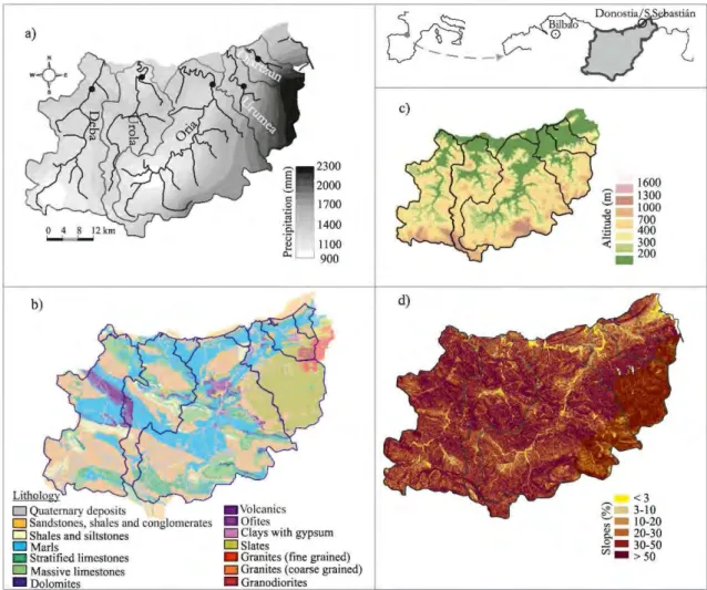
30-50 >50

Figure 1. Location and environmental characteristics of the studied area. (a) Studied catchments and the locations of the gauging stations (black

1554 m, and although the mountains are not very high, their slopes are steep and exceed 25% throughout most of the terri-tory, with average values between 40 and 50% for most of the catchments. The region is characterized by a humid and temperate Atlantic climate with 1500 mm of annual average precipitation (the precipitation is almost evenly distributed in all seasons) and a mean an nuai temperature of 13 °C that varies little between winter (8-10 °C, on average) and summer (18-20 °C, on average). A high spatial gradient is observed in annual precipitation; the maximums are registered in the east-ern part and decrease towards the west and the south.

Geologically, Gipuzkoa is located at the western end of the Pyrenees; the region is structurally complex and lithologically very diverse, with materials from Palaeozoic plutonic rocks to Quaternary sediments (EVE, 1990). Nevertheless, most of the materials in this region are sandstones, shales, limestones and maris, except in the eastern part of the region, where slates are predominant (Figure 1 b).

Forest is the predominant land-use in the area, and although autochthonous tree species have been promoted in recent years, pine tree plantations for timber production were introduced throughout the region in previous decades. With the government's promotion of afforestation policies in the second half of the twentieth century (Ruiz Urrestarazu, 1999), plantations with rapidly growing exotic species (primarily Pinus radiata) now caver 39-48% of potential native forestland on mountainsides and in areas with eleva-tions below 700-750 m above sea level (a.s.I.), respectively (Garmendia et al., 2012). Pinus radiata is very well adapted to the humid and temperate environment of Gipuzkoa, which allows large monoculture plantations to produce timber very efficiently (Michel, 2006). Forest management in these plantations involves clear-cutting on rotations of 30 to 40years along with mechanical site preparation for reforestation (i.e. scalping and down-slope ripping). Exotic species do not always fit local ecosystems perfectly, which can generate uneven extents of forest caver with small areas of bare soil exposed to direct rainfall. ln this respect, Porto

et al. (2011) found that in southern ltaly, the major contribu-tion of soil erosion could be ascribed to those small areas not covered by vegetation. ln contrast, Pinus radiata in Gipuzkoa are well adapted to the environment and have been considered rapid builders of forest communities (Carrascal, 1986; Ainz, 2008). Consequently, cutting and site preparation are the main drivers of land disturbance and sediment availability throughout the exotic tree planta-tions in Gipuzkoa. Additional human impacts on this region include civil engineering projects, for example, the con-struction of new highways and railways that can serve as important sources of river sediment. The effect of infrastruc-ture construction on the generation and source variability of sediments has been assessed by several studies (Rijsdijk

et al., 2007; Wu et al., 2012). A more recent publication (Martinez-Santos et al., 2015) showed the effect of highway tunnel construction on sediments in one of the catchments analysed in the present paper (Deba catchment).

Catchment characteristics

From west to east, five rivers, the Deba, Urola, Oria, Urumea and Oiartzun, drain the catchments that were analysed (Table 1). ln this study, the outlet of each catch-ment was considered to be the location of the last gauging station before the river discharges into the Bay of Biscay. Considering those outlets, the catchments drain a total area

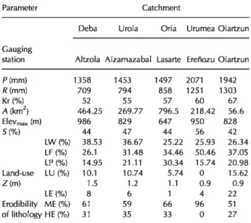
Table 1. Names of the gauging stations where discharge and SSC data for this research work were recorded. An nuai mean precipitation (P), runoff (R) and runoff coefficient (Kr) for the period 2006-2013 in the studied catchments. Area (A), maximum elevation (Elevmax), mean slope (5), land use (LW= exotic plantation, LF =native forest, LP = pasture, LU= others), mean soil depth (Z) and erodibility of lithology (LE= low erodibility, ME= medium erodibility, HE= high erodibility) for those catchments were also included. Source of data: (httpi/urhweb.gipuzkoa.net/)

Parameter Catch ment

Deba Urola Oria Urumea Oiartzun

Gauging

station Altzola Aizarnazabal Lasarte Ereîiozu Oiartzun

P(mm) 1358 1453 1497 2071 1942 R(mm) 709 794 858 1251 1303 Kr(%) 52 55 57 60 67 A(km2) 464.25 269.77 796.5 218.42 56.6 Elevmax (m) 986 829 647 950 828 5(%) 44 47 44 56 42 LW(%) 38.53 36.67 25.22 25.93 26.34 LF (%) 26.1 31.48 34.46 50.46 37.05 LP(%) 14.95 21.11 30.34 15.74 20.98 Land-use LU(%) 10.1 10.74 5.74 0 15.62 Z(m) 1.5 1.2 1.1 0.9 0.9 LE(%) 8 6 4 22 Erodibility ME (%) 61 59 66 96 51 of lithology HE (%) 31 35 33 0 27

of 1805 km2• The annual precipitation (P, in mm yr.-1) is spatially quite variable (Figure 1 a and Table 1) because more precipitation is recorded in the eastern part of the province (> 2000 mm in the Urumea and Oiartzun catchments) than in the middle and the west (< 1500 mm in the Deba, Urola and Oria catchments). The total runoff (R, in mm·yC\ which was calculated from the data recorded at the gauging stations, and the runoff coefficient (Kr, in %), which was estimated as the ratio between the annual runoff and annual precipitation as a percentage, show the same spatial pattern as the precipitation. Differences in the drainage areas (A) for each of the catchments are also important; Oria has the largest drainage area (796 km2), and Oiartzun has the smallest (56 km2).

The average slopes (5, %) calculated for the five catchments are very high and show, in general, slight differences; Urumea is the steepest catch ment (Figure 1 c and Table 1). Regarding land-use and vegetation, the Deba and Urola catchments have higher percentages of exotic plantations (LW), which are primarily Pinus radiata. Urumea has more native forests (LF), which are primarily beech and oaks, and the Oria catchment has the highest percentage of pasture (LP) (Table 1). Regarding land occupation, the catchments that are located in the middle and western part of the study area (Deba, Urola and Oria) suffer from the greatest human impact; they have larger population densities (maximums of more than 1000 inhabitants km-2 in contrast to the maximum of 150 in habitants km-2 in the eastern part of Gipuzkoa) and infrastructure construction pressures (primarily new motorways and high-speed railways).

The Urumea and Oiartzun have the smallest average regolith thickness (Z, in metres), and Deba has the thickest regolith (Table 1). The erodibility of the lithology was also considered a primary factor that may contrai the delivery of sediment. Following the classification proposed by Probst and Amiotte-Suchet (1992), which only considers rock hard-ness and sensitivity of lithology to mechanical erosion, on the basis of the data of Charley et al. (1984), granites and volcanic rocks were considered to be lowly erodible (LE);

maris, quaternary deposits and lutites with gypsum were classified as highly erodible (HE); and other lithologies, including sandstones, shales, limestones, slates and conglomerates, were considered to be lithologies with medium erodibility (ME) (Figure 1 b and Table 1).

Materials and Methods

Data acquisition and processing

Since October 2006, precipitation (in millimetres), water depth (in metres) and suspended sediment concentration (SSCF, in mg 1-1) have been measured in the field every 10minutes atthe gauging stations located at the outlets of each of the catchments. The gauging stations are included in the official hydro-meteorological network of the Basque Country. Discharge (in 1 Ç 1) is estimated from water depth through an exhaustive calibration conducted by the local hydraulic authorities of a water pressure probe installed in crump-type gauging stations (http://www4.gipuzkoa.net/oohh/web/esp/index.asp). ln the gauging station sections, direct discharge measurements are per-formed periodically and with higher frequency during extraordi-nary flood events. Three polynomial equations (for low, medium and high waters) relate pressure probe measurements of water depth and manual measurements of discharge for each station. The estimation error in discharge for those equations is between 0.1% and 0.8% (p=0.01) for low discharges, between 0.6% and 3.9% (p=0.1) for medium discharges and between 1.7% and 3.3% (p=0.1) for high discharges. SSCF is measured opti-cally using SOLITAX infrared backscattering probes (Dr Lange devices), with an expected range ofO to 10 000mg1-1• Addition-ally, automatic water samplers were also installed at the stations. The samplers were programmed to start taking the first of 24 samples of 800 ml of water when an increase in SSCF above 1 OO mg 1-1 was detected. Time interval between samples varies depending on the type of event expected in order to ensure that samples are taken in the increasing and decreasing limbs of the hydrograph and the sedimentograph. The samples are carried to the laboratory for physical suspended sediment concentration (SSCd measurements to calibrate the SSC measured by the probes in the field (SSCF). SSCL is measured in the laboratory by filtration of the samples through previously weighted 0.45-µm filters and subsequent drying and weighting.

The calibration of SSCF using physically measured SSC in the water samples is necessary in the catchments because the linear correlations (Pearson's r) between the instantaneous discharge and SSCF in each of the five catchments have been found to be rather weak (r= 0.58 in Deba;

r=

0.17 in Urola;

r=

0.59 in Oria;

r=

0.39 in Urumea;

r=

0.28 in Oiartzun) although statistically significant at the 1 % due to the large amount of data involved in the analysis (more than 300 000 data for each river). Even in Deba and Oria, where the linear correla-tions are stronger, a high degree of scattering exists (Figure 2). The scattering may be related to the high variability in SSC with dis-charge (hysteresis effects) due to variations in sediment availabil-ity and/or in the sources of sediments during different flood events. Due to these effects, sediment rating curves that relate SSCF to discharge are not suitable for use for sedimentflux predic-tions in these catchments.

For that reason, to estimate SS delivery from the catchments, the relationship between SSCF (measured continuously with the probe) and SSCL (determined from the samples collected by the automatic water samplers) was used to derive calibrated continuous SSC (in mg 1-1) data. These relationships are site specific; therefore, the relationships are typically unique for a particular catchment and sometimes within a particular period

of time (Gippel, 1989). Due to that specificity, in this study, a particular calibration was established for each catchment considering all of the events in which a threshold SSCF value of 100mg1-1 was exceeded. SSC values higherthan 100mg1-1 account for 5% of the values in Deba, 3% of those in Urola and Oria, 0.5% of those in Urumea and 2% of those in Oiartzun.

SSC calibration methodology

The relationship between SSCF and SSCL was investigated using generalized additive models (GAMs) (Hastie and Tibshirani, 1990; Wood, 2006). This type of method does not require any assumption of linearity between the predictor (SSCF) and response variable (SSCd, thus allowing the relation-ship between predictor and outcome to be modelled more appropriately. Smooth functions were estimated by means of P-spline smoothers (Eilers and Marx, 1996), which the literature suggests as the most convenient estimation technique (Rice and Wu, 2001 ). To fulfil the hypothesis of normality of the residuals, the response variable was log-transformed in those data sets in which it was required, such as Deba and Oria.

Suspended sediment load (SSL) and its temporal

variability

Once the calibrations and 95% confidence intervals for SSCF were established for each catchment (SSCunf, for the lowest and SSCL_sup for the highest boundary), annual suspended sed-iment loads (SSLs, in tonnes) were calculated using 10-minute SSCF measurements. For each 10-minute measurement, estima-tion of the SSCL was computed based on the estimated GAM and its confidence intervals. To allow full propagation of uncer-tainty associated with the SSCF-SSCL relationship, the SSLs were determined considering the 95% confidence interval of the estimated SSCL. A SSCL value was randomly selected in the 95% confidence interval of each prediction of SSCL, trans-formed from logarithmic to real space (where necessary) and multiplied by the corresponding discharge. This process was undertaken for each 10-minute interval within the selected time period (event, month, hydrological year) and repeated 2000 times for each gauging station. To this end, the following equation was used (Equation 1 ),

(1)

where SSCub is the instantaneous suspended sediment concentra-tion randomly selected in the interval (SSCunf,. SSCL_sup),

Q

is the instantaneous discharge, time is the 10-minute interval over which data were recorded at the gauging station, and SSb is the es-timated annual load in each b= 1, ... , 2000 replicates. This proce-dure permitted the derivation of basic statistical parameters [mean and standard deviation (SD)] for SSLs, based on the distribution of the 2000 replicates and the consideration of uncertainties inher-ent to the SSC calibration curves in the estimated SSLs.

The maximum SSCF value (data recorded by the field probe) accompanied by an SSCL value (data obtained in the laboratory by filtration and weighting of a water sample) is exceeded less than 0.07% of the time in Deba, 0.5% of the time in Urola and 0.02%, 0.007% and 0.05% of the time in Oria, Urumea and Oiartzun, respectively. The SSCL for those SSCF values above the maximum accompanied by physical data were estimated by extrapolating the trends of the GAMs, with standard errors set as identical to the running mean error calculated for the maximum observed SSCF (Tarras-Wahlberg and Lane, 2003).

3500 _cc

a)

_~

3000 • 2/18/2007 • 611012007 • 5/2412008 0 61112008 2500 ~ 0 611612008 • 9/1812009 • 3/1612011 ~2000 g ~ 1500

"'

1000 500 50 100 150 200 Q(m>/s) 2500 )

c

•

11/22/2006 • 11/1512007 2000 ~ 1500 5 • 1127/2009 • 111512011

...

0 1/1512013 250 300 3500

b)

3000

n

'

2500

.

~ 2000

..

g

..

~ 1500

•t

"'

1000 500 50 5000 4500

d)

4000 3500 ~3000 g 8 ,$ 2500 u 0 ~ i:l 2000

.

1500 1000 500 0 100 • 11/10/2009 0 11/26/2009 • 09/03/2011 • 1115/2011 01/15/2013 •5/1812013 =: ~: ~. o, ~:

.

" 100 150 200 Q(m3_/s) 100 Q(rn'is) 150 200 250 • 5/19/2008 • 0211212009 • 11/512011 • 11/28/2012 0 1115/2013 • 5/1812013 =:

.

.

O•

.

'

.:.:

.=...:

:=:

~l

r-:

+ ...

='*"

c

.

.

.

.

.

.

.

..

_.

_i

~

i

..

..._..._

.

_

_

...

_

...

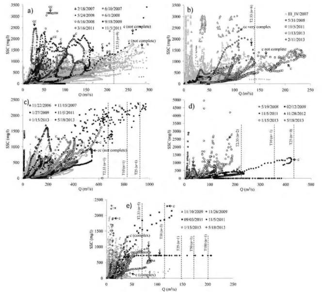
200 300 400 500 Q(rn3/s) 250

Figure 2. Suspended sediment concentration (SSC) versus discharge (Q) relationship for each catchment for the period 2006-2013. The major

events in each catchment are indicated by different symbols. c: Clockwise hysteresis; cc: counter-clockwise hysteresis. (a) Deba; (b) Urola; (c) Oria; (d) Urumea; (e) Oiartzun. Return periods (T2.33, T10, T25) for discharge along with the number of events that exceed each of those periods were indicated for each catchment.

The reportecl data represent measu rements taken 10-20 km upstream from the river mouth. Secliment is certainly depositecl downstream of the gauging stations, and new secliment is possi-bly i ntroducecl such that the reported sed iment load may not rep-resent the actual amount of sediment transported towards the ocean; however, the reported secliment is an approximation of the actual amount

of

sediment. Considering the results obtained at each gauging station and the calculated area for each catch-ment, an approximation of the SS yield from Gipuzkoa to the Bay of Biscay was also made using a weightecl mean.

Additionally, the temporal variability of SS was analysed using the Ts503 indicator (Meybeck

et

al., 2003), which corresponds to

the percentage of time necessary to carry 50% of the SS fi ux to the ocean. The Ts80% of the suspendecl sediment flux was also calcu-lated as in Delmru;

et al.

(2012). These indicators were calculatecl for the entire study period using the mean of the daily SSL data that had been previously obtained. The same indicators were calculatecl for the runoff (Tw₅₀₃ and Tw6CJ%).

Environmental controls on suspended sediment

yield (SSY)

Analyses of the effect of various hydrodimatic, geomorpholog-ical and lithologgeomorpholog-ical parameters related

to

the drainage basin of

each of the studied catchments on the mean of the SSL were undertaken. The considerecl parameters were selected based on availability of data for the five studied catchments. Besides this, it was intended

to

indude variables that are most widely reportecl to be related

to

soil erosion and sediment transport processes (Ludwig and Probst, 1998; de Vente

et al.,

2011) and show some variations in the studied region. Variables related to channel morphology were not included because, considering the small size of catchments, there are not impor-tant morphological variations between catchments that would imply significant differences in the SSYat the multiannual time-scale. Parameters that were considerecl and the corresponding data sets are listed in Table 1.

The hydrodimatic parameters that were induded in the anal-yses were the mean annual precipitation (P, in millimetres), mean annual runoff (R, in millimetres) and mean annual runoff coefficient (Kr, %) for the period 2006-2013. The precipitations were calculated for the entire catchment considering 48 mete-orological stations for the 1805 km2 of Gipuzkoa Province.

The other geomorphic parameters that were considered in the analyses were the area of the catchment (A, in km2), maxi-mum elevation (Elevmaxr in metres), mean slope (S,

%),

the average soil depth (Z, in metres) and land-use as a percentage of exotic plantation (LW, %), native forest (LF, %), pasture, including cultivated land (LP, %), and other uses, including

urban, artificial, water bodies, bare rock (LU,%) in the catch-ment. ln this region, cultivated land is considered together with pasturelands because in Gipuzkoa the percentage of crop cul-tivated area is very low and it is distributed in small lands that do not have the environmental impact of wide agricultural areas. ln fact, the main cultivated areas of Gipuzkoa are exotic plantations. The erodibility of rock was also considered as the percentage of the catchment with lithologies that had low (LE), medium (ME) or high (HE) erodibility. Ali the data were derived from geographic information system (GIS) data that are freely available at the Department of Land Planning and Environment of the Gipuzkoa Provincial Council (http:// urhweb.gipuzkoa.net/, accessed 12 January 2015) and Basque Government (www.geoeuskadi.net, accessed 12 January 2015) websites.

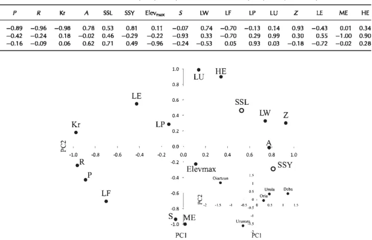
The relationships between ail of the variables and the means of the SSY and SSL were assessed. First, the relations between the hydroclimatic, geomorphic and lithologie parameters with SS were assessed using linear correlations (Spearman correla-tion coefficient and its significance level). Later, principal com-ponent analysis (PCA) was completed to assess the main factors that contrai the spatial variability of the SSY in the studied region and describe the relationship between ail the variables. The PCA was performed with a Varimax rotation to better visu-alize the principal components (PCs). PCA was based on log-transformed data in order to normalize distributions.

Results

SSC versus discharge relationships

Figure 2 shows SSC and the discharge data that were recorded every 10 minute from 2006 to 2013 for each catch ment. ln the studied locations, the low percentage of missing values for discharge and SSC should be noted. There are no missing dis-charge values for any of the gauging stations, and the percent-ages of missing data for SSC are 0.11 % in Deba, 0.47% in Urola, 0.25% in Oria, 0.01 % in Urumea and 0.25% in Oiartzun. Most of these data are missing during high flow periods, which is when most instrument malfunctions happen. However, we consider the minimal number of gaps and the length of the series to provide sufficient confidence to the obtained results. ln Figure 2, even if SSC seems to increase with increasing discharge, a large amount of scattering in the rela-tionship between the instantaneous SSC and

Q

measurements can be clearly observed. Such scattering may be related to variations in sediment availability according to the season, hydrological characteristics and/or source of different events contributing sediment. As a consequence, such variations would induce hysteresis effects that could be observed in those relationships, particularly during flood events between rising discharge and recession periods (Williams, 1989; Lenzi and Marchi, 2000; Smith and Dragovich, 2009). Additionally, Figure 2 shows the major events (concerning discharge, SSC or bath) registered for each site during the study period (between five and eight events) using different symbols. The lack of a global relationship between SSC and discharge for each river, along with different relationships between those parameters for different events in each of the analysed catch-ments, are also evident in Figure 2.

Most of the basins in Figure 2 follow a similar pattern - even if a general positive relationship exists between SSC and dis-charge, higher maximum concentrations of SS were detected in events with lower maximum discharges, and there was a decrease in the maximum SSC with an increase in maximum discharge. Therefore, during events with lower maximum

discharges, which were usually related to drier conditions (lower initial discharges), more intense precipitation (between 2 and 8 mm in 10 minute of maximum precipitation intensity) and higher surface runoff contribution, sediments were more concentrated. However, during wetter periods when precipita-tion lasts longer (2-3 days) and maximum discharge is higher, sediments are more diluted in water, but the total sediment amounts are usually higher. Nadal-Romero

et al.

(2015) found that Atlantic storms approaching from the northwest are the most influential precipitation events in the study region in terms of runoff and sediment yield. ln Oria, this pattern was not as clearly observed, and higher maximum discharges were appar-ently related to higher concentrations of SS. This trend may be related to higher surface runoff contribution combined with a higher capacity of water fluxes to transport more and/or coarser sediments.

For each of the events highlighted in Figure 2, the SSC regis-tered in the rising limb of the hydrograph is different from that registered in the falling limb, which shows a clear hysteresis effect that has been widely observed in other catchments (Kattan

et al.,

1987; Williams, 1989; Llorens

et al.,

1997; Alexandrov

et al.,

2003; Seeger

et al.,

2004; Rodriguez-Blanco

et al.,

2010). ln ail of the catchments, clockwise hysteresis loops can be observed between SSC and

Q

for most of the major events because the maximum concentration is registered before the maximum discharge and the SSC in the rising limb of the hydrograph is higher than in the falling limb. For such events, Probst (1986) and Etchanchu and Probst (1986) showed that the contribution of surface runoff to the total river dis-charge is higher during the rising period than during the falling limb of the hydrograph, and during the rising period, this con-tribution increases the mechanical erosion of the soils and the SSC in the river. Moreover, Kattan

et al.

(1987) proposed that the remobilization of bottom sediment deposited after a previ-ous event could contribute to an increase in the SSC during the rising period. Williams (1989) suggested a rapid depletion of the available sediment coming from a river channel before the runoff peak was reached. There are some cases in which the maximum SSC is reached after the discharge peak and the concentration of sediments is higher in the falling limb of the hydrograph than in the rising one, which produces a counter-clockwise hysteretic loop. ln the studied catchments this type of loop is usually observed during intense precipitation events that occur under dry soil moisture conditions. This type of loop has been explained by the presence of significant sources of sediment that are distant from the major runoff generation area (Williams, 1989; Brasington and Richards, 2000; Seeger

et al.,

2004).

Due to the high uncertainty related to the use of sediment rating curves in this case, to estimate the SSC in the river and SS delivery from the studied catchments, the relationship between SSCF and SSCL was used to derive calibrated contin-uous SSC (in mg 1-1) data for each catchment. Sixty-three events in Deba, 39 in Urola, 42 in Oria, 15 in Urumea and 21 in Oiartzun were analysed and included in the regressions. For the five catchments that were studied, SSCL was regressed against the corresponding SSCF values using a GAM. The calibrations and their 95% confidence intervals are presented in Figure 3.

Field-laboratory relationships (SSCF versus SSCLl can be ade-quately described for the Urola, Oria, Urumea and Oiartzun gauging stations (Figures 3b-3e) using unique models. The fact that regressions do not change throughout the studied period indicates that the physical properties of the suspended particles remain, on average, more or less constant for different events, even if there is a high diversity of lithologies in the catchments. However, changes in the physical characteristics (mainly size)

CO I'-c:o ...J () (/) lO (/) ~ v

"'

N 0 ...J 0 () CO Cf) Cf) 0

8

_lO

8

0 ü ~ Cf) Cf) 0 0 lO 0

a

.

l)

..

_...

0 500 0 500

d)

1000 SSCF 1000 SSCF n = 374 R2_{= 0.72} 1500 2000 1500

"

.

;:>

'..: : ... ·· -

~

;

~~

.

8

.. _,. p-value < 0.00 / 0 500 1000 1500 2000 2500 3000 SSCF

ü

(/) ~ lO 0 v N 0 ~

ü

Cf) _CO Cf) ~ c:o v N 0 0 0 ~ ...J 0

() g

Cf) Cf) 0 0 N 0

a.2)

,,,/' 0

c)

0

e)

0 ,,'/

_

... -

..

-··-~--

_.!

:. _____

__ ...

·

n =-;·~~ ···;~---

.

.. ,

_

_

__

R2 _{= 0.81 '\,_} p-value < 0.00 ',_ ~ ... ___ , 500 1000 1500 2000 2500 SSCF n = 368 R2 _{= 0.73} p-value < 0.00 1000 n=40 R2_=0.81 p-value < 0.00 2000 SSCF

,/'',

___

..

·'\

\

\ ~'

...

/ 3000 4000 200 400 600 800 1000 1200 1400 SSCF

Figure 3. Generalized additive models (GAMs) for field suspended sediment concentration (SSCF, in mg 1-1, optical) and laboratory suspended sed-iment concentration (SSCL, in mg 1-1) regressions with their 95% confidence intervals for (al) and (a2) Deba, (b) Urola, (c) Oria, (d) Urumea and (e) Oiartzun Rivers. Data from events registered from October 2006 to September 2013 are included in ail of the regressions. ln Deba two regressions are included: (al) for most of the 2006-2013 period; (a2} for the period between November 2011 and February 2012. See explanation in the text.

of SSs from event to event cannot be discounted, considering that the adjusted models are not simple linear regressions but are rather more complex models. Those changes in transported sediment size influence the relationship between the visual SSC measured in the field (SSCF) and the physical SSC measured in

the laboratory (SSCi) (Regüés et al., 2002). Finally, for the Deba

catchment (Figure 3a1 and 3a2), no unique relationship is observed throughout the study period. As suggested by Lewis (1996), calibrations for individual events were produced, and two data sets are distinguished in the graph. One of these uses most of the events that occurred in the Deba River and the other runs from November 2011 to February 2012. This second set of samples appeared as a consequence of the upstream remobilization of a large amount of previously accumulated organic matter during an extreme event in November 2011. Considering this change, a different GAM was applied for each of the studied periods in Deba.

Suspended sediment delivery to the ocean

Table Il presents the annual data for precipitation (P, in

millimetres), runoff (R, in millimetres) and suspended sediments

SSs, along with the means and SDs (SSL, in tonnes; SSY, in t

km-2) for the studied catchments. Approximately 172 600

±84 641 t·yr.-1 (i.e. 63% of the SSs delivered to the Bay of

Biscay from this region) was exported from the largest catch-ment, Oria (Figure 4a). The Deba River was second, with

almost 53 500±9B24tyr.-1, or 20% of total exported

sedi-ment. Together, the two largest rivers exported 83% of the SSs from 70% of the drained area. Urola exported approximately 31 700±84t (12%) and Urumea and Oiartzun exported 10

100 ± 106 and 4400 ± 2 0 t yr. -1

, respectively. Therefore, the

largest rivers exported more sediments than the smallest rivers. When drainage area was considered and the SSY was calculated, the Oria catchment had the highest mean SSY of

217±106tkm-2,

followed by

Urola, Deba, Oiartzun and Urumea,

with 117±0.31, 115±21, 78±0.35 and 46±0.48tkm-2,

respectively (Figure 4b). The differences observed in the SSY of the five catchments are explained later in this paper, when the environmental controls determining spatial variability of SS delivery are identified. Based on these calculations, the total delivery of sediments to the Bay of Biscay from Gipuzkoa

was estimated to be approximately 272 200±38 106tyr.-1

(i.e. 151 ±21 tkm-2yr.-1) for a total drainage basin area of

1805 km2•

ln general, uncertainty in SS delivery associated to SSCr SSCL relationships in these five catchments is rather low (Table Il). However, the Oria catchment shows a mean SD at 50% of the estimated SSY. This high mean uncertainty is due

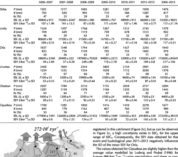
Table Il. Annual precipitation (P, mm), runoff (R, mm), nmoff coefficient (Kr, %), suspended sediment load (SSL, t) with its standard deviation (:1: SD) and suspended sedi ment yield (SSY, t·km -2) with its standard deviation (:!: SD) for the Deba, U roi a, Oria, U rumea and Oiartzun catchments between

2006 and 2013. ln the last column, the calculated mean annual precipitation, runoff and suspended sediment load and yield for the studied period

(2006-2013) are listed. P, R, Kr, SSL and SSY data for Gipuzkoa are also included. The precipitation presented in this table was estimated for the entire catchment, taking into account all of the rain gauges in the study area

2006-2007 2007-2008 2008-2009 2009--2010 2010-2011 2012-2013 2006-2013 Deba P(mm) 1501 1217 1693 1281 1207 1959 1476 R(mm) 705 640 995 710 566 1287 817 Kr(%) 47 53 59 55 47 66 55 SSL (t), :1: SD 49800:1:912 75000±6267 40300±380 48900±767 48900±912 66000±332 53500±9824 SSY (t km -2) ± SD 107±1.96 161 ±13.5 87±0.82 111 ± 0.64 107±1.96 142 ±0.71 115±21.16 Urola P(mm) 1526 1307 1768 1367 1312 2195 1579 R(mm) 709 649 1119 739 678 1515 902 Kr(%) 46 50 63 54 52 69 57 SSL (t), ± SD 80600±90 17200±52 21300±69 16700±73 12700±49 49200± 107 31700±84 SSY (t km -2) ± SD 299±0.33 64±0.19 79 ±0.26 62 ±0.27 47±0.18 182±0.39 117 ±0.31 Oria P(mm) 1657 1348 1764 1381 1427 2265 1640 R(mm) 833 754 1139 793 753 1602 979 Kr(%) 50 56 65 57 53 71 60 SSL (t), ± SD 38600±2260 29400±222 197600 ± 70328 94800±2215 52900±312 150200±637 172600 ±84641 SSY (t km -2) ± SD 48±2.84 37±0.28 248±88 119±2.78 66±0.39 189±0.8 217±106 Urumea P(mm) 2405 1844 2344 1805 2134 2991 2254 R(mm) 1224 1232 1554 1058 1172 2030 1378 Kr(%) 51 67 66 59 55 68 61 SSL (t), ± SD 7100±55 3200±52 10900±96 5300±50 9600±74 19000± 134 10100±106 SSY (t km -2) ± SD 33 ±0.25 15 ±0.24 50±0.44 24±0.23 44±0.34 87±0.61 46±0.48 Oiartzun P(mm) 2037 1784 2210 1745 2059 2727 2094 R(mm) 1297 1139 1578 1169 1255 2230 1445 Kr(%) 64 64 71 67 61 82 69 SSL (t), ± SD 1600±11 1200±9 5200±14 5200±24 5400±26 7500±23 4400±20 SSY (t km -2) ± SD 28±0.2 21 ±0.15 92 ±0.25 91 ±0.42 96±0.46 132±0.4 78 ±0.35 Gipuzkoa P(mm) 1700 1382 1830 1416 1459 2278 1677 R(mm) 843 779 1163 807 760 1579 989 Kr(%) 50 56 64 57 52 69 59 SSL (t), ± SD 177800±1091 126000±2804 275400±31452 1 70900 ± l 049 130500±433 291800±330 272200 ± 38107 SSY (t km -2) ± SD 98±0.6 70±1.55 154±17

Figure 4. An nuai discharge of suspended sediment (SS) fmm the

stud-ied catchments. The widths of the arrows correspond to the relative sediment loads. The colours of the catchments refer to the relative sed-iment yield. The numbers inside the arrows refer to the average annual sediment delivery in thousands of tonnes per year. The numbers inside each catchment refer to the suspended sediment yield in tonnes per square kilometre and year.

to the high range of values obtained in the 2000 replicates for

the hydrological year 2011-2012. During November of 2011, an extraordinary event with high discharge and SSCF data was

95±0.58 72 ±0.24 162 ±0.18 151 ±21.1

registered in this catch ment (Figure 2c), but as can be observed in Figure 3c, a high uncertainty exists in SSCL for the upper range of SSCF. Consequently, the SSY data obtained for that event and hydrological year 2011-2012 negatively influences the SD of the mean SSY for Oria.

The values obtained for Gipuzkoa are slightly higher than the average value modelled by Ludwig and Probst (1996) for

Europe (88tkm-2yr.-1) using precipitation and slope as

con-trolling factors, primarily due to the higher SSYvalues of catch-ments located in the middle and west of the study region (Oria, Urola and Deba). However, with the exception of the Oria catchment, these values are below the global annual sediment

yield of 190 t km-2 _{yr. -}1 _{calculated by Mi Ili man and}

Farnsworth (2013) and the 279tkm-2yr.-1 figure reported

by

Vanmaercke

et al.

(2011) as the mean value for European

catchments based on data gathered from gaugi ng stations. The values obtained in the present study are on the order of

the mean SSY of 1 OO t km-2 yr. -1 estimated for European

catch-ments located in the Atlantic climatic zone by Vanmaercke

et al.

(2011 ). However, the results of this study are quite high

compared with the sediment fluxes estimated by Delmâs

et al.

(2012) for the French rivers that flow into the Bay of Biscay, except for the case of the Urumea River. Using the lmproved rating curve approach (IRCA) method, the authors

calculated SSYs between 8 and 36tkm-2yr.-1 for the Loire,

Garonne, Aquitaine and Adour and Gaves zones, which have

catchments that are larger (> 1 0 000

km

2

) than those analysed

in the present study. Uriarte (1998) derived SSYs between 20

A. ZABALETA

regressions of SS against river discharge for discrete or daily integrated water samples. These values are higher than those estimated in the present study, which are based on continuous optical measurements and a higher sampling frequency. How-ever, Mill iman (2001) identified wide variations in the SS regimes of European rivers, which are related ta anthropogenic activity and other causes.

SSL and SSY estimations can be strongly influenced by the range of events within the measurement period (Regüés et al.,

2000; Lenzi and Marchi, 2000; Sun et al., 2001; Ferro and Porto 2012). Ta assess the effect of events of different frequency and magnitude in each of the catchments, return periods for each of the sites were included in Figure 2, along with the num-ber of events that exceeded a certain return period in each catchment. Return periods of 2.33, 10, 25, 50, 1 OO and 500years (URA, 2012) are considered in Figure 2.

ln Oeba, each of the nine events that exceeded the 2.33-year return period (T2.33) accounted for between the 10% and 70% of the an nuai SS delivery of that catchment for the hydrological year of occurrence. ln the Urola catchment, six events exceeded the 2.33-year return period, delivering between 25% and 55% of annual SSs. ln Oria, only one exceptional event was responsible for 90% of the SS del ivered ta the ocean during the hydrological year 2011-2012. This was a 25-year return period event (T25). ln Urumea, two events exceeded the established thresholds, with one T2.33 event accounting for almost 60% of SS delivery in one year and a Tl 0 event that delivered the 80% of annual SS in another. Finally, in Oiartzun, five events exceeded the 2.33-year return period, two exceeded Tl 0 and one exceeded Tl 00. Approximately 50% of the annual SS was delivered du ring this last event. The other four events (2 T2.33 and 2 Tl 0) were responsible for delivering between 20% and 35% of annual SS.

These data show the importance of low frequency events for SS delivery ta the ocean, as they account for a high percentage of total SS delivery for a single year. However, the amount of sediment delivered during those extraordinary events show a wide range, especially in Oeba and Urola catchments, where events of the same return period (T2.33) can deliver anywhere from a small percentage of annual SS ta more than the half of it. Conversely, in Oiartzun, events with different return periods (T2.33 and Tl 0) account for a similar percentage of the annual SS. Furthermore, catchments where events with higher return periods were recorded (Oiartzun, Urumea and Oria) are not necessarily those that show higher SS delivery rates. Therefore, other characteristics are also responsible for the amount of SS that an event can transport, which include antecedent condi-tions, precipitation amount and intensity, duration of the event or sediment availability, among others (Old et al., 2003; Nearing et al., 2005; Seeger et al., 2004; Zabaleta et al., 2007). Table Il also includes annual precipitation and runoff. A regional analysis of the hydrology in the Gipuzkoa territory (Zabaleta, 2008), in which 22 gauging and meteorological stations were analysed for more than 1 5 years, showed that a significant difference existed in the annual runoff coefficient between the catchments that are situated in the eastern part of the region and those in the western part. Therefore, a progres-sive decrease in precipitation and its productivity (in terms of runoft) from east ta west was detected. Based on the corre-sponding analysis and the data presented in Table Il, it can be observed that even if higher amounts of precipitation and runoff are registered for the catchments located in the east (Oiartzun and Urumea) than for the remaining catchments, the eastern catchments have the lowest calculated SSY. Based on these data, one could suspect that there must be other variables (that are not related ta hydroclimatic variables) that are major con-trais of SSY on a regional scale in this area.

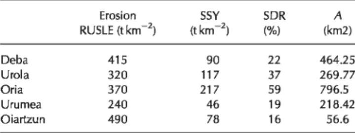
ln the relationship between sediment delivery and erosion (sediment delivery ratio, SOR), sediment storage is a key factor for better understanding the physical processes and geomorpho-logical evolution of the landscape. As demonstrated by Walling (1983), the SOR decreases when the drainage basin area increases. Porto et al. (2011) stated that the clear inverse trend be-tween catchment area and SOR found in southern ltaly largely reflected the increasing opportunity for sediment deposition and storage with larger catchment area. For the coterminous United States, Holeman (1980) calculated that only 10% of total eroded sediment reaches the ocean, and Wasson et al. (1996) es-timated that in Australia only 3% of the soil eroded in the external drainage basins is delivered ta the ocean. Nevertheless, in a semi-arid area such as southern Morocco, Haida et al. (1996) showed that SOR cou Id reach 67% in the Oued Tensiff drainage basin (18 400 km2). ln our case study, the official erosion estimates (Basque Government, 2005) made using the RUSLE equations were com-pared with the SSYs calculated in the present paper ta provide an order of magnitude estimate of the SOR (Table Ill), even if RUSLE is not perfectly adapted ta our regional conditions. Erosion rates and, consequently, derived SORs show important differences depending on the catchment. Considering the drainage basin area and relationships for different regions, the SORs obtained for Oeba, Urola, Lasarte, Urumea and Oiartzun, are in the range (16-59%) of those published by Walling (1983). However, they are higher than those calculated for catchments of more than 1000 km2 in Australia by Wasson et al. (1996) or for catchments between 1.47 ha and 31.61 km2 in southern ltaly by Porto et al.

(2011 ). The SORs calculated for Oeba and Oria are the highest in the studied area (37-59%). Small mountainous rivers generally have small flood plains and are more susceptible ta floods and it is assumed that less sediment is deposited in smaller drainage basins than in larger ones. However, in Gipuzkoa, the drainage basin area does not appear ta affect SOR because the highest SOR can be observed for the largest catchment and the lowest SOR for the smallest one. ln this sense, Walling (1983) and de Vente et al. (2011) emphasized the uncertainties with respect ta temporal and spatial aggregation of data on sediment transport, sediment yield and explanatory factors such as climate, land-use and lithology. We will return ta this point when discussing the temporal variability indices for SS.

Table Il shows the high variability of the SSLs from year-to-year, which is much higher than the variability in the precip-itation or runoff. The largest amount of SS, with associated larg-est uncertainty, was exported from Gipuzkoa in the 2011-2012 hydrological year, a total of 733 500 ± 95 735 t. However, 2011-2012 was not the rainiest year (the precipitation was below the mean of the study period for each catchment) nor the year with the highest total runoff (even if the total runoff exceeded the mean of the study period for each catchment), but the runoff coefficients calculated for year 2011-2012 were quite high and exceeded 60% for most of the catchments, as a consequence of an extreme runoff event (Figure 2).

Table Ill. Erosion estimates made using the RUSLE equation (Basque Government, 2005), mean SSY (this paper) and sediment delivery ratio (SOR) calculated from those data. The area (A, km2) of the

studied catchments is also included in the table

Erosion SSY SOR A

RUSLE (tkm-2) (tkm-2) (%) (km2) Oeba 415 90 22 464.25 Urola 320 117 37 269.77 Oria 370 217 59 796.5 Urumea 240 46 19 218.42 Oiartzun 490 78 16 56.6

Temporal variability of SS delivery

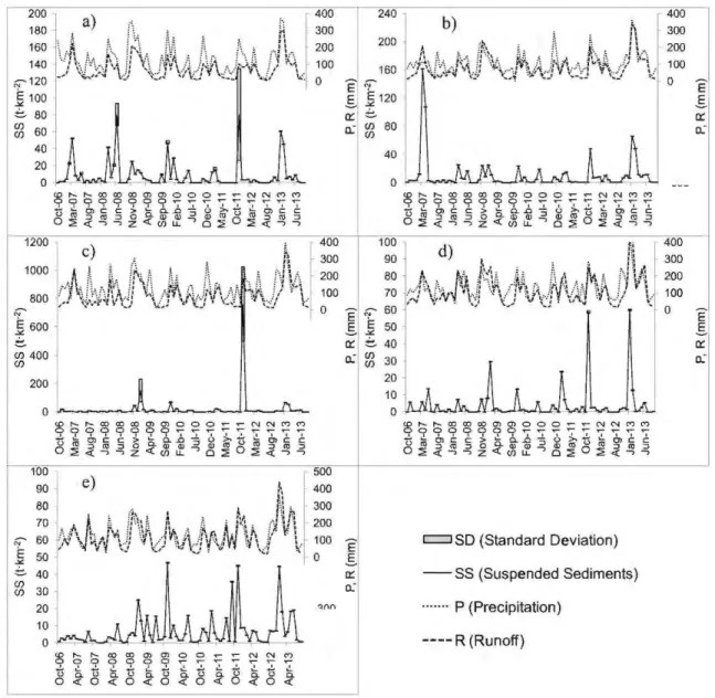
Figure 5 clearly shows that there were extraordinarily high deliveries of SS (cornpared with the rest of the data) during the spring of 2007 in the Urola catchment and during the auturnn of 2011 in the Oria cat.chrnent. The high SSLs caused 2006--2007 and 2011-2012 to

be

the years with the highest levels of SS export in Urola and Oria, respectively. ln Urola, this extrernely high output of SS occurred when a factory located approximately 20 rn upstrearn of the measurement station began excavation to expand its area. The excavated area had a volume of approxirnately 150 000 m3, which would account for 142 500t of material, assuming a soil density of 0.95 tm-3• Therefore, the excavation generated a large amount of SS that was available for transport and delivery out of the catchrnent. The anornalous increase in SS delivery in 2006--2007 was approximated using the regression between runoff (in millirnetres) and SS delivery (in t km-2) using monthly values (R2=0.74) for the period 2007-2013 (Figure 6a). The regres-sion between these two parameters improved from the 10-minute to monthly scale because hysteresis effects did not affect their relationship on the longer timescale. The regression was then applied

to

the runoff data observed over the period 2006--2007 to obtain theoretical SS delivery values from Urola under non-modified conditions (Figure 6b). The difference

1200 1000 800 N ~ 600 t:. (/) 400 (/)

c)

~

;j

\l:.

1~t

\~ij\td~\it

-lvv{\

·}AJf \

1

\

<.Ot--t--COCOO'.>ŒOO N N M 0 0 0 0 0 0 0 ~ ~

8~8~8~8~8.î8~8~

400 300 200 100 0 400 300 200 100 0 500 400 300 200 100 0 ~"" N

between the observed and the theoretical SS del ivery reached 235tkm-2, 63 500t or 60 300m3 (assuming a density of 0.95 t m-3), representing 78% of the SS delivered to the coastal ocean from the Urola cat.chment over the period 2006-2007. This supplementary sediment was transported during March and April and can be attributed to higher availability of SS derived from human impact in the catchrnent, which was to a great extent due

to

the previously mentioned excavation works. Therefore, in this case, the increase in SS cannot be associated with uncertainties in the calibration of SSC data, and although the SD of SSY is very low in this catchment, it was clearly pro-voked by human activity.

However, in November 2011, the SSL in the Oria River was at least four times higher than that of any other month (Figure 5), with a high uncertainty associated to the SSCr-SSCL regression model. This high SSL was generated as a consequenœ of an ex-trerne runoff event (the highest runoff registered, at least between 1999 and 2012). A lower-magnitude increase in discharge and SS delivery in November 2011 can also be identified forthe other catchments because the strong rainfall event was regional (Figure 2).

Following the previously mentioned approach, a regression between the monthly means of SS delivery (in t km-2) and run-off (in millimetres) was conducted for each of the five catch-ments to account for seasonal variations over the period

240 200 160

b)

~

/

~

/\

f~~J\\

Jl~

-\t"~:v~\AA\:~-

1

~\~~;

·

j t~\

i

400 300 200 100 0 E E ~ 120

.s

Ê a:: a.· (/) ₈₀ (/) 40 0 100 90 80 70 Ê ;::;-- 60 E E 50 ~ ~ O:'. t:. 40 o.: ~ 30 20 10 0 Ê

.s

a:: o.:

c::::::J SD (Standard Deviation)

- SS (Suspended Sediments) ··· P (Precipitation) ---- R (Runoff) 400 300 200 100 0 a:: o.: Ê

.s

O:'. a."

J

Figure 5. Monthly precipitation (P, in millimetres), runoff (R, in millimetres) and specific suspended sediment Joad (SSL) with its standard deviation (in t km-2) for the (a) Deba, (b) Urola, (c) Oria, (d) Urumea and (e) Oiartzun catchments for the period 2006-2013.

a) 200 180 160 N-140 ] 120 6100 (/) (/) 80 1:-. -5 60 Q

~

40 20 0 • uro la 2007-13 • uro la 2006-07

•

•

y= 0.0004x2_{+ 0.038x} R'= 0.82 n=72 p-value=0.000

.

~

.

.

. . .

A ' E f • • • • b) ~ N

i:

-"' .:::;, </} </} 180 160 • uro la observed 06-07 140 • uro la ù1eoretical 06-07 120 100 80 60 40 20 0

""

"" ""

r-- r-- r-- r-- r-- r-- r-- r-- r--0 0 0 _S' 0 0 0 0 0 _S' 0 0 0 100 200 monthly Runoff 300 400 .!. u

>

& c: J, 0

_"

_~

"'

.!. .!.

_>.

_C: ~

_""

o.

"'

o.

"'

.:::

_~

"'

0

_z

a

LI.. ₂ <!'. ₂ </}

Figure 6. (a) Monthly mean suspended sediment (SS, in t km-2) versus monthly runoff (in millimetres) for the Urola catchment over the periods

2006-2007 and 2007-2013. The regression for the period 2007-2013, with the number of data involved (n), the determination coefficient (If)

and the significance level of the regression (p-value) also induded. (b) Observed and theoretical SS delivery (in t km-2) from the Urola catchment over the period 2006-2007. The theoretical SS delivery was calcu lated usi ng the monthly relationsh ip between runoff (in mi 11 imetres) and SS delivery (in t km-2) from October 2007 to September 2013.

2006-2013 (Figure 7). For the regressions, a confidence inter-val of 95% was calculated. There was no significant hysteresis on the monthly timescale, and the regressions that are shown

;::;--160 140 120 ;:: 100 .l2 ~ 80 </}

a)

y= 9· J0_R'·5₌ x_0.57 2+ O. 115x n=84 p-value=0.000 ;... 60 "

~

40

~

~

E 20 e

e

~

-0

~

----=-~---0 50 1200

c

)

1000

fsoo

.:;< 6600 </} Vl ~400 c: 0 E 200 0 0 50 1 OO 150 200 250 300 350 100 monthly Runoff (mm)

j

y= 1 ·I0-4x2+0.261x R'=0.12 n=84 p-value=0.005 150 200 250 300 350 monthly Runoff (mm) 60 ~ N 40

]

</} Vl

~

20

1

§ E 0 y= 2· 10-4x2+0.028x R'= 0.67 n=84 p-value=0.000

r

0 100 200

are statistically significant. The data located within the 95% confidence interval are considered to be related to erosion and sediment transport driven by environmental factors such

180 160 140

f

120 : ; 100 [/) Vl 1:>

-=

_§ E Vl </} 80 60 40 20 0 80 60 1:> -5 c: 20 0 E 0 0 300

b)

50

d)

100 400 y= 4· 10-4x2+ 0.094x R'= 0.46 n=84 p-value=0.000 1 OO 150 200 250 300 monthly Runoff (mm) 200 y=3·10""x2-0.013x R'= 0.59 n=84 p-value=0.00 300 400 monthly Runoff (mm)

e

)

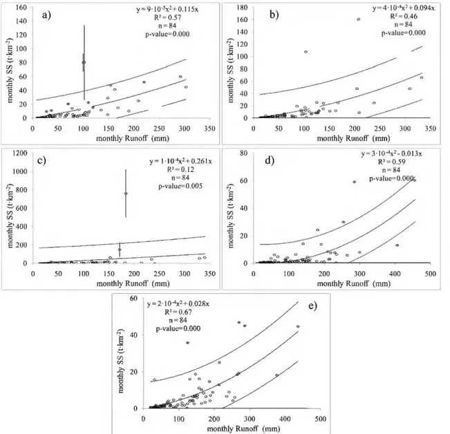
500 500 monthly Runoff (mm)

Figure 7. Regressions and 95% confidence intervals between the monthly specific mean suspended sediment loads (SSLs, in t km-2) and monthly

runoff (in millimetres) for the (a) Deba, (b) Urola, (c) Oria, (d) Urumea and (e) Oiartzun catchments for the period between 2006 and 2013. Standard deviation of the monthly SSL is represented by a vertical line. The regression equation, number of observations (n), determination coefficient (/f) and significanœ lever (p-value) are also shown.

as land-use and catchment geomorphology. ln contrast, to de-tect possible effects on the SS delivery in the analysed catch-ments, the data outside of the 95% interval were considered to be affected by uncommon conditions such as civil engineer-ing works or extraordinary runoff events for points above the confidence interval or sediment retention structures for points below the confidence interval. To estimate the amount of sedi-ment that was delivered due to those conditions, the difference between the line drawn at the 95% confidence interval and the mean of the estimated data was calculated.

ln Oria and Urumea (Figures 7c and 7d), the outlier data are related to the extraordinary runoff event that occurred in November 2011 (Figures 2c, 2d, Sc and Sd). During that month, 250 (± 120)% more SS than that occurring under normal conditions was delivered in Oria and 89 (±3)% more was delivered in Urumea, and in Oiartzun, this event accounted for an extra 29 (± 1 )%. ln Oiartzun, 80 (±2)% and 42 (± 1 )% more SS was transported in September 2011 and November 2009, respectively, likely due to the high discharge amounts observed there for the runoff events of 3 September 2011 and 10 November 2009 (Figure 2e). Finally, in Deba, the outliers accounted for 106 (±34)% and 105 (± 138)% more sediment than normal conditions. ln general, there are few points that are not located inside the 95% confidence interval, and most of them are related to runoff events in which high discharge amounts were observed. Therefore, it can be concluded that in the studied catchments, interannual SS delivery is not contralled by temporally and spatially isolated human impacts, but that more general characteristics of the catchment, such as geomorphology, land-use, general land management, are the drivers of SS availability and, consequently, of SSY.

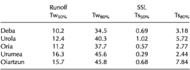
The daily contribution of the runoff and SSL to the total were also calculated. Table IV lists indices of the temporal variability of the discharge and sediment for the five catchments. The results show that a large proportion of the total observed runoff and SS were transported within a short period. The temporal variability in the runoff was not significantly different between the catchments, with 50% of annual water volume exported over 10-16% (1-2 months) of the year (Tw50

o;J

and 80% exported over 35--45% (4--5.5 months) of the year (Tw80%), depending on the catchment. These data demonstrate the high variability of water height in these catchments and how little the catchments are regulated because high values of Tw50% (>30%) are typically observed in highly regulated or lake-influenced rivers (Meybeck

et al.,

2003).

The duration for the SSL was much shorter than that for the water flow. Half of the SSL (Ts50%) was delivered between 0.3% (one day) and 1% (3--4days) of the time, and 80% of the sediment was exported between 2.5% (nine days) and 8% (< 30 days) of the time. Similar data were obtained by Zabaleta and Antiguedad (2012) for three small headwater catchments

Table IV. Temporal variability indices for the runoff (mm) and SS Joad (t) for the five catchments studied. Tw50% and Tw80% are the percentages of time required to deliver 50% and 80% of the annual water volume, respectively. Ts50% and Ts80% are the percentages of time required to deliver 50% and 80% of the annual SS Joad, respectively

Run off SSL

Twso% Twso% Tsso% Tsso%

Deba 10.2 34.5 0.69 3.18

Urola 12.4 40.3 1.02 5.72

Oria 11.2 37.7 0.57 2.77

Urumea 16.3 45.6 0.29 2.44

Oiartzun 15.7 45.8 0.68 7.84

(3.8, 4.8 and 48 km2) in the same area. This contradicts the findings of some authors who show that, sometimes, small events, over long periods, are more responsible than large events for sediment export (Ferro and Porto, 2012). Following the characterization of the duration patterns reported by Meybeck

et al.

(2003), these patterns suggest that the studied catchments show very short sediment flux durations due to small catchment size and scarcity of areas where sediment could be temporally retained (i.e. floodplains). These results are consistent with the relatively high SDR obtained (Table Ill). However, regarding their relationship with catchment area some contradictions can be found since a higher SDR (59%) was estimated for the largest catchments (Oria, 796.5 km2) than for the smallest ones (16%, Oiartzun, 56.6 km2), from which one could conclude that higher amounts of sediment are being deposited in smaller catchments. The contradiction found cou Id be related to the relatively short period of time involved in SSY estimates (seven years). Nevertheless, the catchments with lower SDRs are those with higher RUSLE estimates as well as the steepest slopes and thinner soils. The steepness of those catchments could be related to an overestimation of erasion rates using RUSLE. ln any case, the validity of the RUSLE equa-tion in an enviranment such as that examined in this study can, at least, be discussed.

The duration pattern is also slightly different for SS transport (for some days) and water flow (for some months). lndeed, the Urumea catchment had a higher flow duration (Tw50% = 16.3% of the time) but lower SSL duration (Ts50% = 0.29% of the time). Conversely, Urola, with a similar catchment area, had a lower flow duration (Twso%= 12.4% of the time) but higher SSL du ration (Tsso% = 1.02% of the time). The differ-ences may be related to sediment availability. ln those catch-ments where SS transport is limited by its availability, the du ration for SS would be lower than in those catchments where the availability of SS was notas limited.

These results support the idea that hydroclimatic variables are not the main factors that contrai the spatial variability of the delivery of SS in this area; there must be other, distinct enviranmental parameters that affect SS availability. Various

studies have indicated that factors including

topography/morphology (Pinet and Souriau, 1988; Milliman and Syvitski, 1992; Ludwig and Probst 1996; Montgomery and Brandon, 2002), lithology (Probst and Amiotte-Suchet, 1992; Ludwig and Prabst, 1998; Nadal-Romero

et al.,

2011 ), land-use (Walling, 2006; Lana-Renault

et al.,

2010) and human activities (Olarieta et al., 1999; Siakeu et al., 2004; Evans et al.,

2006) may significantly affect SSY and its variability.

Environmental controls on SS delivery

To explore which factors contrai SS availability in the studied catchments and, consequently, SS delivery to the Bay of Biscay, Spearman correlation coefficients were calculated for ail of the possible variable pairs shown in Table 1 (Table V). Many studies that have examined global SSYs have shown that hydroclimatic variables largely explain the amount of regional variations in SSY. However, contrary to what could be expected, in this area a negative relationship, although statistically not significant, ex-ists between annual precipitation and SSY or SSL and between runoff and SSY or SSL. Taking into consideration the high vari-ability in the hydroclimatic variables in the region, this fact mainly indicates that precipitation or runoff do not limit SS delivery, and other factors exert stranger contrai on SS delivery (Vanmaercke

et al.,

2011 ). There should therefore be physical characteristics of the catchments that li mit sediment availability and thus contrai SS delivery to the ocean. The amount of SS