Reducing the noise of Micro-Air Vehicles in hover

(1)

an author's https://oatao.univ-toulouse.fr/25214

http://www.imavs.org/papers/2017/65_imav2017_proceedings.pdf

Serré, Ronan and Chapin, Vincent and Moschetta, Jean-Marc and Fournier, Hugo Reducing the noise of Micro-Air Vehicles in hover. (2017) In: International Micro Air Vehicle Conference and Flight Competition (IMAV 2017), 18 September 2017 - 21 September 2017 (Toulouse, France).

(2)

Reducing the noise of Micro–Air Vehicles in hover

R. Serr´e*_{, V. Chapin, J.M. Moschetta and H. Fournier}

ISAE–Supaero, DAEP, 10 avenue Edouard Belin, 31055 Toulouse, France ABSTRACT

Micro–Air Vehicles (MAV) are becoming com-mon devices in a wide range of operations while the optimization of their propulsion system is rarely addressed. On the one hand, an aero-dynamic optimization would have a straightfor-ward effect on the endurance. On the other hand, an aeroacoustic optimization might increase dis-cretion in military operating conditions, reduce noise pollution in civilian, urban environment and allow sound recordings in dual applications. This contribution aims at presenting a complete methodology for the design of silent and still effi-cient rotors for MAV, from aerodynamic predic-tion to aeroacoustic optimizapredic-tion and experimen-tal validation. This approach is suitable for engi-neering purposes. The aerodynamic and acous-tic modeling are described and the optimization procedure is presented. A step–by–step opti-mization is achieved and measured on an experi-mental bench suitable for non–anechoic environ-ment. A discussion on the results is proposed. Key parameters on the blade geometry for the re-duction of rotor noise are provided at the end of the paper.

1 INTRODUCTION

Designing a silent rotor goes through an aeroacoustic optimization, which implies understanding the aerodynamic phenomenon responsible for noise generation. Predicting the noise generated aerodynamically is relatively straightforward once detailled aerodynamic involved in the propulsion system is available through the use of direct noise computation or hybrid prediction. Aeroacoustic optimization in that frame-work is possible [1, 2] but demanding in terms of computa-tional cost hence not realistic in an industrial context. Lower– fidelity tools are then needed. Reduction in the rotor noise has received important attention from the early ages of aeroa-coustics [3]. It has yielded a lot of informations and materials which allowed development of low–fidelity models of suffi-cient accuracy. There are identical phenomena that occur in a helicopter rotor and a MAV rotor but the different noise sources do not contribute to the overall noise in the same amount. Detailed analysis of the aerodynamic characteris-tics has to be specifically dedicated to MAV rotors and low– fidelity models should be re–calibrated or at least carefully

*Email address: [email protected]

selected. For the aerodynamic modeling, a widely spread low–fidelity model is used, based on the Blade Element and Momentum Theory (BEMT) [4]. It is fast, reliable but yields a steady loading on the blades. Acoustic is intrinsically un-steady. Because of the relative motion between the spinning blades and a static observer, acoustic radiation can still be re-trieved from a steady loading but it can only be tonal noise as a consequence of a periodic perturbation. As stated by Sini-baldi and Marino [5], the acoustic spectrum radiated by rotors exhibits also a broadband part. Low–fidelity broadband mod-els are then needed in the optimization process in order to get a better description of the acoustic spectrum. The acoustic modeling is realized in two steps: i) an integral method based on the Ffowcs Williams and Hawkings [6] (FWH) equation gives the tonal noise radiated by the rotor from the steady loading yielded by the BEMT and ii) analytical models es-timate the broadband part of the acoustic spectrum based on the work of Roger and Moreau [7]. The optimization pro-cess is allowed by several evolutionary algorithms as will be discussed in a future work while results presented hereby are yielded by a combination method, that is a systematic evalu-ation of the space of parameters. The blade chord and twist laws are parameterized by B´ezier curves considering control points in 4 sections a long the blade span giving 8 variables. However, to ensure lift at blade tip reaches zero to yield a minimum induced velocity, the twist at the fourth control point is imposed at zero eventually giving 7 variables. In the combination method, each variables may take 5 values giving 57 _{individual evaluations. A multi–objective}

selec-tion is applied to express the pareto front according to lower aerodynamic power and lower overall sound pressure level (OASPL). The optimization of the airfoil sections is carried out in a second step through another optimization process. Airfoil shapes are determined using CST parametrization [8] with 12 coefficients. The optimization objective is to maxi-mize the lift-to-drag ratio through NSGA–II evolutionary al-gorithm with a population of about 100 individuals. The final evaluation is achieved after 55 generations.

2 AERODYNAMIC MODELING

Through a BEMT approach as described by Winarto [4], local distributions of lift and drag and global thrust and torque are retrieved from local lift and drag coefficients of the blade element airfoil sections. As a result, knowledge of the aero-dynamic polar of the considered airfoil section is essential to the process. Three strategies may be employed to this end: ex-perimental [9], numerical simulation [10] or numerical mod-eling (such as panel method in potential flow theory [11]).

(3)

The last one is used in the present study for efficiency. Lift and drag coefficients are extracted from Xfoil open–source software by Drela [11], as well as boundary layer data as will be seen in the next section. Figure 1 and figure 2 respectively show lift and drag coefficients prediction by Xfoil compared with experiments from Lyon et al. [9] on an E–387 airfoil sec-tion at Reynolds number Re = 100, 000. Xfoil predicsec-tions exhibit good agreement with experimental data, a severe drag overstimation at high angle of attack notwithstanding.

Fig-Angle of attack (deg.)

-10 0 10 20 30 L if t co effi ci en t Cl -0.5 0 0.5 1 1.5 Experiment Xfoil

Figure 1: Lift coefficient between Xfoil prediction and exper-imental work by Lyon et al. [9] on an E–387 airfoil section at Reynolds number Re = 100, 000.

Angle of attack (deg.)

-10 0 10 20 30 D ra g C o effi ci en t Cd 0 0.1 0.2 0.3 0.4 0.5 Experiment Xfoil

Figure 2: Drag coefficient between Xfoil prediction and ex-perimental work by Lyon et al. [9] on an E–387 airfoil section at Reynolds number Re = 100, 000.

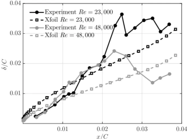
ure 3 depicts boundary layer thickness δ on a NACA 0012 at Reynolds numbers Re = 23, 000 and Re = 48, 000 and a 6° angle of attack, compared with experiments by Kim et al. [12]. The boundary layer behavior experimentally ob-served is dramatically ignored by Xfoil in the medium chord region which shows a monotonic trend. However, the values

does not exhibit too much discrepancy at the trailing–edge re-gion where x/C ∼ 0.04. Boundary layer data needed for the acoustic modeling is extracted from this region as will be seen in the next section. Xfoil is considered reliable and is used to provide input data for the BEMT approach and broadband noise models. x/C 0.01 0.02 0.03 0.04 δ/ C 0.01 0.02 0.03 0.04 Experiment Re = 23, 000 Xfoil Re = 23, 000 Experiment Re = 48, 000 Xfoil Re = 48, 000

Figure 3: Boundary Layer thickness on a NACA 0012 at Reynolds numbers Re = 23, 000 and Re = 48, 000 and a 6° angle of attack between Xfoil prediction and experiments by Kim et al. [12].

3 ACOUSTIC MODELING

The FWH equation is implemented in the time domain as expressed by Casalino [13] in the form known as Formula-tion 1A and applied on the blade surface. Without any fluid volume inside the control surface, the quadrupole term repre-sentative of flow non–linearities is neglected but is believed to be of small contribution in this low–Reynolds, low–Mach number regime, typically encountered in MAV rotors [5]. The FWH equation then only resumes to thickness noise and load-ing noise through surface integrations. The main input pa-rameters are the velocity of the blade element that influence the thickness noise and the force distributions that act on the loading noise. In that steady loading framework, the latter is found to be relatively small without significantly contribut-ing to the overall noise. In this study, the thickness noise is found to be dominant independently of the observer’s loca-tion. In addition, two sources of broadband noise are con-sidered, based on reference [7]: the scattering of boundary layer waves by the trailing–edge and the ingestion of turbu-lence at the leading–edge. Roger and Moreau [7] mention a third source of broadband noise, that is the shedding of vor-tical eddies in the wake. This source will be considered in a future work. The main input for the trailing–edge noise model are a wall–pressure spectrum model as proposed by Kim and George [14] for instance and a spanwise correlation length as modeled by Corcco [15]. The boundary layer data

(4)

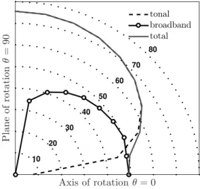
near the trailing–edge is crucial. This source of broadband noise does not appear to contribute significantly to the over-all noise. However, its relevance is supported by the authors to prevent optimization cases where it might overcome tonal noise, as discussed by Pagliaroli et al. [16], especially if tonal noise is to be reduced. For the turbulence ingestion noise model, information on impinging turbulence is required. The driving parameters are the cross–correlated upwash velocity fluctuations spectrum such as von K´arm´an model [17], the mean intensity of the chordwise velocity fluctuations and the Taylor micro–scale as the turbulence length scale. The lat-ter is estimated by the numerical tool from the wake width created at trailing–edge [18] that is believed to impinge the following blade’s leading–edge [19]. It is believed by the au-thors to be the dominant source of noise in MAV rotors [19]. These broadband noise models estimate the noise in the form of a power spectral density, generated in the trailing–edge and the leading–edge regions from boundary layer data and tur-bulence statistics through a correlation function modified by a Doppler shift imposed by the relative motion between the source and the observer. For the optimization process, only one observer is considered, located 45° above the plane of rotation, 1 m away from the center of rotation. Because the noise models exhibit a symetrical behavior with respect to the plane of rotation, selecting an observer position 45° above or below that plane of rotation leads to the same conclusions. This location has been chosen as compromise following

ob-Axis of rotation θ = 0 P la n e o f r o t a t io n θ = 9 0 10 20 30 40 50 60 70 80 tonal broadband total

Figure 4: Illustration of the directivity from the noise predic-tion models. The levels are in dB.

servation of figure 4 which depicts the overall sound pres-sure level (OASPL) in dB for the tonal noise, the broadband trailing–edge noise and the total noise of a representative ro-tor blade, for elevation angles between θ = 0° (on the axis of rotation) and θ = 90° (on the plane of rotation). Formulation

1A of the FWH equation gives a singular value on the axis of rotation while the trailing–edge noise model has its singu-larity on the plane of rotation. These two observation angles should then be avoided.

4 METHODOLOGY

Relatively low optimization studies on low–Reynolds ro-tors have been published with regards of the general interest in MAVs and the recent observation that noise from MAVs is generally considered as annoying [20]. Gur and Rosen have proposed a rotor optimization based on aerodynamic ef-ficiency [21]. With aeroacoustic objectives, the reader might refers to Pagano et al. [1] and Pednekar et al. [2] whose op-timization is based on high fidelity numerical simulations. Studies from Wisniewsky et al. [22] and Zawodny et al. [23] used low fidelity models but at relatively high Reynolds num-bers and based on empirical data for symetrical airfoil sec-tions and for that reason theses studies are believed by the au-thors to lack generality. To demonstrate the feasability of the optimization methodology and to identify the key parameters of the blade geometry allowing noise reduction, a step–by– step optimization of a two–bladed rotor is carried for succes-sive blade geometries:

1. constant chord and constant twist with a NACA 0012 airfoil section

2. same constant chord and optimized twist with a NACA 0012 airfoil section

3. optimized chord and twist with a NACA 0012 airfoil section

4. previous blade geometry with optimized airfoil sec-tions

The successive optimizations occur at iso–thrust, that is to say, the rotational speed is adapted so that the optimized ro-tors deliver the same thrust, set at 2 N. The optimized ge-ometry is selected to minimize both the aerodynamic power and the OASPL at one specific observer position. At the time the optimizations were carried out, only the trailing– edge noise model was active. The blade geometries are then builded using SLA technolgy on a FormLabs 3D–printer with a 50 µm vertical resolution for experimental purposes. The maximum radius is the same for all the rotors and is set at

R = 0.0875m, imposed by the printing volume allowed by

the 3D–printer.

5 NUMERICALRESULTS

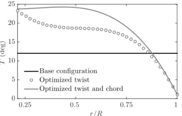
The successive configurations show an increased twist, along with an increase of the chord for the third optimiza-tion. For that optimized rotor, the chord monotonically de-creases with the span (figure 5), while the twist is high at the hub, slightly increases at mid–span before reaching a mini-mal value at the tip (figure 6). The span direction and the

(5)

chord are normalized by maximum radius of the rotors. A CAD representation of the four rotors is depicted in figure 7. The fourth rotor is obtained from the third one (with

op-r/R 0.25 0.5 0.75 1 T (d eg ) 0 5 10 15 20 25 Base configuration Optimized twist

Optimized twist and chord

Figure 5: Twist distribution laws of the successive rotors.

r/R 0.25 0.5 0.75 1 c/ R 0.1 0.2 0.3 0.4 0.5 Base configuration Optimized twist

Optimized twist and chord

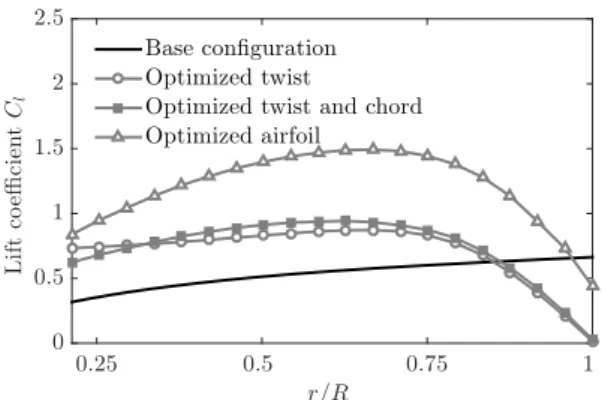
Figure 6: Chord distribution laws of the successive rotors. timized chord and twist) with additional airfoil section opti-mization. Three airfoil sections at three radial positions are depicted on figure 8. They were obtained by an optimization process as described in the introduction of the present paper to maximize the lift–to–drag ratio on an average in angles of attack at the specified radial positions. The optimized airfoil sections are all thinner than the reference one and cambered as can be expected for low–Reynolds number aerodynamics. The airfoil section near the tip region (r/R = 1) exhibits a bump on the suction side, that might indicate an adaptation to separation phenomenon on a specific local Reynolds number. It might be avoided if the airfoil optimization occurs on an average in Reynolds numbers. Figure 9 and 10 show lift and drag coefficients respectively, distributed along the span for the successive blades. The lift coefficient is successively in-creased with a maximum localized around 75% of the blade radius. The drag coefficient is also increased although less intensively with a maximum value localized around 65% of

Figure 7: CAD representation of the four rotors considered in the present study. From left to right: initial rotor (base con-figuration), optimized twist, optimized twist and chord and additional optimized airfoil sections.

r/R = 1.0 (Re = 42, 000) NACA 0012 Optimized airfoil r/R = 0.5 (Re = 82, 000) r/R = 0.1 (Re = 32, 000) 0 1

Figure 8: Optimized airfoil sections for the fourth rotor com-pared with the base configuration (NACA 0012).

the blade radius. The lift coefficient is seen to have been mul-tiplied by three while the drag coefficient has been mulmul-tiplied by two. The gain in aerodynamic efficiency for the succes-sive optimizations yields a diminution of the rotational speed required to deliver the thrust objective set at 2 N (table 1) re-sulting in a diminution of the blade passing frequency (BPF) (table 2). The tendency of the optimizations to move the BPF towards low frequencies has an effect on the noise reduction for low frequencies are less perceived by human ear. During the optimization process, the sole trailing–edge noise model was active. Figure 11 is presented to assess the ability of the optimization tool to reduce overall noise with the trailing– edge noise model. In figure 11, the blade element contri-bution to overall noise is shown for the four configurations. For the base configuration, the blade element contribution in-creases almost linearly toward the tip region according to a Reynolds number effect. The three successive optimizations have a zero twist angle at the tip and it results in a drasti-cally reduced radiated noise near the tip region. The third and fourth optimization cases express a lower radiated noise

(6)

Numerical prediction

Base configuration 9310

Optimized twist 7630

Optimized chord and twist 6010

Optimized airfoil 4880

Experiment

Optimized twist 8400

Table 1: Rotational speeds (in rpm) for a 2 N thrust between numerical prediction and experiment for the four successive rotors.

Optimized twist 255

Experiment

Optimized twist 280

Table 2: Blade passing frequency (BPF, in Hz) for a 2 N thrust between numerical prediction and experiment for the four successive rotors.

for each blade element although its chord and twist distribu-tion laws are higher that the second optimizadistribu-tion case. The airfoil section optimization increases that tendency. To in-vestigate the noise reduction yielded by the optimization tool for the successive rotors, figures 12 and 13 shows the sound power level predicted by the trailing–edge and the turbulence ingestion noise models, respectively. The sound power level is computed according to ISO 3746 : 1995 standard in third octave bands for the successive rotors at a 2 N thrust. The important difference in magnitude between the two numeri-cal models is noteworthy. The numerinumeri-cal tool suggests that turbulence ingestion is a more intense source of noise than trailing–edge noise and can overcome the main tonal compo-nent at the first BPF. From the two noise models, noise reduc-tion is observed for the successive optimizareduc-tions. The main tonal noise component that occurs at the first BPF is reduced at each optimization case, up to 25 dB(A) with the fourth ro-tor as observed in both figures 12 and 13. From the second optimization, the trailing–edge noise is dramatically reduced and the following optimizations increase that tendency (fig-ure 12). The turbulence ingestion noise is also systematically reduced (figure 13). r/R 0.25 0.5 0.75 1 L if t co effi ci en t Cl 0 0.5 1 1.5 2 2.5 Base configuration Optimized twist

Optimized twist and chord Optimized airfoil

Figure 9: Spanwise lift coefficient distribution of the succes-sive rotors for a 2 N thrust. Numerical prediction.

r/R 0.25 0.5 0.75 1 D ra g co effi ci en t Cd 0.01 0.02 0.03 0.04 0.05 0.06 0.07 Base configuration Optimized twist

Figure 10: Spanwise drag coefficient distribution of the suc-cessive rotors for a 2 N thrust. Numerical prediction.

6 EXPERIMENT

The experiment took place in a rectangular room, not acoustically treated, of dimensions (l1× l2× l3) = (14.9×

4.5× 1.8) m3_{. The aerodynamic forces are retrieved from a}

five components balance. The sound power level and the total acoustic power are computed according to ISO 3746 : 1995 standard with five measurement points approximately 1 m around the rotor on Br¨uel & Kjær 1/200 _free–field

micro-phones and a Nexus frequency analyzer with a frequency res-olution of 3.125 Hz. The distance between the source and the microphones approximately represents 5 rotor diameters. Four of the microphones are on a meridian line parallel to the ground and centered on the axis of rotation. The fifth micro-phone is located in the plane of rotation. Figure 14 exhibits thrust measurements and numerical predictions for the four successive configurations and several rotational speeds. Mea-surements and numerical predictions express the same trend, a slight discrepancy observed for the third and fourth opti-mizations notwithstanding. Such a discrepancy is explained with the last two rotors having a significant mass, resulting in an actual thrust different for the prediction. The mass of the

(7)

r/R 0.25 0.5 0.75 1 O A S P L (d B ) 0 10 20 30 40 50 60 Base configuration Optimized twist

Figure 11: Spanwise blade element contribution to the over-all sound pressure level (OASPL) for a 2 N thrust for the suc-cessive rotors. Numerical prediction from the trailing–edge noise model.

Third Octave Centered Frequency Band (Hz) 125 200 315 500 800 1250 2000 3150 5000 S o u n d P ow er L ev el d B (A ) 0 20 40 60 80 100 120 Base configuration Optimized twist

Figure 12: Sound power level of the acoustic spectrum of the successive rotors for a 2 N thrust. Numerical prediction from the trailing–edge noise model.

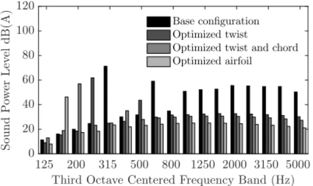
first two rotors is 8.1 g, while the mass of the last two rotors is 21.0 g representing 4% and 10% of the thrust objective, respectively. Figure 15 shows the sound power level com-puted according to ISO 3746 : 1995 standard in third octave bands for the successive rotors at a 2 N thrust from exper-iment. It can be directly compared with figures 12 and 13. Noise reduction is effectively observed, although less than the noise reduction observed from numerical predictions (fig-ures 12 and 13). In the experiment, the main tonal compo-nent at the first BPF is reduced by a maximum of 15 dB(A) between the base configuration and the fourth rotor, where the numerical tool predicted a noise reduction by 25 dB(A). Noise reduction occurs in every frequency bands whereas the numerical tool predicted higher low frequencies. Compar-ing figure 15 with figures 12 and 13 suggests evidences that turbulence ingestion noise might be the dominant source of broadband noise. A slight overestimation by the numerical tool at highest frequencies is however to be expected.

Third Octave Centered Frequency Band (Hz) 125 200 315 500 800 1250 2000 3150 5000 S o u n d P ow er L ev el d B (A ) 0 20 40 60 80 100 120 Base configuration Optimized twist Optimized twist and chord Optimized airfoil

Figure 13: Sound power level of the acoustic spectrum of the successive rotors for a 2 N thrust. Numerical prediction from the turbulence ingestion noise model.

Rotational speed (rpm) 2000 3000 4000 5000 6000 7000 8000 T h ru st (N ) 0 1 2 3 4 5 6 Base configuration (N) Optimized twist (N) Optimized twist and chord (N) Optimized airfoil (N) Base configuration (E) Optimized twist (E) Optimized twist and chord (E) Optimized airfoil (E)

Figure 14: Thrust evolution with rotational speed of the suc-cessive rotors from numerical prediction and experiment. The horizontal dash line (red) indicates thrust objective at 2 N. N: numerical predictions. E: experiment.

7 RESULTS AND DISCUSSION

It appears more clearly on figure 16 why turbulence in-gestion noise is believed to be the dominant source of noise in MAV rotors. Figure 16 shows the sound power level com-puted according to ISO 3746 : 1995 standard in third oc-tave bands for the final optimized rotor at a 2 N thrust from measurements and numerical predictions (trailing–edge and turbulence ingestion noise models). The trailing–edge noise model predicts sound power levels than do not reach the sound power levels observed in the experiment. On the con-trary, the turbulence ingestion noise model seems able to pre-dict accurately the broadband components of the sound power spectrum. The experimental data is slightly higher than the numerical predictions but it is reminded that the rotational speed needed to reach the thrust objective is higher in the ex-periment than in the numerical tool. The exceeding sound power levels seen from the experiments are sub–harmonics

(8)

Third Octave Centered Frequency Band (Hz) 125 200 315 500 800 1250 2000 3150 5000 S o u n d P ow er L ev el 0 20 40 60 80 _{Optimized airfoil}

Figure 15: Sound power level of the acoustic spectrum of the successive rotors for a 2 N thrust. Experiment.

Third Octave Centered Frequency Band (Hz) 125 200 315 500 800 1250 2000 3150 5000 S o u n d P ow er L ev el d B (A ) 0 20 40 60 80 100 120 Experiment

Numerical prediction (trailing–edge) Numerical prediction (turbulence ingestion)

Figure 16: Sound power level of the acoustic spectrum of the final optimized rotor for a 2 N thrust.

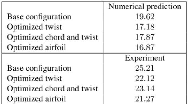
tonal peaks that are not retrieved from the tonal noise model in the numerical tool as a consequence of the steady aero-dynamic input data. These peaks, as well as the main tonal component at the first BPF that are higher in the experiments are a consequence of unsteady loading occuring during the experiment and may more specifically be a consequence of installation effects. The experimental test bench holds the ro-tor in such a way that its axis of rotation is parallel to the ground. As a consequence, a stand that includes the aero-dynamic balance is mounted vertically, behind the rotor and it might yield additional noise radiation at the BPFs. More-over, the motor radiates its own noise that has not been iden-tified by the authors. As long as these additional sources of noise are not isolated, a straightforward identification of the sources of noise in the rotor can not be carried out from a typical narrow–band frequency spectrum. Eventually, the following tables exhibit comparison between numerical pre-dictions and experiment on the aerodynamic power (table 3) and on the total acoustic power (table 4). The aerodynamic power is underestimated by the numerical tool by almost 6 W but the power reduction is higher in the experiment (table 3). The total acoustic power is underestimated by the

numeri-ration notwithstanding. As a result, the reduction in the to-tal acoustic power is amplified by the numerical (table 4).

Base configuration 19.62

Optimized twist 17.18

Optimized chord and twist 17.87

Optimized airfoil 16.87

Experiment

Base configuration 25.21

Optimized twist 22.12

Optimized chord and twist 23.14

Optimized airfoil 21.27

Table 3: Aerodynamic power in Watts for the four successive rotors for a 2 N thrust.

NTE NTI EXP

Base configuration 72.0 85.0 83.3

Optimized twist 61.9 81.2 81.3

Optimized chord and twist 57.0 77.1 76.6

Optimized airfoil 46.6 71.1 74.5

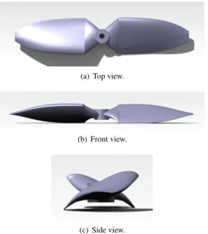
Table 4: Total acoustic power in dB(A)for the four successive rotors for a 2 N thrust. NTE: numerical prediction from the trailing–edge noise model. NTI: numerical prediction from the turbulence ingestion noise model. EXP: experiment. The general trend of the optimization process as shown in ta-bles 3 and 4 is promising: a reduction by 9 dB(A) in the total acoustic power reduction is experimentally observed together with a reduction by 4 W in the aerodynamic power and that is achieved at a minimum cost thank to the numerical tool. Closer views of the most efficient rotor of the successive con-figurations are shown in figure 17.

8 CONCLUSION

The successive optimizations presented in this study al-low to draw the folal-lowing conclusions: adapting the twist increases the lift coefficient but more severely increases the drag coefficient as well. Adapting both chord and twist does not affect the lift coefficient but decreases significantly the drag coefficient. Adapting the airfoil section increases again the lift coefficient but with a slight increase in drag coeffi-cient. On the acoustic reduction, the main effect of the opti-mizations is to provide higher aerodynamic efficiency that al-low to decrease the rotational speed which has two effects: i) to lower the main frequency of the tonal noise and ii) to weaken the intensity of the turbulent eddies that create tur-bulence ingestion noise. The effect is a direct reduction in

(9)

(a) Top view.

(b) Front view.

(c) Side view.

Figure 17: CAD representation of the optimized rotor. It ra-diates 10 dB(A) less and consummes 4 W less for the same thrust production.

the radiated acoustic energy. The turbulence ingestion is con-sidered the dominant source of broadband noise in MAV ro-tors. As it is generated in the vicinity of the leading–edge, a biomimetic leading–edge design [24] might help reaching higher levels of noise reduction. Other factors that might also contribute to reduce the noise in MAVs include blade ra-dius and number of blades: increasing the blade rara-dius would increase the aerodynamic efficiency and lower the rotational speed while an odd number of blades is perceived as less an-noying as mentionned in a recent psychoacoustic study [20]. This study has contributed to the validation and the demon-stration of the efficiency of the low–cost methodology pre-sented in this paper for reducing rotor noise and increas-ing endurance of Micro–Air Vehicles. The numerical tool and the experimental protocole described in the present pa-per are suitable for engineering purposes. Reducing the noise from MAVs in hover can then be achieved without expensive means.

ACKNOWLEDGEMENTS

This study is support by Direction G´en´erale de l’Armement (DGA). Authors thank Sylvain Belliot for the rapid prototyping and Marc C. Jacob for helpful discussions.

REFERENCES

[1] A. Pagano, M. Barbarino, D. Casalino, and L. Federico. Tonal and broadband noise calculations for aeroacous-tic optimization of propeller blades in a pusher

configu-ration. In 15th AIAA/CEAS Aeroacoustics Conference, number AIAA-2009-3138, 2009.

[2] S. Pednekar, D. Ramaswamy, and R. Mohan. Helicopter rotor noise optimization. In 5th Asian-Australian Rotor-craft Forum, 2016.

[3] F. Farassat. Theory of noise generation from mov-ing bodies with an application to helicopter rotors. NASA, Technical Report R-451, 1975.

[4] H. Winarto. BEMT algorithm for the prediction of the performance of arbitrary propellers. Melbourne: The Sir lawrence Wackett Centre for Aerospace Design Technology, Royal Melbourne Institute of Technology, 2004.

[5] G. Sinibaldi and L. Marino. Experimental analysis on the noise of propellers for small UAV. Applied Acous-tics, 74:79–88, 2013.

[6] J. E. Ffowcs Williams and D. L. Hawkings. Sound gen-eration by turbulence and surfaces in arbitrary motion. Philosophical Transactions of the Royal Society of Lon-don, 264(1151):321–342, 1969.

[7] M. Roger and S. Moreau. Extensions and limitations of analytical airfoil broadband noise models. International Journal of Aeroacoustics, 9(3):273–305, 2010.

[8] B. R. Kulfan. Universal parametric geometry repre-sentation method. Journal of Aircraft, 45(1):142–158, 2008.

[9] C. A. Lyon, A. P. Broeren, P. Gigu`ere, A. Gopalarath-nam, and M. S. Selig. Summary of low–speed airfoil data volume 3. SoarTech Publications, Virginia Beach, VA, 1998.

[10] J. Morgado, R. Vizinho, M. A. R. Silvestre, and J. C. P´ascoa. XFOIL vs CFD performance predictions for high light low Reynolds number airfoils. Aerospace Sci-ence and Technology, 52:207–214, 2016.

[11] M. Drela and M. B. Giles. Viscous–inviscid analysis of transonic and low Reynolds number airfoils. AIAA Journal, 25(10):1347–1355, 1987.

[12] D. H. Kim, J. H. Yang, J. W. Chang, and J. Chung. Boundary layer and near–wake measurements of NACA

0012 airfoil at low Reynolds numbers. In 47th

AIAA Aerospace Sciences Meeting, number AIAA-2009-1472, 2009.

[13] D. Casalino. An advanced time approach for acoustic analogy predictions. Journal of Sound and Vibration, 261:583–612, 2003.

(10)

[14] Y. N. Kim and A. R. George. Trailing–edge noise from hovering rotors. AIAA Journal, 20(9):1167–1174, 1982. [15] Y. Rozenberg, M. Roger, and S. Moreau. Rotating blade trailing–edge noise : experimental validation of analyti-cal model. AIAA Journal, 48(5):951–962, 2010. [16] T. Pagliaroli, J. M. Moschetta, E. B´enard, and C. Nana.

Noise signature of a MAV rotor in hover. In 49th 3AF in-ternational symposium of applied aerodynamics, 2014. [17] R. K. Amiet. Acoustic radiation from an airfoil in

a turbulent stream. Journal of Sound and Vibration, 41(4):407–420, 1975.

[18] T. Fukano, Y. Kodama, and Y. Senoo. Noise generated by low pressure axial flow fans, I: modeling of the tur-bulent noise. Journal of Sound and Vibration, 50(1):63– 74, 1977.

[19] R. Serré, N. Gourdain, T. Jardin, A. Sabaté López, V. Sujjur Balaramraja, S. Belliot, M. C. Jacob, and J. M. Moschetta. Aerodynamic and acoustic analysis of an optimized low reynolds number rotor. In 17th Inter-national Symposium on Transport Phenomena and Dy-namics of Rotating Machinery, 2017.

[20] N. Kloet, S. Watkins, X. Wang, S. Prudden, R. Cloth-ier, and J. Palmer. Drone on: a preliminary investiga-tion of the acoustic impact of unmanned aircraft sys-tems (UAS). In 24th International Congress on Sound and Vibration, 2017.

[21] O. Gur and A. Rosen. Optimization of propeller based propulsion system. Journal of Aircraft, 46(1):95–106, 2009.

[22] C. F. Wisniewski, A. R. Byerley, W. H. Heiser, K. W. Van Treuren, and W. R. Liller. Designing small pro-pellers for optimum efficiency and low noise footprint. In 33rd AIAA Applied Aerodynamics Conference, num-ber AIAA-2015-2267, 2015.

[23] N. S. Zawodny, D. Douglas Boyd Jr, and C. L. Burley. Acoustic characterization and prediction of representa-tive, small–scale rotary–wing unmanned aircraft system components. In 72nd AHS Annual Forum, 2016. [24] P. Chaitanya, P. Joseph, S. Narayanan, C. Vanderwel,

J. Turner, J. W. Kim, and B. Ganapathisubramani. Per-formance and mechanism of sinusoidal leading edge serrations for the reduction of turbulence–aerofoil inter-action noise. Journal of Fluid Mechanics, 818:435–464, 2017.